Solar Power Forecasting

(1)

SOLAR POWER FORECASTING

A

thesis

submitted

in

fulfilment

of

the

requirements

for

the

degree

of

Doctor

of

Philosophy

in

the

School

of

Computer Science

at

The University of Sydney

Zheng Wang September 2019

(2)

c

Copyright by Zheng Wang 2019

All Rights Reserved

(3)

Abstract

Solar energy is one of the most promising environmentally-friendly energy sources. Its market share is increasing rapidly due to advances in PhotoVoltaic (PV) technologies, which have led to the development of more efficient PV solar panels and the significant reduction of their cost. However, the generated solar energy is influenced by meteo-rological factors such as solar radiation, cloud cover, rainfall and temperature. This variability affects negatively the large scale integration of solar energy into the elec-tricity grid. Accurate forecasting of the power generated by PV systems is therefore needed for the successful integration of solar power into the electricity grid. The ob-jective of this thesis is to explore the possibility of using machine learning methods to accurately predict the generated solar power so that this sustainable energy source can be better utilized. We consider the task of predicting the PV power for the next day at half-hourly intervals.

At first, we explored the potential of instance-based methods and propose two new methods: the data source weighted nearest neighbor DWkNN and the extended Pat-tern Sequence Forecasting (PSF) algorithms. DWkNN is an extension of the standard nearest neighbour algorithm; it uses multiple data sources (historical PV power data, historical weather data and weather forecasts) and considers the importance of these data sources in the final prediction by learning the best weights for them based on pre-vious data. PSF1 and PSF2 are extensions of the standard PSF algorithm which is only applicable to a single data source (historical PV data) to deal with data from multiple related time series. Our evaluation using Australian data showed that the proposed extensions were more accurate than the methods they extend.

Then, we proposed two clustering-based methods for PV power prediction: di-rect and pair patterns. Many recent algorithms create a single prediction model for all weather types. In contrast, we used clustering to partition the days into groups with similar weather characteristics and then created a separate PV power prediction model

(4)

for each group. The direct clustering groups the days based on their weather profiles, while the pair patterns considers the weather type transition between two consecu-tive days. The proposed methods were evaluated and compared with methods without clustering using Australian data. The results showed that clustering-based models out-performed the other models used for comparison.

We also investigated ensemble methods and proposed static and dynamic ensem-bles of neural networks. We proposed three strategies for creating static ensemensem-bles based on random example and feature sampling, as well as four strategies for creat-ing dynamic ensembles by adaptively updatcreat-ing the weights of the ensemble members based on past performance. Our results showed that all static ensembles were more ac-curate than the single prediction models and classical ensembles used for comparison, and that the dynamic ensemble further improved the accuracy. We then explored the use of meta-learning to improve the performance of the dynamic ensembles. Instead of calculating the weights of the ensemble members based on their past performance, meta-learners were trained to predict the performance of the ensemble members for the new day and calculate the weights accordingly. The results showed that the use of meta-learning further improved the accuracy of dynamic ensemble.

The methods proposed in this thesis can be used by PV plant and electricity market operators for decision making, improving the utilisation of the generated PV power, avoiding waste, planning maintenance and reducing costs, and also facilitating the large-scale integration of PV power in the electricity grid.

(5)

(6)

Acknowledgements

I would like to thank all people who have encouraged and supported me to complete this thesis.

I would like to express my sincere gratitude to my supervisor, Associate Professor Irena Koprinska, from the School of Computer Science at the University of Sydney, for her continuous support of my research, which has helped me to successfully grow as a research data scientist. She guided me to explore and clarify my research direction in the beginning of my research work and provided consistent guidance with infinite patience throughout my PhD study. Moreover, I appreciate her kind help and comfort when I suffered from deep sorrows and got lost. Thanks to her consistent help, I finally completed this thesis. I also want to thank Dr Mashud Rana and Dr Ling Luo for their help and technical support. It is my honor to have collaborated with them during my research studies.

I would also like to thank my parents for their endless support and their unreserved love all the time. When I struggled with my research work and almost lost all patience and motivation, it is their love and unlimited encouragement that helped me overcome all the difficulties. I appreciate all the sacrifices they made for me.

I would like to thank the Australian Government for granting me the Postgradu-ate Award, which reduced my financial burden and enabled me to concentrPostgradu-ate on my research work. Special thanks to Associate Professor Xiuying Wang and her research team for their support during my PhD studies.

Finally, I would like to thank my friends Jingcheng Wang, Sheng Hua, Hui Cui, Chaojie Zheng and Yu Zhao for their company, encouragement and kind help with my research work. I can hardly bring this thesis to this successful ending without their support.

(7)

List of Figures

3.1 The DWkNN algorithm . . . 29

3.2 Representing days using historical PV and weather data . . . 31

3.3 Representing days using historical PV data and weather forecast . . . 31

3.4 Representing days using historical weather data and weather forecast . 32 3.5 Representing days using historical PV and weather data, and weather forecast . . . 32

3.6 PV power data from Jan 2015 to Dec 2016 . . . 34

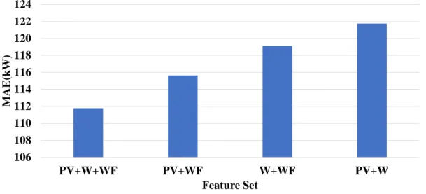
3.7 kNN performance (MAE) using different feature sets . . . 39

3.8 DWkNN performance (MAE) using different feature sets . . . 41

3.9 Comparison between DWkNN andkNN (MAE) . . . 41

3.10 Comparison of all prediction methods (MAE) . . . 43

3.11 Comparision between DWkNN-WF and DWkNN-WF2 . . . 44

3.12 PSF for time series prediction . . . 47

3.13 PSF for daily PV power output prediction . . . 48

3.14 The proposed extension PSF1 . . . 49

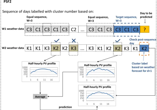
3.15 The proposed extension PSF2 . . . 52

3.16 Two typical daily PV output profiles . . . 59

3.17 Performance of all methods under 10% noise level . . . 60

3.20 Comparison of models under different noise levels . . . 61

4.1 PV power outputs under different weather conditions . . . 65

4.2 Main steps of the proposed clustering based forecasting approaches . 66 4.3 Forecasting using the clustering-basedk-NN . . . 68

4.4 Forecasting using the clustering-based NN . . . 70 xi

(12)

4.5 Forecasting using non-clustering based k-NN . . . 72

4.6 Comparison of clustering based and non-clustering based approaches . 78 4.7 Actual vs predicted data for typical consecutive days from each cluster 79 4.8 The WPP approach . . . 81

4.9 NN prediction model in WPP . . . 83

4.10 Clustering-based methods used for comparison . . . 87

4.11 Comparision of the WPP, clustering-based and non-clustering-based approaches for NN and SVR separately . . . 90

4.12 Performance of all prediction models (MAE) . . . 91

4.13 Comparison of the centroid values . . . 92

5.1 Ensemble EN1 using random example sampling . . . 99

5.2 Ensemble EN2 using random feature sampling . . . 101

5.3 Ensemble EN3 using both random example and feature sampling . . . 103

5.4 Comparison of forecasting methods (MAE) . . . 109

5.5 Comparison of EN3 dynamic ensembles (MAE) . . . 111

5.6 Structure of EN-meta . . . 113

5.7 Training ensemble members . . . 114

5.8 MAE comparison . . . 118

5.9 MAE comparison . . . 120

(13)

List of Tables

3.1 Data sources and feature sets for DWkNN study . . . 34

3.2 Accuracy ofkNN . . . 39

3.3 Accuracy of DWkNN . . . 40

3.4 Statistical Significance Comparison Between kNN and DWkNN for MAE (Wilcoxon Rank Sum Test): -**-Stat. Sign. atp ₆ 0.001, -*-Stat. Sign. atp₆0.05, -x-No Stat. Sign. Difference . . . 42

3.5 Accuracy of the Methods Used for Comparison . . . 43

3.6 Feature Set WF2 . . . 44

3.7 Performance of DWkNN with WF2 . . . 45

3.8 Data sources and feature sets for PSF study . . . 55

3.9 Input and output of the neural models used for comparison . . . 56

3.10 Clustering evaluation results . . . 58

3.11 Bestwfor PSF, PSF1 and PSF2 . . . 58

3.12 Accuracy of all methods . . . 60

4.1 Performance of the clustering based approaches . . . 75

4.2 Performance of the non-cluster based approaches . . . 77

4.3 Performance ofk-NN for each cluster separately, with clustering method 2 . . . 78

4.4 Clustering evaluation results . . . 82

4.5 Accuracy of all methods . . . 91

4.6 Centroids of the two clusters . . . 93

4.7 Detailed information for each pair pattern prediction model for WPP-based NN . . . 93

4.8 Per-cluster comparison of WPP-based NN and Clustering-based NN . 93 5.1 Accuracy of all static methods . . . 108

(14)

5.2 EN3 dynamic ensembles - summary . . . 110

5.3 Accuracy of EN3 dynamic ensembles . . . 111

5.4 Accuracy of EN-meta versions . . . 118

5.5 Accuracy of all models . . . 119

(15)

Chapter 1 Introduction

Solar energy is an important source of renewable energy. It is clean, abundant and easily accessible. Solar energy can be easily collected by using Photo Voltaic (PV) panels, either small-scale roof-top installations or large-scale solar farms. The solar energy can be transformed into electricity and used to supply the electricity in the building or integrated into the electricity grid. In recent years, the PV technology has developed rapidly and is now one of the most promising technologies for producing solar power. The increased efficiency and affordability of PV solar panels has led to the rapid growth of installed PV solar panels around the world, both stand-alone and grid-connected.

Since solar power is environmentally-friendly, many governments are encouraging its use by providing incentives. Due to all these reasons, solar power is expected to contribute significantly to the future global energy supply. For example, it is predicted that the next four years would witness a triple increase in the capacity of the installed PV power systems worldwide, reaching 540GW [1], and that by 2050, about 30% of Australian energy supply will come from PV systems [2].

Even though solar energy has many advantages compared to other traditional en-ergy sources such as coal and natural gas, the produced PV power output is highly variable as it depends on the solar irradiance and other meteorological factors such as solar angle, solar hours, cloud cover, rainfall and temperature. Solar energy is also an intermittent energy source as it is only available during the day time. This variability and intermittence of solar power makes its large-scale integration into the power grid challenging. Unexpected changes in the solar power often happen, negatively affecting

(16)

CHAPTER 1. INTRODUCTION 2

the grid balance and increasing the operational costs. To minimize the possible nega-tive consequences and ensure a larger penetration of PV power in to the energy mix, there is a need for accurate forecasting of the electricity generated by PV systems.

The solar power forecasting methods can be divided into two groups: indirect and direct. The indirect methods firstly predict the solar irradiance and then convert this prediction into solar power output based on the characteristics of the PV plant and other domain knowledge. Technologies such as NWP and satellite image processing are used together to analyze complex meteorological data such as cloud cover move-ment and solar angle changes in order to predict the solar irradiance and make the final prediction [3, 4, 5, 6]. The accuracy of indirect models to a large extent depends on the accuracy of individual components and the availability of weather information. How-ever, the meteorological information required for making accurate indirect forecasts is not always available for the the location of the PV plants. The application of indirect methods also heavily relies on domain knowledge of power engineering. These factors limit the applicability of the indirect methods.

In contrast, the direct group of methods directly predict the output of the PV power systems, without the need to firstly predict the solar irradiance. The main data source is the previous PV power data which is readily available, and the additional data sources include historical weather data and weather forecasts for the new days. This weather information is less complex and easily available for the location of the PV plant than the information required by the indirect methods. Also, the additional data sources can be used to improve the accuracy compared to only using the historical PV power data, but they are no longer indispensable. This enables the wider application of di-rect approaches, compared to the didi-rect ones. The didi-rect approaches can be further divided into two groups, namely statistical and machine learning methods. The former are based on statistical models such as Autoregressive Moving Average (ARMA), Au-toregressive Integrated Moving Average (ARIMA) and Exponential Smoothing (ES) [7, 8, 9, 10, 11]. The latter group applies machine learning algorithms such as Neural Networks(NN)[12, 13, 14], Support Vector Regression (SVR)[15], k Nearest Neigh-bors (k-NN) [16, 7].

This thesis is concerned with developing methods for predicting the power output of solar PV systems. In particular, we focus on directly and simultaneously predict-ing the 24h-ahead solar power output at 30-min intervals. This forecastpredict-ing horizon is frequently used and allows sufficient time for the PV plant and electricity market

(17)

operators to evaluate the situation and make decisions. All case studies in this thesis consider this prediction task. We utilise different data sources, e.g. historical PV power data, historical weather data and weather forecasts. The specific data sources used in different case studies are described in the relevant chapters. The aim of this thesis is to investigate the performance of existing state-of-the-art machine learning methods for solar power forecasting and develop novel methods with improved performance.

1.1 Main Contributions

This thesis focuses on using machine learning approaches to directly and simultane-ously predict the PV power output for the next day at 30-min intervals. We analyze the limitations of the state-of-the-art methods in this area and and propose new methods to address these limitations and improve the accuracy. The main contributions of this thesis can be summarized as follows:

1. Instance-based methods. We propose two new instance-based methods for so-lar power forecasting, namely DWkNN and extended PSF. DWkNN is an exten-sion of k-NN, which considers the importance of different data sources (histori-cal PV power data, histori(histori-cal weather data and weather forecasts) and learns the best weights for them based on previous data. PSF1 and PSF2 are extensions of the standard PSF algorithm which is only applicable to a single data source (historical PV data) to deal with time series from more than one data source. Our evaluation using Australian data showed that the proposed extensions were more accurate than the original methods they extend.

2. Clustering-based methods. We propose two novel clustering-based methods for solar power forecasting that partition the days into groups with similar weather characteristics and then build a separate prediction model for each group. The first method, direct clustering-based method, groups the days into clusters based on their weather profiles and then trains a separate model for each cluster. The second method, weather pair patterns clustering-based method, considers the weather type transition between two consecutive days and then builds a separate prediction model for each type of cluster transition. We evaluated the perfor-mance of the two clustering-based methods and compared them with methods

(18)

without clustering. The results showed that the clustering was beneficial for so-lar power forecasting, resulting in higher accuracy.

3. Ensemble methods. In addition to building single prediction models, we also investigated ensembles of prediction models to improve the forecasting accu-racy. In particular, we investigated ensembles of NNs that use only PV power data since weather data may not always be available for the location of the PV plant. We propose three strategies for creating static ensembles based on ran-dom example and feature sampling, and several strategies for creating dynamic ensembles by adaptively weighting the contribution of the ensemble members based on their recent performance. We also proposed another version of the dynamic ensemble called EN-meta which uses meta-learning and predicted per-formance for the new day instead of actual perper-formance on previous days to calculate the weights of the ensemble members. Our evaluation results showed that proposed ensembles outperformed the single models and classical ensem-bles used for comparison. The dynamic ensemensem-bles were more accurate than the static ensembles, with EN-meta being the most accurate prediction model.

1.2 Publications Associated with the Thesis

The following publications are associated with this thesis:

1. Zheng Wang, Irena Koprinska and Mashud Rana (2016). Clustering Based Methods for Solar Power Forecasting, in Proceedings of theInternational Joint Conference on Neural Networks (IJCNN), Vancouver, Canada, July 2016, IEEE press. CORE ranking: A

2. Zheng Wang, Irena Koprinska and Mashud Rana (2017). Solar Power Predic-tion Using Weather Type Pair Patterns, in Proceedings of theInternational Joint Conference on Neural Networks (IJCNN), Anchorage, May 2017, IEEE press. CORE ranking: A

3. Zheng Wang and Irena Koprinska (2017). Solar Power Prediction with Data Source Weighted Nearest Neighbors, in Proceedings of the International Joint Conference on Neural Networks (IJCNN), Anchorage, USA, May 2017, IEEE press. CORE ranking: A

(19)

4. Zheng Wang, Irena Koprinska and Mashud Rana (2017). Solar power fore-casting using pattern sequences, in Proceedings of theInternational Conference on Artificial Neural Networks, ICANN 2017, Alghero, Italy, September 2017, Springer LNCS.CORE ranking: B

5. Zheng Wang, Irena Koprinska, Alicia Troncoso and Francisco Martinez-Alvarez (2018). Static and Dynamic Ensembles of Neural Networks for Solar Power Forecasting, in Proceedings of theInternational Joint Conference on Neural Net-works (IJCNN), Rio de Janeiro, Brazil, July 2018, IEEE press.CORE ranking: A

6. Zheng Wang and Irena Koprinska (2018). Solar Power Forecasting Using Dy-namic and Meta-Learning Ensemble of Neural Networks, in Proceedings of the International Conference on Artificial Neural Networks (ICANN), Rhodes, Greece, October 2018, Springer LNCS.CORE ranking: B

1.3 Thesis Structure

The rest of the thesis is organized as follows:

Chapter 2 provides a comprehensive review of the previous research work on solar power forecasting. Section 2.1 summarizes meteorological models which use NWP and satellite image processing techniques to make indirect predictions for the PV power output. Section 2.2 reviews statistical models using ARMA, ARIMA and ES. Section 2.3 provides an overview of the state-of-the-art machine learning methods used in this area including single models, clustering-based models and ensembles of predic-tion models. Secpredic-tion 2.4 reviews hybrid systems for solar power forecasting.

Chapter 3 investigates instance-based methods for solar power forecasting and proposes two novel method: DWkNN and extended PSF. Section 3.1 introduces the DWkNN model, which extends the standard k-NN method. Section 3.2 proposes two extended PSF models. Both DWkNN and the extended PSF models are evaluated us-ing Australian data in sections 3.1.2 and 3.2.2 respectively. The publications related to this chapter are publication 3 and 4 from Section 1.2.

Chapter 4 is concerned with clustering-based methods for solar power forecasting. Section 4.1 proposes a new approach based on direct clustering, while Section 4.2

(20)

introduces the weather type pair pattern clustering-based methods. The performance of the proposed methods is evaluated and discussed in sections 4.1.2 and 4.2.2 re-spectively. The publications associated with this chapter are publication 1 and 2 from Section 1.2.

Chapter 5 focuses on exploring the potential of ensembles of prediction models for PV power forecasting. Section 5.1 introduces strategies for creating static and dynamic ensembles based on previous performance. Section 5.2 introduces a dynamic ensemble based on predicted performance for the new day which uses meta-learners. The performance of the proposed methods is evaluated and discussed in sections 5.1.3 and 5.2.2 respectively. The publications related to this chapter are publication 5 and 6 from Section 1.2.

(21)

Chapter 2 Literature Review

As described in Chapter 1, our main research task is to employ machine learning meth-ods to make direct forecasts for the PV power output for the next day. The methmeth-ods used for solar power forecasting can be generally classified into four categories:

1. Meteorological models - These methods ate typically indirect. They use Numer-ical Weather Prediction(NWP) techniques and satellite image processing to first forecast the solar radiation intensity and then convert it into PV output data. 2. Statistical models - These methods usually use statistical methods such as

Auto-Regressive Moving Average (ARMA), Auto-Auto-Regressive Intergrated Moving Av-erage (ARIMA) as well as Exponensial Smoothing (ES). These models can be used to make direct forecasts for the PV power outputs, without the need to firstly forecast the solar irradiance.

3. Machine learning models - These methods use machine learning algorithms such ask-NN, Neural Networks (NN), Support Vector Regression (SVR) and Pattern Sequence-based Forecasting (PSF), to directly forecast the PV power output. There are generally two ways to utilize machine learning techniques: by building a single prediction model or grouping several prediction models together to form an ensemble of prediction models.

4. Hybrid models - These methods combine models or different components from the previous three categories. Slightly different from the ensembles which typ-ically combine machine learning models, the hybrid models usually combine

(22)

CHAPTER 2. LITERATURE REVIEW 8

meteorological models with machine learning and statistical models or compo-nents together.

In the next sections (Section 2.1-2.4), we review the related work in these four categories. The limitations of the current methods and the motivation for our work is discussed in Section 2.5.

2.1 Meteorological Models

A traditional way for forecasting the solar irradiance is to construct physical satel-lite model by measuring local and global meteorological data, and then modeling the relationship between solar irradiance and other factors such as temperature, humid-ity, rainfall values, etc. This process typically needs to convert digital counts from the satellite-based radiometers into flux density, which requires appropriate calibration [17].

2.1.1 Numerical Weather Prediction

The NWP models are usually built on numerical integration equations which require domain knowledge to explain the radiation mechanism and the variations in the atmo-sphere.

In [18] Cornaro et al. pointed out that the key advantage of NWP is that it is a deterministic physical model. However, the authors also indicated that the NWP model is limited by the non-linearity of the domain equations as well as the insufficient spatial resolution of the integration grid, from 100km to a few km, which is too wide compared to the PV plant size. In [19, 20, 21], the spatial resolution of NWP models is discussed. NWP models can be classified into global and mesoscale models. Due to the coarse resolutions, NWP models do not allow the detailed mapping of small-scale features. Although the NWP resolution is improved in recent years, the range of resolutions still lies in 16-50 km depending on the models, which undermines the accuracy of forecasting.

In terms of the temporal scales, Lorenz and Heinemann [22] indicated that NWP models are widely used to predict atmospheric states up to 15 days ahead and this shows the limitation of using NWP models for longer-term forecasts. In summary, the

(23)

accuracy of NWP models depends on the availability of meteorological records and NWP models perform better when applied to short-term prediction tasks.

2.1.2 Satellite Image Processing

Another type of meteorological models used to forecast solar power is based on analysing images captured by digital cameras or satellites [23].

Most existing models which use digital cameras were designed to take images of the hemispheric view of the sky and capture the cloud movement. The movement is then vectorised and used to predict the short-term cloud cover, irradiance and solar power. The efficiency of the cloud tracking and detection techniques is significantly influenced by the ways the cameras are set up [24].

Chow et al. [25], proposed a method for intra-hour, sub-kilometer cloud irradiance forcasting using a ground-based sky imager at the University of California, San Diego. They took sky images every 30s and processed the images to determine the sky cover using a clear sky library and sunshine parameters. They generated a two-dimensional cloud map from coordinate-transformed sky cover to estimate cloud shadows at the surface, which is further used to make the forecasts. The accuracy of the forecasts was mainly influenced by two factors: cloud speed and forecast horizon. The results showed that in the 30s forecasts, the forecasting error was reduced to 50%-60% of the error of the persistence models.

Peng et al. [26] developed a short-term solar irradiance estimation for novel 3D cloud detection and tracking system based on multiple sky imagers. They trained a classifier to recognize clouds at a pixel level as well as the output cloud mask. Then, they measured the block-wise base height and the motion of every cloud layer based on the images captured from the multiple sky imagers, ready to be combined together into larger views for solar prediction. Compared with the persistence model, the proposed model achieved a minimum 36% improvement for all irradiance predictions between 1 min and 15 min intervals.

In addition to images captured by digital cameras from the ground, images captured by satelites were also utilized. The use of satellite images is similar to the use of images captured by cameras on the ground. The cloud pattern is captured and deduced from both the visible and infrared images taken by the satellite sensors flying overhead.

(24)

In [27], Marquez et al. developed the Global Horizontal Irradiance (GHI) pre-dictions at temporal horizons of 30, 60, 90 and 120-min using a hybrid technique of satellite image analysis and NNs. The cloud fraction parameters were collected and used as the NN inputs. The proposed method outperformed the persistence model by 5-19% for 1 time-step forecasts and by about 10-25% for multi-step forecasts. Similar findings can also be found in [28].

Aguiar et al. [29] proposed a satellite-derived ground data model using solar radia-tion and total cloud cover forecasted by European Center for Medium-Range Weather Forecasts (ECMWF) to improve the intra-day solar prediction. They used a clear sky index as a solar radiation parameter with statistical models. A NN was trained with ground and exogenous data as inputs such as history GHI, air temperature and ground relative humidity.

The results showed the combination of NN and ECMWF was beneficial, compared to using NN alone. It improved the RMSE with 15.47%-22.17% for the Co-Pozo Izquierdo station and 25.15%-34.09% for the C1-Las Palmas station.

2.2 Statistical Models

Another important group of methods used to predict the PV power output or solar irra-diance includes statistical models such as Autoregressive Moving Average (ARMA), its extension, Autoregressive Integrated Moving Average (ARIMA), and Exponential Smoothing (ES). These statistical models are usually applied to short-term (within a day) solar power forecasting tasks. Compared to the meteorological forecasting mod-els, statistical models can be directly used to forecast the PV power outputs. This reduces the reliance on domain knowledge about power engineering and PV systems.

2.2.1 ARMA and ARIMA

The general procedure of using ARMA for time series forecasting tasks is as follows [30]:

1. The input data is collected. If the data is non-stationary, then a transformation is conducted to make the data stationary.

(25)

2. The model order (p, d, q)is identified, estimated and fitted. If the model is not adequate, the model order is modified until it becomes adequate.

3. The model is used to forecast as per the desired horizon.

Pedro and Coimbra [7] evaluated five forecasting models with non-exogenous in-puts. They compared ARIMA with a persistent model, standard k-NN, standard NN and a NN optimized by Genetic Algorithms (GA-NN) and tested the accuracy of these models using the data for eight months. Even though the results showed that GA-NN outperformed the other methods used for comparison, ARIMA also showed satisfac-tory accuracy.

Agoua et al. [31] constructed a statistical spatio-temporal method to forecast the power output from several minutes ahead up to 6h ahead. They introduced a new sta-tionarization process to overcome the issue of non-stationarity of the time series. The results show that this pre-processing was beneficial, resulting in better performance compared to using the raw data. They also indicated that including meteorological variables such as wind power contributes to the improvement of the spatio-temporal model. Compared with a persistence model, random forest and AR, the proposed model achieved a 20% higher accuracy.

Yang et al. [32] proposed three forecasting methods to predict the next hour solar irradiance values and the cloud cover effects. The proposed three methods take differ-ent types of meteorological data as input. The first method takes in global horizontal irradiance (GHI) values and directly uses it to forecast the GHI values at 1-hour in-tervals through additive seasonal decomposition, followed by an ARIMA model. The second method forecasts disffuse horizontal irradiance (DHI) and direct normal irradi-ance (DNI) separately using additive seasonal decomposition, followed by an ARIMA model. The results of the two forecasts are then combined to predict GHI using an atmospheric model. The third method considers cloud cover effects and uses ARIMA to predict cloud transients. The final forecasts is made by non-linear regression tech-niques which uses GHI at different zenith angles and under different cloud cover con-ditions. Their results showed that the third method outperformed the other two, leading to MRE = 0.39 and 0.27, RMSE = 29.73 and 32.80 for the Miami and Orland test sets respectively. The results showed that the use of cloud cover techniques improves the performance of the forecasting models.

(26)

Yang et al. [33] proposed AR with eXogenous Input based Statistical model (ARX-ST) to improve the accuracy of PV power forecasting models. The model takes local PV data as well as geographically correlated information of solar PV production from other sites as inputs and can be applied to forecasting tasks for multiple horizons. The results showed that the proposed model was the most accurate for 1-h and 2-h ahead forecasting. For 1-h ahead, MAE of the ARX-ST model was 50.79%, 41.8% and 5.15% lower than the persistence, backpropagation NN, and the AR model, respec-tively. For 2-h ahead, the results were 60.2%, 47.27% and 8.09% ,respecrespec-tively.

Li et al. [11] pointed out that the standard ARIMA for solar power forecasting con-siders only the solar power data and fails to take into account the weather information. Hence, they proposed a generalized model, ARIMAX, which allows for exogenous inputs for forecasting power output. The exogeneous inputs of the model are tem-perature, precipitation amount, insolation duration and humidity, which can be easily accessed. They also indicated that the proposed model is more general and flexible for practical use than the standard ARIMA and improves the performance of the lat-ter based on the experiment results. Their results showed a 36.46% improvement in RMSE, showing that weather information can be used to enhance the performance of ARIMA for solar power forecasting.

2.2.2 Exponential Smoothing

Exponential Smoothing (ES) is a very popular and successful statistical method for forecasting energy time series data such as electricity demand and wind power fore-casting [34, 35, 36, 37]. It computes the prediction as a weighed combination of the previous values, where the more recent values are weighed higher than the older. The Holt-Winters ES is an extension of the standard ES for data with seasonality. This method has also been applied for solar power forecasting.

Yang et al. [10] proposed three time series decomposition based models to forecast the hourly global horizontal irradiance (GHI) values. The first model implemented an additive seasonal-trend decomposition as a pre-processing technique before ES was used, which reduces the state space and hence improves the computational efficiency. The second model decomposed the GHI time series into a direct component and a dif-fuse component. Both components were used to make forecasts and their results were combined using the closure equation, forming the final forecasts for GHI. The third

(27)

method considered also the cloud cover index and applied ES to the cloud cover time series to obtain the cloud cover forecasts. Then, the GHI was forecast through poly-nomial regressions. The results showed that all models outperformed the persistence models.

Dong et al. [9] proposed a Exponential Smoothing State Space (ESSS) model to forecast high-resolution solar irradiance time series. They first built a Fourier trend model to stationarize the irradiance data. This was compared with other state-of-the-arts trend methods using residual analysis and Kwiatkowski-Phillips-Schmidt-Shin (KPSS) stationarity test. Then an ESSS model was implemented to forecast the station-ary residual series of the testing data. They compared the performance with ARIMA, linear exponential smoothing, simple exponential smoothing and random walk mod-els.Their results showed that ESSS generally outperformed the methods used for com-parison.

2.3 Machine Learning Models

The third group of models used for solar power forecasting are based on machine learning and artificial intelligence technique. Most of the state-of-the-arts forecasting models use Neural Networks (NNs), k-Nearest Neighbors (k-NN) and Support Vec-tor Machines (SVM). These models are data-driven and do not require strong domain knowledge of power engineering as required by the meteorological models. Machine learning forecasting models can be used for directly forecasting the PV power, with-out the need to first forecast the solar irradiance and then convert it to power with-output. Another benefit of this group of methods is the flexible forecasting horizon. Most of the meteorological and statistical models introduced in Section 2.1 and Section 2.2 are suitable for short-term or very short-term forecasts, which are usually intra-day fore-casts [38,?, 10, 33], while the forecasting horizon of the machine models can be more flexible, ranging from intra-hours forecasts[39, 40] to next day forecasts [41, 42].

2.3.1 k-NN

k-NN is a popular instance-based method, that has been successfully used for solar power prediction tasks [43, 44, 45].

(28)

Pedro and Coimbra [7] implemented a k-NN model and showed that it outper-formed the persistence model used for comparison. In [16] they also proposed a new

k-NN based methodology to forecast intra-hour GHI and DNI, as well as the corre-sponding uncertainty prediction intervals. The forecasting horizon ranged from 5 min up to 30 min, and the parameters were determined based on an optimization algorithm. The results showed that the proposed model achieved 10% - 25% improvement over the persistence model. The authors also indicated that including sky images in the optimization can lead to a small improvement of about 5%. In [46], they studied the influence of different types of climates into the forecasting perforamnce and proposed

k-NN and NN based models to forecast the global irradiance. The two models were op-timized by using feature extraction methods and the results showed that the proposed models significantly improved the persistence models.

In [47] Chu et al. extended a k-NN model using NN-optimized re-forecasting method. This model was evaluated using the data from a 48MW PV plant and their results showed that the reforecasting method could significantly improve the perfor-mance ofk-NN for time horizons of 5, 10 and 15 min.

Chu and Coimbra [48] proposed k-NN ensemble models using lagged irradiance and image data to generate probability density function forecasts for intra-hour Di-rect Normal Irradiance (DNI). The model took diffuse irradiance measurements and cloud cover information as exogenous feature inputs and was evaluated using data from different locations (continental, coastal and island) by metrics such as Prediction Interval Coverage Probability (PICP), Prediction Interval Normalized Averaged Width (PINAW) and other standard error metrics. As baselines they implemented a persis-tence ensemble probabilistic forecasting model and a Gaussian probabilistic forecast-ing model. Their results showed that the proposedk-NN ensembles outperformed both reference models in terms of all evaluation metrics for all locations when the forecast-ing horizon was longer than 5 mins.

In [49] Chen et al. proposed a methodology to forecast hourly GSI values. More specifically, they trained ak-NN model to preprocess the data prior to training a NN to forecast the 1 hour ahead GSI value for the target PV station. The k-NN model uses meteorological data from 8 adjacent PV stations and generates the inputs for the NN model, which is used to make the forecasts. The results showed that the hybrid model achieved Mean Absolute Bias Error (MABE) of 42 W/m2 and RMSE of 242 W/m2.

(29)

method to predicting energy-related time series. PSF first clusters the historical data into several groups and labels the days with their cluster label. The days prior to the target day form a pattern sequence of cluster labels. PSF then searches the historical data for nearest neighbours of these pattern sequences, and uses the days immediately after the neighbor sequences to compute the forecast for the new days by taking the average of their values. The results showed that PSF was successful and efficient method for making forecasts.

2.3.2 NNs

NNs are the more frequently used methods for solar power forecasting tasks [13, 51, 52, 53]. NNs can be used to solve complex non-linear problems but they require careful parameter selection, including NN structure and training algorithm [54, 55].

Pedro and Coimbra [7] compared k-NN, NN, ARIMA and a persistence model and showed that NN can provide more accurate forecasts for solar power data. They also indicated that the NN can be optimized by Genetic Algorithms, forming GA-NN, which further improves the performance of NN. Izgi et al. [12] proposed an NN model to predict the solar power output of a 750W solar PV panel and compared different forecasting horizons. Their results showed that the best forecasts for short-term and middle-term forecasting horizons were for 5 min and 35 min respectively in April, and for 3 min and 40 min respectively in August.

Chen et al. [56] proposed a forecasting model based on fuzzy logic and NN. It takes as an imput the historical hourly solar irradiation, sky conditions and average hourly temperature, and predicts the solar irradiation values for the next month. Fuzzy logic was used to classify temperature and sky conditions before using them in the NN. An evaluation under different sky conditions was conducted, achieving Mean Absolute Percentage Error (MAPE) ranging from 6.03% to 9.65% for the different cases.

Kardakos et al. [57] compared seasonal ARIMA implemented with solar predic-tion derived from an NWP model and NN with multiple inputs to predict the PV power for both intraday and day-ahead horizons at 1 hour intervals. Their findings showed that the Normalized Root Mean Square Error (NRMSE) of NN model was lower than that of the ARIMA and the persistence model.

Mellit et al. [58] proposed two models based on NNs to forecast solar power gen-erated by 50 Wp Si-Polycrystalline PV modules. The inputs of the models were solar

(30)

irradiance and air temperature. The first NN based model was trained to predict solar PV power in cloudy cases with an average daily solar irradiance less or equal to 400

W m−2/day, and the second model was trained to predict sunny days with the average solar irradiance exceeding 400 W m−2_{. The second NN model showed better} perfor-mance, achieving MBE = 0.94% - 0.98% and RMSE less than 0.2%. The work showed that the performance of NN models may vary under different weather conditions and explored the possibility of training separate classifiers for different weather conditions. The same inputs (solar irradiance and temperature) were used in [59], where Al-monacid et al. proposed a NN model to predict the 1-h ahead PV power output. The model was evaluated using linear regression analysis, which compares the actual val-ues with the forecast valval-ues. The results showed that the proposed model achieved correlation coefficient values close to 1 and RMSE of 3.38%. Similarly, Mellit and Pavan [60] applied NNs to predict the daily solar irradiance at 60-min intervals. In addition to the average daily solar irradiance and temperature, the NN models also take as input information about the day of the month. To predict the PV power out-put, the predicted solar irradiance is multiplied with coefficients based on the PV panel characteristics such as area, efficiency and balance.

Dahmani et al. [61] implemented a NN model to forecast the tilted global solar irradiation derived form the horizontal data gathered from Algeira. The model uses as inputs the horizontal global extra-terrestrial irradiation at 5-min intervals, the dec-lination, zenith angle and azimuth angle. It was was evaluated using data for 2 years showing promising results - the best relative RMSE achieved was 8.82%.

In [62] Teo et al. proposed a NN model based on extreme learning machine algo-rithms to directly forecast the PV power output. They used three data sets to evaluate the performance of the model. They indicated that modifying input variables and in-creasing the size of training samples can significantly improve the performance. This conclusion was also made in [63], where Giorgi et al. compared statistical methods based on multi-regression and Elman NN for 1 to 24h ahead PV power prediction. They pointed out that including all weather parameters as input vector provided the best prediction for PV power. However, in [64], a different conclusion was made by Notton et al. who proposed three NN models, evaluated using the data for 5 years at 10 min intervals from a PV plant in France. The first two NN models used decli-nation, time, zenith angle, 10-min extra-terrestrial horizontal irradiation and 10-min extra-terrestrial horizontal global irradiation as inputs. The third NN model included

(31)

the inclination angle as the additional input. The results showed that the elimination of one of the input variables improved the RMSE and Relative Mean Absolute Error (RMAE) by 9% and 5.5% respectively.

Amrouche et al. [65] utilized NN and spatial modelling methods to provide daily forecasts for the local GHI values. The models takes the weather forecasts provided by the US National Ocean and Atmospheric Administration for four adjacent sites as inputs. They compared the proposed model with geometric and statistical models. The results showed that the NN-based models outperformed the geometric and statistical models used for comparison, achieving the lowest MSE and RSME.

Yona et al. [66] implemented a Recurrent Neural Network (RNN) with fuzzy logic to predict the PV power output for the next day. They used fuzzy model functions to generate insolation forecast data so that the RNN can be trained smoothly. The proposed model was shown to be more accurate than other models used for comparison (a persistence model, a model using fuzzy logic only and a feedforward NN), achieving a best MAE = 0.1327kW.

In [67] Long et al. compared four different methods: NNs, SVR,k-NN and Linear Regression (LR). They studied two groups of inputs: (i) historical PV data only and (ii) a combination of historical PV data and weather information. The evaluation was done on data from a PV plant in Macau, for forecasting horizons up to 3 days ahead. Their results showed that there was no single best performing algorithm for all scenarios, but overall NNs were the most successful.

Azimi et al. [68] proposed a system which combines a clustering algorithm with NNs to predict solar radiation. Firstly, they implemented the transformation based k-means algorithm to classify the time series solar power data into various sets to de-termine irregular patterns and outliers. Then the clustered data was used to train NNs, which were used to make the final predictions. They compared the proposed hybrid system with several statistical models including ES and ARIMA and a persistence model, showing that the proposed hybrid system was the most accurate.

In [13] Chen et al. proposed an approach which firstly uses Self-Organizing Map (SOM) to group data into three clusters using the daily solar irradiance and cloud cover information collected from NWP predictions and then train a Radial Basis Function Neural Network (RBFNN) for each cluster. RBFNN uses as input the average PV power output for the previous day and the weather forecast for the next day average daily temperature, solar irradiance, wind speed and humidity. They achieved MAPE =

(32)

9.45% for sunny days and MAPE= 38.12% for rainy days. A similar idea was followed in [69, 70], where the historical data was partitioned into several groups and then a separate model was trained for each group. The rationale behind this idea is that days with similar weather profiles may have similar PV output characteristics and therefore building separate models for different groups may improve the accuracy.

2.3.3 SVR

Apart from NNs, SVM [71] is another state-of-the-art machine learning algorithm that has been widely used for solar power forecasting. When applied to forecasting tasks, the SVM version for regression tasks, Support Vector Regression (SVR), is used. The SVR prediction models are usually compared with NN prediction models [41, 72, 73, 74].

Shi at al. [69] labelled the days as sunny, foggy, cloudy and rainy based on the weather report from a meteorological station and then trained a separate SVR model for each type of day, that predicts the PV power for the next day. As input they used the PV power output of the nearest day in the training data with the same label, and also the average daily temperature forecast for the next day. The highest accuracy was achieved for sunny days (RMSE = 1.57MW) and the lowest for foggy days (RMSE=2.52MW). In [41] Rana et al. proposed a 2D-interval forecasting model using SVR, which directly forecasts the 2D-interval PV power output from historical solar power and meteorological data. The model was evaluated using Australian PV data for two years. Their results showed that SVR2D provided the most accurate forecasts compared with a number of baselines and other methods used for comparison including NN2D and two persistence models.

Mellit et al. [72] proposed a LS-SVM model to make short-term forecasts for me-teorological time series. As input variables they used the wind speed, wind direction, air temperature, relative humidity, atmospheric pressure and solar irradiance. The SVR model was compared with several NN models (MLP, RBF, RNN and PNN), and the results showed that the LS-SVM model provided more accurate forecasts than the NN models.

Ramli et al. [73] compared SVM and NN for solar irradiance forecasts using data from Jeddah and Qassim in Saudi Aribia. They used direct diffuse and global solar irradiation on the horizontal surface as input data, and evaluated the models in terms of

(33)

RMSE, MRE, correlation coefficient and computation speed. The results showed that the SVM models provided higher accuracy and more robust computation, achieving MRE = 0.33 and 0.51 for the two cities, and faster forecasting speed of 2.15s.

Chen et al. [75], proposed seven SVM models with various inputs, to forecast the daily solar irradiation values. They compared the proposed models with five empirical sunshine-based models (linear, exponential, linear exponential, quadratic and cubic) which use data gathered from three Chinese stations. The SVM models produced 10% lower RMSE compared to the empirical models, showing the promise of SVM models. In [76] Wolff et al. developed SVR models to forecast the PV power data for 15-min and 5-h ahead horizons. The model was developed as an alternative to predic-tion models such as NWP. Their results showed that SVR provided good results for 1-h ahead predictions, while the NWP-based models produced better period forecasts start-ing at 3-h ahead, with the cloud motion vector model bestart-ing the most accurate model among them. They authors suggested that combining the results made by different prediction models could further improve the accuracy.

Ekici [77] proposed a LS-SVM model using RBF kernel to forecast the solar radiation values for the next day. The model used as inputs daily mean and maximum temperature, sunshine duration, and historical solar radiation of the day. The results showed that the proposed model was effective and feasible for the task.

In [74] Mohammadi et al. integrated SVM with a wavelet transform and pro-posed SVM-WT model to forecast horizontal global radiation for an Iranian coastal city. They combined different input parameters such as daily global radiation on a horizontal surface, relative sunshine duration, minimum ambient temperature, relative humidity, water vapour pressure and extra-terrestrial global solar radiation on a hor-izontal surface. The performance was compared with ARMA, NN and Genetic Pro-gramming (GP) models. The results showed that the proposed model outperformed the other models used for comparison.

Olatomiwa et al. [78] proposed the Support Vector Machine Firefly Algorithm (SVM-FFA) to forecast the mean horizontal global solar radiation values. They used sunshine duration, maximum temperature and minimum temperature as inputs. The proposed model was compared with GP and NN models, and the results showed that the proposed model achieved the best RMSE, MAPE, r andR2.

In [79] Yang et al. integrated weather-based hybrid technique with SOM, SVR, Fuzzy Inference and Learning Vector Quantization (LVQ) approaches. The model

(34)

uses SOM and LVQ to categroize historical data based on the PV profile and then trains SVRs using historical solar irradiance, temperature and precipitation probability to make forecasts. The fuzzy inference approach is applied during the forecasting to choose an appropriate trained model based on weather information provided by the Taiwan Central Weather Bureau. The results showed that the proposed method outperformed the NN and SVR approaches.

2.3.4 Ensembles

Instead of training one single model, another idea is to utilize ensembles of prediction models which combine the predictions of several models. The idea behind this is to utilize the diversity among the ensemble members - different ensemble members may be more suitable for different situations. The diversity can be generated by varying the input data used for training, the structure of the prediction models and the types of prediction models used in the ensemble.

In [48] Chu and Coimbra proposedk-NN ensemble model using lagged solar irra-diance and image data to generate probabilistic forecasts for intra-hour Direct Normal Irradiance (DNI). The model took diffuse irradiance and cloud cover information as exogenous feature inputs and was evaluated using data from different locations (con-tinental, coastal and island) using standard error measures and also PICP and PINAW. A persistence ensemble probabilistic model and a Gaussian probabilistic model were used for comparison. The results showed that the proposed k-NN ensemble outper-formed the reference models in terms of all evaluation metrics for all locations when the forecasting horizon was longer than 5-min.

Rana et al. [80] proposed two non-iterative and one iterative ensembles of NNs for forecasting the PV power output of the next day at 30-min intervals. The NN ensemble members differed in the number of hidden nodes and weight initialisation. The individual predictions were combined by taking the predicted median value for each half-hour. The evaluation using Australian data for one year, showed the the iterative ensemble was the most accurate, outperforming an SVR-based method and two persistence baselines.

Another NN-based ensemble method to directly and simultaneously forecast the PV power output for the next day was proposed in [81].

(35)

They first clustered the days based on the weather information and then built a sep-arate NN-based ensemble prediction model for each cluster. The ensemble members were trained to predict the PV power based on the weather data as an input. The eval-uation using Australian data for two years showed that the ensemble method achieved MAE=83.90 kW and MRE=6.88%, outperformed the other models used for compari-son. The use of ensemble was also compared with using a single NN and shown to be beneficial.

Raza et al. [82] proposed an ensemble of NNs to forecast the one-day ahead PV power output. They created 6 ensembles, each combining 15 NNs. The final predic-tion was produced using a Bayesian model averaging. The single NNs belonged to three different NN types: feedforward, Elman and cascade-forward backpropagation networks, had different number of hidden neurons and used difefrent versions of the backpropagation training algorithm. The performance was evaluated using two years of Australian data, and the results showed that the use of ensembles was beneficial.

In [83] Li et al. proposed an ensemble method that builds a separate prediction model at a micro level (for each inverter) and then sums the predictions together to produce the final prediction (at a macro level). The individual ensemble members were trained using PV data only; both NN and SVR prediction models were evaluated as ensemble members. The results showed that the ensemble combining the micro forecasts was more accurate than a single macro level prediction model.

2.4 Hybrid Models

The previous sections discussed the three main groups of solar power forecasting meth-ods - meteorological, statistical and machine learning. There is also some research work on combining methods from these three groups to build hybrid prediction mod-els. We distinguish between ensembles and hybrid models: ensembles combine the predictions of machine learning models only while hybrid models combine the predic-tions of any type of models.

In [84] Bouzerdoum et al. proposed a hybrid model combining seasonal ARIMA and SVM to make short-term PV power forecasts. They evaluated the proposed model using data collected from a 20 kW PV plant and compared the proposed model with single seasonal ARIMA and SVM based models. The results showed that the proposed

(36)

hybrid model outperformed the single models.

Wu et al. [85] implemented a hybrid system which integrated NN, SVM, ARIMA and ANFIS using GA. They collected historical solar power, solar irradiance and tem-perature data, and forecasted the solar power data for three PV plants. Their results showed that the proposed hybrid system was more accurate than the single prediction models which comprised the hybrid system, achieving NRMSE = 5.64%, 3.43% and 6.57% for the three sites respectively.

Dong et al. [86] combined satellite image analysis, ES state space and NN methods in a hybrid system. The satellite image technique was primarily used to detect the cloud movements, while ES was utilized to forecast the cloud cover index. Then a NN was trained using the predicted cloud cover index values to forecast the solar irradiance. The results showed that the proposed hybrid model was more accurate than ARIMA, linear ES, simple ES and random walk.

In [47] Chu et al. proposed a re-forecasting method to forecast the intra-hour power output of a PV plant. The first step of the method was to train baseline models, includ-ing a physical deterministic model based on cloud trackinclud-ing, ARMA and ak-NN model. Then, a NN was employed to optimize the performance of the baseline models. The results showed that the proposed method was effective, significantly improving the performance of the baseline methods for time horizons of 5, 10, and 15 min.

Dolara et al. [87] proposed a hybrid system, called Physical Hybridized Artificial Neural Network (PHANN), that combines NN with an analytical physical model - the Clear Sky solar Radiation Model (CSRM). CSRM was used to determine the time span between the sunrise and the sunset of each day, while the NN was trained to make 24-72 h ahead forecasts of PV power based on the output of the CSRM model. The results showed that PHANN outperformed the NN model without the CSRM components. A similar PHANN model was also proposed in [88] and shown to achieve most accurate results during sunny days compared to weather day types.

In [89] Filipe et al. combined statistical and meteorological methods and proposed a hybrid system to forecast the 48 h ahead solar power output of a PV plant. They first combined an electrical model of the PV system and a gradient boosting statistical model. The statistical model was used to convert NWP into solar power for short-term time horizons. Then, they employed different NWP models and combined these mod-els with information from past PV observations. The results showed that the hybrid system outperformed two naive models (persistence model and diurnal), showing a

(37)

57.3% and 34.06% improvement, respectively.

Voyant et al. [90] proposed a hybrid model combining ARMA, NN and data from NWP to predict the hourly mean GHI. The NN uses the NWP data as an input and predicts the clear sky index for the next day. A regression-based variable selection is applied to select the inputs of the NN. The trained NN model is combined with an ARMA model to form the final prediction. The results showed that the hybrid system outperformed a single NN and a persistence model for all five tested locations in the Mediterranean area, e.g. the NRMSE of the hybrid model was 14.9% compared to 18.4% for the NN and 26.2% for the persistent model.

Marquez and Coimbra [91] developed and validated a medium-term solar irradi-ance forecasting method for both GHI and DNI based on stochastic learning, ground experiments and the US National Weather Services (NWS) database. They used GA to select the most relevant input variables for the NN. The results showed that the de-veloped forecasting models improved the RMSE for GHI by 10-15% compared with the reference model.

2.5 Discussion

The previous sections introduced the state-of-the-art methods used for solar power forecasting. These methods have been classified into four groups: meteorological, sta-tistical, machine learning and hybrid. Each group has its own strengths and weaknesses that have to be taken into consideration when applying these models in practice.

The meteorological methods for solar power forecasting are indirect methods which heavily rely on forecasts of meteorological variables such as temperature, solar irradi-ance, humidity, solar angle, wind speed and cloud cover index The ability to predict weather variables and weather changes is useful for solar power forecasting, e.g. the movement of clouds directly affects the output of PV panels and the air temperature influences the conversion rate of PV panels. Due to this reason, meteorological models based on NWP data and satellite images have been widely used. The former integrate global or local meteorological information which can influence the fluctuation of PV power output, while the latter can be more effective for predicting the movement of clouds.

(38)

However, the limitations of the meteorological models for solar power forecast-ing should not be underestimated. As discussed before, their success depends on the availability of accurate weather forecasts which may not be available for the location of the PV plants. The absence of recording of variables such as wind speed and cloud cover index or the insufficient accuracy of the forecasts for those variables may lead to significant decrease in the forecasting accuracy. This limits the practical application of meteorological models for solar power forecasting.

Another limitation of these methods is that the application and modification of meteorological models requires strong domain knowledge of meteorology and power engineering. For instance, modifications in the NWP models cannot be successfully implemented by forecasting engineers without a clear understanding of the complex meteorological data models. This limits the ability of forecasting engineers to fully utilize these models. Instead, they can only assume that the forecasts made by NWP are sufficiently accurate and use the results to make the next-step indirect forecasts for the PV power output. Finally, many meteorological models can only perform well for short or very short time horizons [25, 27, 29]. This is due to the fact that the fundamental techniques for such models, e.g. NWP or satellite image processing, are more accurate for intra-hours and intra-day tasks. Forecasts for several hours ahead forecasts may not be accurate when clouds are quickly forming and dissipating. This short forecasting horizon limits the applicability of meteorological models and makes them less suitable for tasks with longer forecasting horizons such as 24, 48 and 72-hours ahead. However, 1-day ahead forecasts are common in industry as they allow the PV plants sufficient time to make operational and maintenance decisions.

The statistical group of methods employs algorithms such as AR, MA, ARMA, ARIMA, seasonal ARIMA and ES, and can be directly used to forecast the PV power output. Compared with the meteorological models, they do not heavily rely on the availability of accurate weather forecasts, meteorological or power engineering knowl-edge. As a result, data scientists often employ these models and tune them to improve the prediction. Another benefit of statistical models over meteorological models is that they can be used to make direct predictions for the PV power instead of being used to first predict the solar irradiance and then convert it into power output. This simplifies the forecasting process and typically improves the accuracy since the conversion rate of PV panels is not invariable and can be influenced by other factors such as temper-ature. However, similar to the meteorological methods, most statistical methods are

(39)

more suitable for short-term forecasts [31, 32, 33] such as intra-day, and when the horizons are extended to a day ahead level, their accuracy decreases. This also restricts the practical application of statistical models.

Another point to notice is that statistical models usually focus on the target time se-ries, namely the PV power output data, and are not well suited to deal with unexpected changes in the weather conditions especially over a very short period, which is the ad-vantage of meteorological models. Finally, statistical models as well as meteorological models have been widely used for one-step ahead forecasts. However, these models are not suitable for making simultaneous forecasts for more than one time stamp, e.g. for all half-hours of the next day.

Machine learning methods are also widely used for making forecasts for the PV power output. Their use also do not require strong domain knowledge of meteorology and power engineering, and this means that more data scientists can use them. Another benefit of the machining learning models over the meteorological and statistical ones is the flexible forecasting horizon. Machine learning models are able to deal with both intra-hour, day-ahead and even month-ahead forecasts [7, 57, 56], which offers more flexibility for the PV plants to arrange operations. Also, machine learning models can be trained to forecast the PV power output at a certain time stamp in the future or pro-vide forecasts for the values of certain intervals of the next day simultaneously, which is also very useful for supporting operational decisions at PV plants and electricity markets.

Machine learning methods are also flexible and can be used for both direct and indirect prediction of the PV power output. Similar to statistical models, they can make predictions using only the target PV power time series when weather information is not available. This extends their applicability as reliable weather data is not always available for the location of the PV plant. Machine learning models can also easily integrate more input features and this may help to improve the the performance of the models [61, 64].

However, there are several areas of the previous applications of machine learn-ing methods to solar power forecastlearn-ing that can be further investigated and improved. Firstly, most of the previous work using instance-based methods such ask-NN and PSF either failed to utilize all data sources or just treated them as equally important. There is a need to extend these instance-based methods to use more than one data source and consider the importance of the data sources. Secondly, although some of the previous

(40)

work has used clustering methods to group the days based on their weather and build a separate prediction PV power model for each cluster [69, 13, 79], there is still scope to improve these methods. For example, the previous work focused on single days and did not consider the continuity between days. Thirdly, most of the previous work used single machine learning methods. There is a need to investigate ensembles of prediction models, both static and dynamic.

In this thesis, we investigate the use of using machine learning techniques to di-rectly and simultaneously predict the PV power output for the next day. More specif-ically, we focus on three main aspects which were not fully addressed by previous work.

1. Investigating instance-based methods. Previous work either failed to take ad-vantage of multiple data sources or consider the importance of different data sources. We aim to extend the k-NN and PSF instance-based machine learning models to address this. This work is discussed in Chapter 3.

2. Investigating clustering-based methods. Previous work did not fully utilize clustering techniques for solar power forecasting tasks and did not consider the continuity between days. We aim to fully investigate these limitations. This work is discussed in Chapter 4.

3. Investigating ensembles. We propose, evaluate and compare a number of strate-gies for constructing static and dynamic ensembles. Dynamic ensembles for so-lar power forecasting, in particuso-lar, haven’t received enough attention in previous research. This work is discussed in Chapter 5.

Solar Power Forecasting