Asymptotic normality of support vector machine variants and other regularized kernel methods

(1)

Contents lists available atSciVerse ScienceDirect

Journal of Multivariate Analysis

journal homepage:www.elsevier.com/locate/jmva

Asymptotic normality of support vector machine variants and other

regularized kernel methods

Robert Hable

Department of Mathematics, University of Bayreuth, D-95440 Bayreuth, Germany

a r t i c l e i n f o Article history:

Received 12 April 2011

Available online 18 November 2011

AMS 2000 subject classifications:

62G08 62G20 62M10

Keywords:

Nonparametric regression Support vector machine Regularized kernel method Asymptotic normality Hadamard-differentiability Functional delta-method

a b s t r a c t

In nonparametric classification and regression problems, regularized kernel methods, in particular support vector machines, attract much attention in theoretical and in applied statistics. In an abstract sense, regularized kernel methods (simply called SVMs here) can be seen as regularized M-estimators for a parameter in a (typically infinite dimensional) reproducing kernel Hilbert space. For smooth loss functionsL, it is shown that the difference between the estimator, i.e. the empirical SVMfL,Dn,λDn, and the theoretical SVMfL,P,λ0is asymptotically normal with rate√n. That is,√n(fL_,Dn,λDn−fL,P,λ0)converges weakly to a Gaussian process in the reproducing kernel Hilbert space. As common in real applications, the choice of the regularization parameterDninfL,Dn,λDn may depend on the data. The proof is done by an application of the functional delta-method and by showing that the SVM-functionalP→fL,P,λis suitably Hadamard-differentiable.

1. Introduction

One of the most important tasks in statistics is the estimation of the influence of an input variableXon an output variable

Y. On the basis of a finite data set

(

x1

,

y1

), . . . , (

xn,yn)

∈

X

×

Y, the goal is to find an ‘‘optimal’’ predictorf

:

X

→

Y

which makes a predictionf

(

x

)

for an unobservedy. In case of a finite spaceY, this is called classification and, in case of an infinite spaceY

⊂

_R, this is called regression. Often, a signal plus noise relationshipy

=

f0

(

x

)

+

ε

is assumed and the task

is to estimate the unknown regression functionf0. In parametric statistics, it is assumed thatf0is contained in a known

finite-dimensional function space. This assumption is dropped or, at least, considerably weakened in nonparametric statistics. Recently in nonparametric classification and regression problems, regularized kernel methods, in particular support vector machines, attract much attention in theoretical and in applied statistics; see e.g. the comprehensive books [36,28,29] and the references cited therein. For convenience, a large class of regularized kernel methods for classification and regression (based on any loss function) is called ‘‘support vector machine’’ (SVM) in the following, e.g. as in [29]. That is, the term ‘‘support vector machine’’ (SVM) is used in a broad sense here whereas, originally, the term ‘‘support vector machine’’ was coined for the special case whereY

= {−

1

,

1

}

(binary classification) and where the loss functionLis the so-calledhinge-loss.

Typically, the weaker assumptions in nonparametric statistics have to be compensated by an increase of observations in order to obtain the same precision of the estimation. Nevertheless, it is well-known that some nonparametric estimators still are asymptotically normal for the same rate

√

nas many parametric estimators. In this article, it is shown that also support vector machines based on smooth loss functions enjoy an asymptotic normality property for the rate

√

n. For an

E-mail address:[email protected].

URL:http://www.stoch.uni-bayreuth.de.

(2)

i.i.d. sampleDn

=



(

x1

,

y1

), . . . , (

x1

,

yn)



from a distributionP, theempirical SVMis a functionfL,Dn,λ_Dn which solves the

minimization problem min f∈H 1 n n



i=1 L



xi,yi,f

(

xi)



+

λD

_n

∥

f

∥

2_H

,

(1)

whereLis a loss function andHis a certain space of functionsf

:

_X

→

_R, namely a so-calledreproducing kernel Hilbert space. The first term in(1)is the empirical mean of the losses caused by the predictionsf

(

xi)and the second term penalizes the complexity off in order to avoid overfitting; the regularization parameter

λD

nis a positive real number which is typically

chosen in a data-driven way, e.g., by cross-validation.

Depending on the size of the spaceH, SVMs can be used as a parametric or a non-parametric method. Choosing a finite-dimensionalHleads to a parametric setting, choosing an infinite-dimensionalHleads to a non-parametric setting. In the parametric setting, asymptotic normality of support vector machines in the original sense (binary classification using the hinge loss) has already been investigated: [20] derive asymptotic normality of the estimated prediction error of SVMs with finite-dimensionalH. Under some regularity conditions on the distribution of the data, [21] show asymptotic normality of the coefficients of the linear SVM (i.e.,Honly contains linear functions). In the following, a general non-parametric setting (covering classification and regression) is considered but, by going over from parametrics to non-parametrics, we have to impose a bound on the complexity of the predictor. This is because the problem of estimating a solutionf∗

L,Pof the minimization problem min f∈H



L



x

,

y

,

f

(

x

)



P



d

(

x

,

y

)



,

(2)

is ill-posed because a solution does not necessarily exist, if it exists, it is not necessarily unique, and small changes inP

may have large effects on the solution(s). Instead, we estimate a smoother approximation, namely the solutionfL,P,λ0of the

minimization problem

min

f∈H



L



x

,

y

,

f

(

x

)



P



d

(

x

,

y

)



+

λ

₀

∥

f

∥

2_H (3)

for a fixed regularization parameter

λ

0

∈

(

0

,

∞

)

. The minimizerfL,P,λ0 of (3) is calledtheoretical SVM. By adding a

regularization term in(3), the problem becomes well-posed in Hadamard’s sense [18] (under suitable assumptions onP,

L, andH). That is, a solutionfL,P,λ0uniquely exists and is stable in the sense that small changes inPonly have small effects

onfL,P,λ0; see [29, Lemma 5.1 and Theorem 5.2] for unique existence offL,P,λ0and [17, Theorem 3.3] for stability. This so-called

Tikhonov regularization is equivalent to solving a minimization problem

min f∈Fr₀



L



x

,

y

,

f

(

x

)



P



d

(

x

,

y

)



,

Fr0

:=



f

∈

H

| ∥

f

∥

_H

≤

r0



,

wherer0can be interpreted as an upper bound on the complexity of the functionf; a smaller

λ

0

>

0 corresponds to a larger r0

>

0. It will be shown that the sequence of SVM-estimators

(

X

×

Y

)

n

→

H

,

Dn

→

fL,Dn,λ_Dn

is asymptotically normal for the rate

√

nif the empirical SVMfL,Dn,λ_Dn is shifted by the theoretical SVMfL,P,λ0. That is,

√

n



fL,Dn,λDn

−

fL,P,λ0



converges weakly to a (zero-mean) Gaussian process in the function spaceH. This also implies asymptotic normality of the risk

√

n



RL,P



fL,Dn,λDn



−

RL,P



fL,P,λ0





❀

σ

N

(

0

,

1

),

whereRL,P(f

)

=



L

(

x

,

y

,

f

(

x

))

P



d

(

x

,

y

)



denotes the risk of a predictorf and

σ

∈ [

0

,

∞

)

. The regularization parameter

λD

nfor the empirical SVM may depend on the data. We only need that

√

n

(λD

n

−

λ

0

)

converges to 0 in probability. This will

be proven by an advanced application of a functional delta-method. Accordingly, it will be shown that the mapP

→

fL,P,λ

is suitably Hadamard-differentiable. These results are not only of theoretical interest but may also be a starting point for statistical inferences such as confidence intervals and hypothesis testing for SVMs. In parametric classification problems, results about asymptotic normality of parametric SVM classifiers have already been successfully used in order to estimate confidence intervals for prediction errors [20]. According to(1)and(3), SVMs can be seen as (regularized) M-estimators for a parameter in a typically infinite dimensional Hilbert space. Asymptotic normality of M-estimators for finite-dimensional parameters and rates of convergence of M-estimators for parameters in metric spaces are considered in [33].

Of course, it would be desirable to dispense with the complexity bound and to have asymptotic normality of

√

n

(

fL,Dn,λ_Dn

−

f ∗ L,P) instead of

√

n

(

fL,Dn,λ_Dn

−

fL,P,λ0

)

(3)

— iff_L∗_,_Pexists at all. However, in the non-parametric setting whereHis a large infinite-dimensional function space, this is not possible. Such a result would violate the no-free-lunch theorem [12] which, roughly speaking, yields that there is no uniform rate of convergence without such a bound on the complexity. It is only possible to get uniform rates of convergence within special classes of distributions. The investigation of rates of convergence for special cases – e.g. classification under assumptions on the unknown true probability measure such as Tsybakov’s noise assumption [32, p. 138] – is one of the most important topics of recent research about support vector machines and related learning methods; see e.g. [31,6,4,30,24]. It is a matter of further research if similar assumptions on the unknown true probability measures allow asymptotic normality of

√

n

(

fL,Dn,λDn

−

f

∗

L,P).

The article is organized as follows: Section2briefly recalls the definition of support vector machines in a broad sense and fixes the notation. Section3.1contains the main results concerning asymptotic normality of support vector machines and their risks. Since the proof is quite involved, it is deferred to the appendix but Section3.3provides a short outline. In order to illustrate the results, Section3.2presents a simulated example. Finally, Section4contains some concluding remarks.

2. Support vector machines

Let

(Ω

,

A

,

Q

)

be a probability space, letXbe a closed and bounded subset of_Rd_{, and let}_Y_{be a closed subset of} Rwith

Borel-

σ

-algebraB

(

Y

)

. The Borel-

σ

-algebra ofX

×

Yis denoted byB

(

X

×

Y

)

. Let

X1

, . . . ,

Xn

:

(Ω

,

A

,

Q

)

−→



X

,

B

(

X

)



,

Y1

, . . . ,

Yn

:

(Ω

,

A

,

Q

)

−→



Y

,

B

(

Y

)



be random variables such that

(

X1

,

Y1

), . . . , (

Xn,Yn)are independent and identically distributed according to some unknown

probability measurePon



X

×

Y

,

B

(

X

×

Y

)



. Define

D_n

:=



(

X1

,

Y1

), . . . , (

Xn,Yn)



∀

n

∈

_N

.

A measurable mapL

:

X

×

Y

×

_R

→ [

0

,

∞

)

is calledloss function. A loss functionLis calledconvexloss function if it is convex in its third argument, i.e.t

→

L

(

x

,

y

,

t

)

is convex for every

(

x

,

y

)

∈

X

×

Y. Furthermore, a loss functionLis called

P-integrable Nemitski loss function of orderp

∈ [

1

,

∞

)

if there is aP-integrable functionb

:

X

×

Y

→

_Rsuch that

|

L

(

x

,

y

,

t

)

| ≤

b

(

x

,

y

)

+ |

t

|

p

∀

(

x

,

y

,

t

)

∈

X

×

Y

×

_R

.

Ifbis evenP-square-integrable,Lis calledP-square-integrable Nemitski loss function of orderp

∈ [

1

,

∞

)

. Theriskof a measurable functionf

:

_X

→

_Ris defined by

RL_,P

(

f

)

=



X×Y L



x

,

y

,

f

(

x

)



P



d

(

x

,

y

)



.

The goal is to estimate a functionf

:

X

→

_Rwhich minimizes this risk. The estimates obtained from the method of support vector machines are elements of so-called reproducing kernel Hilbert spaces (RKHS)H. A RKHSHis a certain Hilbert space of functionsf

:

X

→

_Rwhich is generated by akernel k

:

X

×

X

→

_R. See e.g. [28] or [29] for details about these concepts.

LetHbe such a RKHS. Then, theregularized riskof an elementf

∈

His defined to be

RL,P,λ

(

f

)

=

RL,P(f

)

+

λ

∥

f

∥

2H

,

where

λ

∈

(

0

,

∞

).

An elementf

∈

His called asupport vector machineand denoted byfL,P,λif it minimizes the regularized risk inH. That is, RL,P

(

fL,P,λ

)

+

λ

∥

fL,P,λ

∥

2H

=

inf

f∈HRL,P(f

)

+

λ

∥

f

∥

2H.

TheSVM-estimatoris defined by

Sn

:

(

X

×

Y

)

n

→

H

,

Dn

→

fL,Dn,λDn

,

wherefL,Dn,λDn is that functionf

∈

Hwhich minimizes

1 n n



i=1 L



xi,yi,f

(

xi)



+

λD

_n

∥

f

∥

2_H (4)

inHforDn

=

((

x1

,

x2

), . . . , (

xn,yn))

∈

(

X

×

Y

)

n. The empirical support vector machinefL,Dn,λ_Dn uniquely exists for every

λD

n

∈

(

0

,

∞

)

and every data-setDn

∈

(X

×

Y)nift

→

L

(

x

,

y

,

t

)

is convex for every

(

x

,

y

)

∈

X

×

Y.

(4)

3. Asymptotic normality 3.1. Main results

The following theorems provide the main results. For random sequences of regularization parameters

(λ

Dn

)n

∈N

⊂

(

0

,

∞

)

which converges in probability with rate

√

nto some

λ

0

∈

(

0

,

∞

)

,Theorem 3.1says that the

√

n-standardized difference between the empirical support vector machinefL,Dn,λDnand the theoretical support vector machinefL,P,λ0is asymptotically

normal under some relatively mild conditions. That is, theH-valued random variable

Ω

→

H

,

ω

→

√

n

(

fL,Dn(ω),λDn(ω)

−

fL,P,λ0

)

converges weakly to a random variable

H

:

Ω

→

H

,

ω

→

H

(ω)

which is a Gaussian process inH. Accordingly, for every finite collection of functions

{

f1

, . . . ,

fm

} ⊂

H, the random variable

Ω

→

_Rm

,

ω

→

(

⟨

f1

,

H

(ω)

⟩

H

, . . . ,

⟨

fm,H

(ω)

⟩

H

)

has a multivariate normal distribution. In particular, the reproducing property ofkimplies that, for everyx1

, . . . ,

xm

∈

X,

√

n







fL,Dn,λDn

(

x1

)

−

fL,P,λ0

(

x1

)

...

fL,Dn,λDn

(

xm)

−

fL,P,λ0

(

xm)







❀Nm(0

,

Σ

),

whereΣis a covariance matrix. In addition,Theorem 3.2provides

√

n-consistency of the risk.

Theorem 3.1. LetX

⊂

_Rdbe closed and bounded and letY

⊂

_Rbe closed. Assume that k

:

X

×

X

→

_Ris the restriction of an m-times continuously differentiable kernelk

˜

:

_Rd

×

_Rd

→

_Rsuch that m

>

d

/

2and k

̸=

0. Let H be the RKHS of k and let P be a probability measure on

(

X

×

Y

,

B

(

X

×

Y

))

. Let

L

:

X

×

Y

×

_R

→ [

0

,

∞

),

(

x

,

y

,

t

)

→

L

(

x

,

y

,

t

)

be a convex, P-square-integrable Nemitski loss function of order p

∈ [

1

,

∞

)

such that the partial derivatives L′

(

x

,

y

,

t

)

:=

∂

L

∂

t

(

x

,

y

,

t

)

and L ′′

₍

x

,

y

,

t

)

:=

∂

2_L

∂

2_t

(

x

,

y

,

t

)

exist for every

(

x

,

y

,

t

)

∈

X

×

Y

×

_R. Assume that the maps

(

x

,

y

,

t

)

→

L′

(

x

,

y

,

t

)

and

(

x

,

y

,

t

)

→

L′′

(

x

,

y

,

t

)

are continuous. Furthermore, assume that for every a

∈

(

0

,

∞

)

, there is a b′

a

∈

L2

(

P

)

and a constant b′′a

∈ [

0

,

∞

)

such that, for

every

(

x

,

y

)

∈

X

×

Y, sup t∈[−a,a]

|

L′

(

x

,

y

,

t

)

| ≤

b′a(x

,

y

)

and sup t∈[−a,a]

|

L′′

(

x

,

y

,

t

)

| ≤

b′′a. (5)

Then, for every

λ

0

∈

(

0

,

∞

)

, there is a tight, Borel-measurable Gaussian process H

:

Ω

→

H

,

ω

→

H

(ω)

such that

√

n



fL,Dn,λDn

−

fL,P,λ0



❀H in H (6)

for every Borel-measurable sequence of random regularization parameters

λ

Dnwith

√

n



λ

Dn

−

λ

0



−

−−

→

n→∞ 0 in probability.

The Gaussian process_His zero-mean; i.e., _E

⟨

f

,

_H

⟩

_H

=

0for every f

∈

H.

By use of this theorem, the following asymptotic result on the risks is obtained.

Theorem 3.2. Under the assumptions ofTheorem3.1, there is, for every

λ

0

∈

(

0

,

∞

)

, a constant

σ

∈ [

0

,

∞

)

such that

√

n



RL,P(fL,Dn,λDn

)

−

RL,P(fL,P,λ0

)



❀

σ

N

(

0

,

1

)

for every Borel-measurable sequence of random regularization parameters

λ

Dnwith

√

n



λ

Dn

−

λ

0



−

−−

→

(5)

According to the above theorems, the Gaussian processHand the constant

σ

do not depend on the sequence

λ

Dn,n

∈

N,

but only on

λ

0. Though it is possible thatHdegenerates to 0, this only happens in trivial cases, e.g., ifPis equal to a Dirac

distribution, or

|

Y

| ≤

ε

while using a smoothed version of the epsilon-insensitive loss; seeRemark 3.6. The constant

σ

can also be equal to 0 inTheorem 3.2so that the limit degenerates to 0.

As stated above, the results are true under some relatively mild assumptions. In particular, the assumptions onkare fulfilled for all of the most common kernels (e.g. Gaussian RBF kernel, polynomial kernel, exponential kernel, linear kernel). It is assumed that the loss function is two times continuously differentiable in the third argument. On the one hand, this is an obvious restriction because some of the most common loss functions are not differentiable: the epsilon-insensitive loss for regression and the hinge loss for classification. On the other hand, this assumption is not based on any unknown entity such as the model distributionP. In particular, a practitioner can a priori meet this requirement by a suitable choice of the loss function; e.g. the least-squares loss for regression and the logistic loss for classification. This is contrary to the noise assumptions common in order to establish rates of convergence to the Bayes risk because such assumptions depend on the unknownPso that they can hardly be checked in applications. In addition,Remark 3.5describes how a Lipschitz-continuous loss function (such as the epsilon-insensitive loss and the hinge loss) can always be turned into a differentiable

ε

-version of the loss function. That is, though the theorem does not cover support vector machines in the original terminology, it covers variants based on a slightly smoothed hinge loss.

In order to ensure mere existence of the theoretical SVMfL,P,λ0, it is necessary to assume aP-integrability condition.

For example, it is common to assume thatLis a P-integrable Nemitski loss function [7]. In order to obtain asymptotic normality in the above theorems, we assume thatLis aP-square-integrable Nemitski loss function, which seems to be a natural assumption in view of the square-integrability assumptions for usual central limit theorems. In addition, a similar

P-integrability condition is assumed for the derivative of the loss function. IfYis bounded (as, e.g., in case of a classification problem) andL,L′andL′′are continuous, all of the integrability assumptions are fulfilled.

In order to fulfill

√

n



λ

Dn

−

λ

0



−

−−

→

n→∞ 0 in probability

,

(which is the only assumption on the random sequence of regularization parameters), it is possible to use any data-driven method for choosing the regularization parameter. The only thing one has to do is to choose a (possibly large) constant

c

∈

(

0

,

∞

)

and to make sure that the method (e.g. cross validation) picks a value from



λ

0

, λ

0

+

c

/

√

nln

(

n

)



. Note that, as the notation suggests, it is indeed possible to use the same data for choosing the regularization parameter as for building the final SVM — just as usually done by practitioners, e.g., when applying cross validation. So far, we have assumed that the fixed

λ

0is already given but it has to be chosen in practice. LetRL∗,Pdenote the infimum ofRL,P(f

)

over all measurable

functionsf

:

X

→

_R. Generally, the smaller

λ

0

>

0 is, the smaller the difference of the risksRL,P(fL,P,λ0

)

−

R∗L,P

≥

0 is —

this difference of the risks is the price we have to pay for regularization. Accordingly, it would be desirable to have a bound 0

≤

RL,P

(

fL,P,λ0

)

−

RL∗,P

≤

C

(λ

0

)

−→

0 for

λ

0

→

0

,

so that

λ

0can be chosen according to this bound. However, it follows from the no-free-lunch theorem [12] that such a

bound depends on the unknownP. Even the rate of convergence ofC

(λ

0

)

depends onP(andLandk) and is only known

under substantial assumptions which tend to be technical and cannot always be easily explained to practitioners. Instead, an approach is favored which is more accessible to practitioners and does not involve assumption of which practitioners can hardly decide whether they are reasonable or not in their statistical problem at hand. The parameter

λ

0can be chosen

according to the gain we get from regularization, namely stability or robustness. In addition to our assumptions, it is assumed thatL′_{is bounded here. Then, it follows from our assumptions and [}₂₉_{, Corollary 5.10] that}



fL,P,λ0

−

fL,P˜,λ0



H

≤

λ

−₀1

∥

L′

∥

∞

· ∥

k

∥

∞

· ∥

P

− ˜

P

∥

TV

,

where

∥ · ∥

_TVdenotes the total variation distance. That is, the maxbias with respect to the total variation neighborhood with radius

ε >

0 is bounded above by

λ

−₀1

∥

L′

∥

∞

· ∥

k

∥

∞

ε

. See e.g. [25] for the concept of the maxbias in robust statistics and

[29, Section 10] for the maxbias in case of SVMs. The smaller

λ

0is, the smaller the amount of regularization is and the larger

the maxbias is.

The following examples list some general situations in whichTheorems 3.1and3.2are applicable.

Example 3.3 (Classification). Theorems 3.1and3.2are applicable in the following setting for a classification problem:

•

Xbounded and closed,Y

= {−

1

;

1

}

•

ka Gaussian RBF kernel, a polynomial kernel, an exponential kernel or a linear kernel

•

Lthe least-squares loss or the logistic loss.

Example 3.4 (Regression). Theorems 3.1and3.2are applicable in the following setting for a regression problem:

•

Xbounded and closed,Yclosed

•

ka Gaussian RBF kernel, a polynomial kernel, an exponential kernel or a linear kernel

•

Lthe least-squares loss and P such that



y4P



d

(

x

,

y

)



<

∞

; or, alternatively, Lthe logistic loss andP such that



y2_P



d

(

x

,

y

)



(6)

As it is assumed that the loss function is twice differentiable,Theorems 3.1and3.2do not apply to the hinge loss (in classification), to the epsilon-insensitive loss (in regression), and to the pinball loss (in quantile regression). However, the followingRemark 3.5describes how any Lipschitz-continuous loss function can always be turned into a differentiable

ε

-version of the loss function such that all of the assumptions on the partial derivativesL′andL′′are automatically ful-filled. In particular, the proposed construction works for the hinge loss, the epsilon-insensitive loss, and the pinball loss. In this way,Theorems 3.1and3.2guarantee asymptotic normality for loss functions which are arbitrarily close to these non-differentiable loss functions. However, it is still an unsolved problem whether asymptotic normality also holds for the non-smoothed hinge, epsilon-insensitive, or pinball loss function.

Remark 3.5 (Smoothing Loss Functions by Use of Mollifiers).LetL

:

X

×

Y

×

_R

→ [

0

,

∞

)

be a convexP-square-integrable Nemitski loss function of orderp

∈ [

1

,

∞

)

. Assume thatLis also a Lipschitz-continuous loss function. That is, there is a constantb′

_∈

₍

₀

_,

_∞

₎

_{such that}

sup

(x,y)∈X×Y

|

L

(

x

,

y

,

t1

)

−

L

(

x

,

y

,

t2

)

| ≤

b′

|

t1

−

t2

|

∀

t1

,

t2

∈

R

.

Then, for every

ε >

0, it is possible to construct a loss functionL_εsuch that

|

L

(

x

,

y

,

t

)

−

L_ε

(

x

,

y

,

t

)

| ≤

ε

∀

(

x

,

y

,

t

)

∈

X

×

Y

×

_R (7)

and all of the assumptions ofTheorems 3.1and3.2are fulfilled forL_ε.

This can be done in the following way: Take a so-called mollifier function

ϕ

:

_R

→

_R; e.g.,

ϕ

:

_R

→

_R

,

t

→

γ

−1e−

1

1−t2_I₍₋₁_,₁₎

(

_t

),

where

γ

∈

(

0

,

∞

)

is chosen so that



ϕ

d

λ

=

1. (See e.g. [11, p. 341ff] for the concept of mollifiers and their basic properties.) Define

ϕ

_ε

(

s

)

=

ϕ(

sb′

_/ε)

_{for every}_s

_∈

Rand L_ε

(

x

,

y

,

t

)

=

b ′

ε



ϕ

ε

(

s

)

L

(

x

,

y

,

t

−

s

)λ(

ds

)

∀

(

x

,

y

,

t

).

(8)

Then,(7)follows from an easy calculation using Lipschitz-continuity ofL. The

ε

-versionL_εis again a convexP -square-integrable Nemitski loss function of orderp

∈ [

1

,

∞

)

. For every

(

x

,

y

,

t

)

∈

X

×

Y

×

_R, the functiont

→

L_ε

(

x

,

y

,

t

)

is infinitely differentiable and the derivatives are given by

∂

m

∂

m_tLε

(

x

,

y

,

t

)

=

b′

ε



∂

m

_ϕ

ε

∂

m_s

(

s

)

L

(

x

,

y

,

t

−

s

)λ(

ds

).

(9)

Furthermore, for every

(

x

,

y

,

t

)

∈

X

×

Y

×

_R,

|

L′_ε

(

x

,

y

,

t

)

| =



∂

tLε

(

x

,

y

,

t

)



≤

b′

,

(10)

|

L′′_ε

(

x

,

y

,

t

)

| =



∂

2

∂

2_tLε

(

x

,

y

,

t

)



≤

b′

·

b ′

ε



∂ϕ

ε

∂

s

(

s

)λ(

ds

)

=:

b ′′

_.

(11)

Inequality(10)follows from the definition of derivatives by means of difference quotients,(8), and Lipschitz-continuity of

L. Inequality(11)follows from the definition of derivatives by means of difference quotients,(9)form

=

1, and Lipschitz-continuity ofL.

In particular, the construction of such an

ε

-version ofLworks for the hinge loss (classification) and, if



y2P

(

d

(

x

,

y

)) <

∞

, for the epsilon-insensitive loss (regression). Another approach in order to obtain smooth approximations of loss functions is proposed in [10].

The followingRemark 3.6shows that the limit distribution inTheorem 3.1is only degenerated in trivial cases.

Remark 3.6 (Degenerated Limit Distribution).As shown inProposition A.11in the appendix, the Gaussian processHin

√

n



fL,Dn,λDn

−

fL,P,λ0



❀H

(Theorem 3.1) is degenerated to 0 if and only if, for everyh

∈

H, there is a constantch

∈

Rsuch that L′



x

,

y

,

fL,P,λ0

(

x

)



h

(

x

)

=

ch forP

−

a

.

e

. (

x

,

y

)

∈

X

×

Y

.

(12)

This only happens in trivial cases in which statistical evaluations are superfluous. Typically,(12)means that

L′



x

,

y

,

fL,P,λ0

(

x

)



(7)

Table 1

The sample mean and the sample standard deviation of the numbersrn,j,j∈ {1, . . . ,5000}, and the Kolmogorov–Smirnov distance (KS-distance) between the empirical distribution function of the numbersrn,j,j∈ {1, . . . ,5000}, and the normal distribution with mean equal to the sample mean and standard deviation equal to the sample standard deviation of the numbersrn,j,j∈ {1, . . . ,5000}— for everyn∈ {25,100,1000}respectively.

n mean standard deviation KS-distance

25 0.67 1.47 0.05

100 0.50 1.44 0.02

1000 0.22 1.62 0.01

and, therefore, the representer theorem [29, Theorem 5.9] impliesfL,P,λ0

(

x

)

=

0 almost surely so that(13)implies

L′

(

x

,

y

,

0

)

=

0 forP

−

a

.

e

. (

x

,

y

)

∈

X

×

Y

.

(14)

For example,(12)implies(13)and(14)ifHis an RKHS which contains constants and at least one function which is not almost surely constant, or ifHis a universal kernel (as in case of the Gaussian Kernel) andXiis not almost surely a constant.

Finally, let us summarize the implications of(13)and(14)in case of different loss functions. Classification withYi

∈

{−

1

,

1

}

: In case of the logistic loss, the squared loss and a slightly smoothed hinge loss,(14)is impossible. Regression: In case of the Huber loss and the squared loss,(14)implies thatYi

=

0 almost surely. In case of a slightly smoothed

ε

-insensitive

loss,(14)impliesYi

∈ [−

ε, ε

]

almost surely.

3.2. A simulated example

This subsection illustrates the asymptotic normality of

√

n



fL,Dn,λDn

−

fL,P,λ0



by a simulated example.

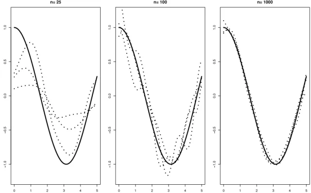
The model.Let us consider the model

Yi

=

f0

(

Xi)

+

εi

where

εi

∼

i.i.d.Unif

(

−

1

,

1

),

Xi

∼

i.i.d.Unif

(

0

,

5

),

fori

∈ {

1

, . . . ,

n

}

and

f0

(

x

)

=

cos

(

x

),

x

∈

R

.

The simulation consists of 5000 runs of this model where, in each run, data sets of sizen

=

25,n

=

100, andn

=

1000 were simulated.

Estimation.For the estimation, the SVM with the Gaussian RBF kernelk

(

x

,

x′

₎

₌

_exp

₍

₋

₍

_x

₋

_x′

₎

2

₎

_{and the (rescaled) logistic}

loss function L

(

x

,

y

,

t

)

= −

1 2

·

log



4 exp

(

−

2

(

y

−

t

))



1

+

exp

(

−

2

(

y

−

t

))



2



,

x

,

y

,

t

∈

_R

,

were used. Furthermore,

λ

0

=

0

.

0001 was fixed and, for each data set, the empirical regularization parameter

λ

Dn was

chosen in a data-driven way by a 5-fold cross-validation within the values 0

.

0001

,

0

.

0005

,

0

.

001

,

0

.

005

,

0

.

01

,

0

.

05

,

0

.

1

.

The theoretical SVMfL,P,λ0nearly coincides with the true regression functionf0; the absolute difference

|

fL,P,λ0

(

x

)

−

f0

(

x

)

|

is

smaller than 0.03 for everyx

∈ [

0

,

5

]

and theL1-distance betweenfL,P,λ0andf0is approximately equal to 0.002.

Results.As an example,Fig. 1shows the estimated functionfL,Dn,λDnof the first three runs for everyn

∈ {

25

,

100

,

1000

}

respectively. Note that SVMs using Gaussian kernels are a non-parametric method and, accordingly, larger sample sizes (such as e.g.n

=

1000) are needed in order to get fairly accurate estimates. Nevertheless, it turns out that approximate normality of

√

n



fL,Dn,λDn

−

fL,P,λ0



is present even for small sample sizes in this example. By fixingx0

=

2

.

5, for everyn

∈ {

25

,

100

,

1000

}

,

we obtain 5000 real numbersrn,j

:=

√

n



fL,Dn,j,λ_Dn_,j

(

x0

)

−

fL,P,λ0

(

x0

)



— wherej

∈ {

1

, . . . ,

5000

}

denotes the number of the run — in the 5000 runs. According toTheorem 3.1, the real numbersrn,j,j

∈ {

1

, . . . ,

5000

}

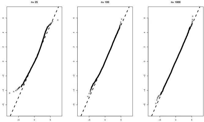
, are from an approximate normal

distribution if the sample sizenis sufficiently large.Fig. 2shows a histogram of the numbersrn,j,j

∈ {

1

, . . . ,

5000

}

, for

everyn

∈ {

25

,

100

,

1000

}

. In addition,Fig. 3shows, for everyn

∈ {

25

,

100

,

1000

}

, a Q–Q plot in which the empirical distribution of the numbersrn,j,j

∈ {

1

, . . . ,

5000

}

, is compared to the normal distribution with mean equal to the sample

mean ₅₀₀₀1



5000

j=1 rn,jand standard deviation equal to the sample standard deviation ofrn,j,j

∈ {

1

, . . . ,

5000

}

. Particularly Fig. 3illustrates that the numbersrn,j,j

∈ {

1

, . . . ,

5000

}

are approximately normal even for small sample sizes. Finally, Table 1shows the sample mean and the sample standard deviation ofrn,j,j

∈ {

1

, . . . ,

5000

}

, for everyn

∈ {

25

,

100

,

1000

}

.

In addition,Table 1shows the values of the Kolmogorov–Smirnov distance (KS-distance) between the empirical distribution function and the respective normal distribution function.

(8)

Fig. 1. The true regression functionf0 : x→ cos(x)(solid line) and the estimated functionsfL,Dn,λDnof the first three runs (dotted lines) for every n∈ {25,100,1000}respectively.

Fig. 2. For everyn∈ {25,100,1000}, a histogram of the numbersrn,j:=

√

n

fL,Dn,j,λDn,j(x0)−fL,P,λ0(x0) 

,j∈ {1, . . . ,5000}.

3.3. Supplements and sketch of the proof

The proof ofTheorems 3.1and3.2is an involved application of the functional delta-method. In order to describe this in some more detail, let us first fix a constant sequence of regularization parameters. That is,

λ

Dn

≡

λ

0

∈

(

0

,

∞

)

for

everyn

∈

_N. Then, support vector machines may be represented by a functionalSon a set of probability measures on



X

×

Y

,

B

(

X

×

Y

)



. This functional

(9)

Fig. 3. For everyn∈ {25,100,1000}, a Q–Q plot in which the empirical distribution of the numbersrn,j,j∈ {1, . . . ,5000}, is compared to the normal distribution with mean equal to the sample mean and standard deviation equal to the sample standard deviation ofrn,j,j∈ {1, . . . ,5000}.

is calledSVM-functionalin the following. It represents the SVM-estimator because the empirical support vector machine is equal tofL,Dn,λ0

=

S

(

PDn

)

for every data setDn

∈

(

X

×

Y

)

nwherePDndenotes the empirical measure corresponding toDn.

In order to use the functional delta-method, it is crucial that this is true for every sample sizenand thatSdoes not depend onn. (InRemark 3.7, it will be explained how it is nevertheless possible to deal with random sequences

λ

Dn.)Theorem 3.1

can be shown in the following way:

1. Show that

√

n

(

_PDn

−

P

)

converges weakly to a Gaussian process.

2. Show thatSis Hadamard-differentiable: (a) Show thatSis Gâteaux-differentiable.

(b) Show that the Gâteaux-derivative fulfills a continuity property. (c) Show that (a) and (b) imply Hadamard-differentiability. 3. Then, it follows from the functional delta-method that

√

n

(

fL,Dn,λ0

−

fL,P,λ0

)

=

√

n



S

(

PDn

)

−

S

(

P

)



converges weakly to a Gaussian process.Theorem 3.2follows fromTheorem 3.1by another application of the functional delta-method.

Step 1 involves the study of Donsker classes. Among other things, this is based on a bound(62)on the uniform entropy number of balls in the reproducing kernel Hilbert spaceH. A proof of this bound is given in the proof ofLemma A.9. In similar settings, such bounds have already been proven, e.g., in [37, Section V] and [29, Section 6.4]. In general,

√

n

(

PDn

−

P

)

isnota

measurable random variable so that the proof involves the theory of weak convergence of unmeasurable random variables; see [35]. However, this does not affect the statements ofTheorems 3.1and3.2because

ω

→

fL,Dn(ω),λDn(ω) is a measurable

random variable as shown in the beginning of the proof ofTheorem 3.1inAppendix A.4.

Essentially, it has already been known thatSis Gâteaux-differentiable because [8,7] derive the influence function ofS

which is a (special) Gâteaux-derivative. Therefore, essential steps of the proof of Step 2(a) can be adopted from [8,7] and [29, Section 10.4] but some care is needed as we also have to deal with signed measures here. In addition, we also have to deal with a sequence of random regularization parameters

λ

Dninstead of a fixed

λ

0; seeRemark 3.7. In Step 2(c) it will be shown

thatSis even Hadamard-differentiable (in a specific sense described inAppendix A.3). This is done because the application of the delta-method requires Hadamard-differentiability. However, this might also be useful for other purposes since, e.g., the chain rule is valid for Hadamard-differentiability but not for Gâteaux-differentiability. [9] shows Bouligand-differentiability of the SVM-functional which also allows the chain rule.

(10)

Remark 3.7 (Sequences of Random Regularization Parameters

λ

Dn).For a fixed regularization parameter

λ

0, support vector

machines can be represented by a functionalS

:

P

→

fL,P,λ0and the delta-method can be applied forS. However, if we have

a sequence of (random) regularization parameters

λ

Dn, we get a (random) sequence of functionals. SDn

:

P

→

fL,P,λDn

for which the delta-method cannot be applied offhand. This problem can be solved in the following way: As described in

Appendix A.1, SDn

(

P

)

=

fL,P,λDn

=

fL,λ0 λDnP,λ0

=

S



λ

0

λ

Dn P



∀

P

.

so that everything can be traced back toS. In this way, the explicit use ofSDncan be avoided and the delta-method turns out

to be applicable also in this case. The price we have to pay is that we have to deal with general finite measures in the proofs because, in general,_λDλ0

n(ω)Pis not a probability measure any more.

4. Conclusions

In the article, asymptotic properties of support vector machines are investigated. For sequences of random regularization parameters

λ

Dn,n

∈

N, such that

√

n



λ

Dn

−

λ

0



−→

0 in probability, it is shown that the difference between the empirical and the theoretical SVM is asymptotically normal with rate

√

n; that is,

√

n

(

fL,Dn,λDn

−

fL,P,λ0

)

converges to a Gaussian process

in the function spaceH. The value

λ

0

>

0 corresponds to a bound on the complexity of the estimate for the regression

function; a smaller

λ

0allows for more complex functions. Therefore, the theoretical SVMfL,P,λ0 serves as a ‘‘smoother’’

approximation of more complex regression functions. The results of this article show that, in non-parametric classification and regression problems, the estimation of this smoother approximation by use of empirical SVMs in an infinite dimensional function space is asymptotically normal with rate

√

n— just as if it was a parametric problem. The proof is done by showing that the mapP

→

fL,P,λis suitably Hadamard-differentiable and by an application of a functional delta-method. These results

are not only of theoretical interest but may also be a starting point for statistical inferences such as confidence intervals and hypothesis testing.

Estimating a smoother approximation of the regression function is a comprise between a parametric model and a fully non-parametric model without any assumptions on the regression function or the distribution. Without any of such assumptions, similar results are not possible as follows from the no-free-lunch theorem.

Acknowledgments

I would like to thank Andreas Christmann for bringing the problem to my attention and for valuable suggestions.

Appendix. Proof of the main results

The assumptions ofTheorem 3.1are valid in the whole appendix.

A.1. Preparations

The mapΦ

:

X

→

Halways denotes the canonical feature map corresponding to the kernelkand the RKHSH. It will frequently be used in the proofs that the reproducing property implies

⟨

Φ(x

),

f

⟩

_H

=

f

(

x

)

∀

x

∈

X,

∀

f

∈

H (15)

or, in shorter notation,

⟨

Φ,f

⟩

_H

=

f

∀

f

∈

H

.

(16) In particular, we write Eµ

⟨

Φ,f

⟩

_H

=



⟨

Φ,f

⟩

_Hd

µ

=



⟨

Φ(x

),

f

⟩

Hµ(dx

)

=



f

(

x

)µ(

dx

).

(17)

According to [29, p. 124], boundedness ofkimplies:

∥

k

∥

∞

:=

sup x∈X



k

(

x

,

x

)

=

sup x∈X

∥

Φ(x

)

∥

_H

<

∞

(18)

∥

f

∥

∞

≤ ∥

k

∥

∞

· ∥

f

∥

H

∀

f

∈

H

.

(19)

(11)

In order to shorten notation, define

Lf

:

X

×

Y

→

R

, (

x

,

y

)

→

Lf

(

x

,

y

)

=

L



x

,

y

,

f

(

x

)



for every functionf

:

_X

→

_R. Accordingly, define

L′_f

(

x

,

y

)

=

L′



x

,

y

,

f

(

x

)



and L′′_f

(

x

,

y

)

=

L′′



x

,

y

,

f

(

x

)



for every

(

x

,

y

)

∈

X

×

Y. AsLis aP-square-integrable Nemitski loss function of orderp

∈ [

1

,

∞

)

, there is ab

∈

L2

(

P

)

such

that

|

L

(

x

,

y

,

t

)

| ≤

b

(

x

,

y

)

+ |

t

|

p

∀

(

x

,

y

,

t

)

∈

X

×

Y

×

_R

.

(20) Let G1

:=



g

:

X

×

Y

→

_R

| ∃

z

∈

_Rd+1such thatg

=

I₍−∞,z]



be the set of all indicator functionsI₍−∞,z]. Then, it is well-known that

√

n



Fn

−

F



❀G1 in

ℓ

∞

(

G1

),

where_Fndenotes the empirical process,F denotes the distribution function ofP,G1 is a Gaussian process, and

ℓ

∞

(

G1

)

denotes the set of all bounded functionsG

:

G1

→

R. Provided that the SVM-functionalSis Hadamard-differentiable in

ℓ

∞

(G

1

)

, an application of the functional delta-method would yield asymptotic normality of

√

n



S

(

Fn)

−

S

(

F

)



. Unfortunately,

the norm-topology of

ℓ

∞

(

G1

)

is too weak in order to ensure Hadamard-differentiability. Therefore, the set of indicator

functionsG1has to be enlarged to a setG

⊃

G1which leads to the following somewhat technical definition of the domain BSof the SVM-functionalS. Define

c0

:=



1

λ

0



b dP

+

1

,

(21) G2

:=







g

:

X

×

Y

→

_R



∃

f0

∈

H

,

∃

f

∈

Hsuch that

∥

f0

∥

H

≤

c0

,

∥

f

∥

H

≤

1 and g

=

L′_f 0f







,

and G

:=

G1

∪

G2

∪ {

b

}

.

Let

ℓ

∞

(

G

)

be the set of all bounded functions

F

:

G

→

_R

with norm

∥

F

∥

∞

=

supg∈G

|

F

(

g

)

|

. Define

BS

:=











F

:

G

→

_R



∃

µ

̸=

0 a finite measure onX

×

Ysuch that

F

(

g

)

=



gd

µ

∀

g

∈

G

,

b

∈

L2

(µ),

b′a

∈

L2

(µ)

∀

a

∈

(

0

,

∞

)











andB0

:=

cl



lin

(

BS

)



the closed linear span ofBSin

ℓ

∞

(G)

. That is,BS is a subset of

ℓ

∞

(G)

whose elements correspond to

finite measures. The elements ofBScan be seen as some kind of generalized distribution functions. Note that the assumptions

onLandPimply thatG

→

_R

,

g

→



gdPis a well-defined element ofBS.

For everyF

∈

BS, let

ι(

F

)

denote the corresponding finite measure

µ

on



X

×

Y

,

B

(

X

×

Y

)



such that

F

(

g

)

=



gd

µ

∀

g

∈

G

.

Note that, by definition ofBS,

ι(

F

)

uniquely exists for everyF

∈

BSso that

ι

:

BS

→

ca+

(

X

×

Y

,

B

(

X

×

Y

)),

F

→

ι(

F

)

is well-defined where ca+

₍

_X

_×

_Y

_,

_B

₍

_X

_×

_Y

₎₎

_{denotes the set of all finite measures on}

₍

_X

_×

_Y

_,

_B

₍

_X

_×

_Y

₎₎

_{. The set of all finite} signedmeasures on

(

X

×

Y

,

B

(

X

×

Y

))

is denoted by ca

(

X

×

Y

,

B

(

X

×

Y

))

. The set of all continuous functionsf

:

X

→

_R

is denoted byC(X). SinceXis compact by assumption, the elements ofC(X)are bounded andC(X)is endowed with the sup-norm

∥

f

∥

∞

=

supx∈X

|

f

(

x

)

|

.

By now, support vector machines are only defined for probability measuresP

˜

. However, in order to deal with sequences of random regularization parameters

λ

Dn, we will also have to deal with ‘‘support vector machines’’ for general finite

measures

µ

. For everyF

∈

BS, define

fL,ι(F),λ

:=

arg inf f∈H



(12)

Though

µ

:=

ι(

F

)

∈

ca+

(

X

×

Y

,

B

(

X

×

Y

))

is not necessarily a probability measure, we have, in effect, not defined any new object. In order to see this, note that dividing the objective function byM

:=

µ(

X

×

Y

)

does not change the minimizer so that we get fL,µ,λ

=

arg inf f∈H



L



x

,

y

,

f

(

x

)



1 M

µ



d

(

x

,

y

)



+

λ

M

∥

f

∥

2 H

=

fL,_M1µ,_Mλ andf_L_,1

Mµ,Mλ is an ‘‘ordinary’’ support vector machine as 1

M

µ

is a probability measure. This also shows thatfL,µ,λuniquely

exists becausef_L_,1

Mµ,Mλ uniquely exists for the probability measure 1

M

µ

according to [29, Lemma 5.1 and Theorem 5.2].

The idea is that considering support vector machines for general finite measures

µ

makes it possible to take

λ

0as a

‘‘standard regularization parameter’’. Define

S

:

BS

→

H

,

F

→

S

(

F

)

=

fι(F)

,

where f_ι(F)

:=

fL,ι(F),λ0

=

arg inf f∈H



L



x

,

y

,

f

(

x

)



ι(

F

)



d

(

x

,

y

)



+

λ

₀

∥

f

∥

2H.

Then, we can deal with other regularization parameters

λ >

0 by use of

fL,ι(F),λ

=

S



λ

0

λ

F



∀

F

∈

BS

.

(22)

This is important in order to apply the functional delta-method in case of a sequence of random regularization parameters

λ

Dn; see alsoRemark 3.7.

It follows from [29, Eq. (5.4) and Lemma 4.23] that



fι(_F)



H

≤



1

λ

0 F

(

b

)

∀

F

∈

BS

,

(23)



fι(_F)



∞

≤ ∥

k

∥

∞



1

λ

0 F

(

b

)

∀

F

∈

BS

.

(24)

SinceXis separable andkis a continuous kernel, the RKHSHis aseparableHilbert space; see [29, Lemma 4.33]. Separability ofHis used several times in the proofs; this is important particularly with regard to the Bochner-integral ofH-valued functionsΨ

:

Z

→

H. The Bochner-integral



Ψd

µ

=



Ψd

µ

+

−



Ψd

µ

−of such aH-valued functionΨ with respect to a finite signed measure

µ

=

µ

+

₋

_µ

−_{is again an element of}_H_{. If}_Ψ _{is suitably measurable, then existence of the}

Bochner-integral follows from



∥

Ψ

∥

_Hd

|

µ

|

<

∞

where

|

µ

| =

µ

+

₊

_µ

−_{denotes the total variation of}

_µ

_{. We will also frequently use}

the fact that, for every Banach spaceEand every continuous linear operatorA

:

H

→

E, the existence of the Bochner-integral



Ψd

µ

implies the existence of the Bochner-integral



A

(Ψ

)

d

µ

and



A

(Ψ

)

d

µ

=

A



Ψd

µ



;

(25)

see, e.g. [11, Theorem 3.10.16 and Remark 3.10.17].

This subsection closes with three lemmas which are used several times. Thereafter, Gâteaux-differentiability of the SVM-functionalS

:

BS

→

Hwill be shown inAppendix A.2. This is strengthened to Hadamard-differentiability inAppendix A.3.

Finally, it will be shown inAppendix A.4that

√

n

(

PDn

−

P

)

converges weakly to a Gaussian process in

ℓ

∞

(

G

)

and that this

implies asymptotic normality of

√

n



fL,Dn,λDn

−

fL,P,λ0



and

√

n



RL,P

(

fL,Dn,λDn

)

−

RL,P

(

fL,P,λ0

)



by applying a functional delta-method.

Lemma A.1.Let

(

Fn)n∈N

⊂

BSbe a sequence which converges to some F0

∈

BS. Then,limn→∞

ι(

Fn)(X

×

Y

)

=

ι(

F0

)(

X

×

Y

)

and the sequence of finite measures

ι(

Fn), n

∈

_N, converges weakly to

ι(

F0

)

.

Proof. DefineMn

:=

ι(

Fn)(X

×

Y

)

andan

=

(

n

, . . . ,

n

)

∈

Rd+1for everyn

∈

N

∪ {

0

}

. Then,

0

≤ |

Mn

−

M0

| =

lim l→∞



F_n



I₍−∞,al]



−

F0



I₍−∞,al]





≤ ∥

F_n

−

F₀

∥

_∞

−→

0

.

Therefore, the normalized sequenceF

˜

n

=

Mn−1Fn,n

∈

N

∪ {

0

}

, corresponds to a sequence of probability measures

ι(

F

˜

n)such

that lim n→∞

ι(

˜

Fn)



(

−∞

,

a

] ∩

X

×

Y



=

lim n→∞ 1 Mn Fn



I₍−∞,a]



=

1 M0 F0



I₍−∞,a]



=

ι(

F

˜

0

)



(

−∞

,

a

] ∩

X

×

Y

