San Jose State University
SJSU ScholarWorks
Master's Projects Master's Theses and Graduate Research
Spring 6-1-2016
Supervised Learning for Multi-Domain Text
Classification
Siva Charan Reddy Gangireddy
San Jose State University
Follow this and additional works at:https://scholarworks.sjsu.edu/etd_projects Part of theArtificial Intelligence and Robotics Commons
This Master's Project is brought to you for free and open access by the Master's Theses and Graduate Research at SJSU ScholarWorks. It has been accepted for inclusion in Master's Projects by an authorized administrator of SJSU ScholarWorks. For more information, please contact [email protected].
Recommended Citation
Gangireddy, Siva Charan Reddy, "Supervised Learning for Multi-Domain Text Classification" (2016).Master's Projects. 483. DOI: https://doi.org/10.31979/etd.yvh3-uzqb
Supervised Learning for Multi-Domain Text Classification
A Writing Project Report Presented to
The Faculty of the Department of Computer Science San Jose State University
In Partial Fulfillment
Of the Requirements for the Degree Master of Science
By
Siva Charan Reddy Gangireddy May 2015
© 2015
Siva Charan Reddy Gangireddy ALL RIGHTS RESERVED
The Designated Project Committee Approves the Project Titled
Supervised Learning for Multi-Domain Text Classification
By
Siva Charan Reddy Gangireddy
APPROVED FOR THE DEPARTMENTS OF COMPUTER SCIENCE
SAN JOSE STATE UNIVERSITY
MAY 2015
Dr. Melody Moh (Department of Computer Science) Dr. Teng Moh (Department of Computer Science)
ABSTRACT
Digital information available on the Internet is increasing day by day. As a result of this, the demand for tools that help people in finding and analyzing all these resources are also growing in number. Text Classification, in particular, has been very useful in managing the information. Text Classification is the process of assigning natural language text to one or more categories based on the content. It has many important applications in the real world. For example, finding the sentiment of the reviews, posted by people on restaurants, movies and other such things are all applications of Text classification. In this project, focus has been laid on Sentiment Analysis, which identifies the opinions expressed in a piece of text. It involves categorizing opinions in text into categories like 'positive' or 'negative'. Existing works in Sentiment Analysis focused on determining the polarity (Positive or negative) of a sentence. This comes under binary classification, which means classifying the given set of elements into two groups. The purpose of this research is to address a different approach for Sentiment Analysis called Multi Class Sentiment Classification. In this approach the sentences are classified under multiple sentiment classes like positive, negative, neutral and so on. Classifiers are built on the Predictive Model, that consists of multiple phases. Analysis of different sets of features on the data set, like stemmers, n-grams, tf-idf and so on, will be considered for classification of the data. Different classification models like Bayesian Classifier, Random Forest and SGD classifier are taken into consideration for classifying the data and their results are compared. Frameworks like Weka, Apache Mahout and Scikit are used for building the classifiers.
iii
ACKNOWLEDGEMENTS
I would like to thank Dr. Melody Moh for believing in me and being my project advisor. Her guidance and encouragement supported me a lot throughout this project. I would like to convey my sincere thanks to my committee member Dr. Teng-Sheng Moh for his continuous guidance and support. Also, I would like to thank Mr. John Cribbs for being my committee member and for spending his valuable time in monitoring my project progress. Finally, I am very thankful to my family and friends for their encouragement.
iv TABLE OF CONTENTS CHAPTER 1 Introduction ... 1 2 Background ... 3 3 Problem ... 7 3.1Data ... 7 4 Proposed Solution ... 10
4.1Architecture for Proposed Solution ... 10
4.2Data Pre-Processing ... 11 4.2.1 Data Validation ... 11 4.2.2 Data Cleaning ... 12 4.2.3 Data Sampling ... 12 4.3Feature Selection ... 15 4.3.1 Bag of Words ... 16 4.3.2 Stopwords ... 17 4.3.3 Stemming ... 18 4.3.4 N-grams ... 19 4.4Predictive Model ... 21
v
4.5.1 Naive Bayes Model ... 23
4.5.2 Random Forest Model ... 30
4.5.3 Stochastic Gradient Descent Model ... 32
5 Experiments and Results ... 35
5.1Single tier results ... 35
5.1.1 Naive Bayes using Mahout ... 35
5.1.2 Random Forest using Scikit ... 38
5.2Multi tier results ... 41
5.2.1 Stochastic Gradient Descent using Scikit ... 41
1 CHAPTER 1
Introduction
The digital information available on the internet is growing day by day. Human intervention is not at all sufficient to analyze all this data. Many techniques are required to extract all this data, analyze it and draw meaningful patterns. Text classification is a machine-learning technique, in which the text is classified into different categories by different classification algorithms. Every classifier has its own way of gathering the features and using them in order to classify the text. Text classification has wide range of applications like spam filtering, genre categorization, language identification, routing the emails, sentiment analysis and many such applications. All these applications use wide range of text classification techniques.
Now-a-days sentiment classification is widely used by the businesses to know their brand value and to gain business intelligence. Feedback given by the customers about businesses is of great importance to them. Using the text from the feedback(reviews), the data can be mined for various interesting facts which might be helpful in increasing the market for a particular business. Mining the text might be of high importance when compared to the star rating system, because sentiment of the customer can't be seen in the latter. A particular user might give a business 3 star rating, but the review written by that user might not match with the star rating given. In this manner, sentiment classification has gained huge importance in the business world.
In this Project, supervised learning is the learning approach that has been adapted by the classifiers. In supervised learning, the training dataset consists of the data instances along with the labels provided for them. Initially the classifiers learn the data in a supervised fashion and then the model is evaluated with the data instances(test set) that doesn't consist of labels. The classifier, during evaluation, outputs the labels for testing instances and then the accuracies are computed. Dataset for this project is a corpus of movie
2
reviews obtained from rotten tomatoes website. Some pre-processing tasks are performed to split the data into train and test sets.
Many features like stop-words, stemmers, n-grams, parts of speech tagging have been used on this dataset for the classification task. Models like Bayesian, Random Forest and Stochastic Gradient Descent have been tried on this dataset for classifying the reviews under different labels.
This paper is organized as follows. The background research work that has been done to explore various methods and models are described in Section 2. Problem and the dataset structure is discussed in Section 3. In Section 4, the proposed approach is explained and finally the paper is concluded in Section 5.
3 CHAPTER 2
Background
Extracting the sentiment or opinion from a message or blog post is the typical way of obtaining the valuable information. Machine Learning Technologies are mainly used in the domain of sentiment classification for learning the model and then for prediction. ML Libraries like Mahout internally comprises of many machine learning algorithms and the usage of such technologies doesn't give us the complete control on the underlying ML Algorithms.
The idea proposed on implementing a Naive Bayes Classifier on the top of Hadoop framework, for classification of sentiment in [1], gives the authors, a fine grained control on the algorithm to accommodate high scalable data. The idea proposed in [1], is evaluated against million review sentences and the throughput seems to be efficient. Now-a-days spam is the major problem and spam categorization has got huge importance. There are many machine learning algorithms which distinguishes the spam mail from legitimate mail. The authors of [2], have tried several classifiers and classification approaches as well on the data set. Several measures and parameters which play a key role in spam categorization have also been specified in [2]. Analysis of different supervised classifiers using different data mining tools like Weka, Rapid Miner is shown; in [2].
Click Prediction plays a very major role in sponsored search system. Most of the research works on click prediction focused on the relevance information (similarity between ad and query) and the historical data of users click information. The authors in [3], proposed a new perspective of looking at click prediction. They mainly concentrated on the reasons behind a user clicking a particular ad. Tags like 'x% off', 'official site' increase the tendency of a user clicking a particular ad, is what the authors of [3] believed in. They proposed a system according to Maslow's desire theory, in which the users psychological desire is categorized under five levels. Clustering algorithm and Maximum Entropy
4
Modeling are used in this system. Evaluation is done for Rich history Ads Vs Rare history Ads and effects of desire level combinations over desire patterns.
Word Clouds are the most effective way of visualizing the text, as the words in the text are shown in a way as if their frequency is proportional to the font size. Usually this is done in a static way, meaning the summarization is done for static text. The authors of [4], have done research on the importance of word clouds for text analytics. A prototypical system called the word cloud explorer, into which the natural language processing techniques are integrated, have been developed in [4], and this completely relies on word clouds as the visualization method. Features like search, click based filter, part-of-speech filter, stop word editor and co-occurrence cloud have also been implemented in this system. They evaluated this system is such a way that is useful in qualitative study.
Data existing in social networking sites like Facebook, Twitter is very abundant and hence there is huge scope for extracting the emotional content from such data. The existing research works tend to identify the state of mind of users but are insufficient because of the ambiguity in the conveyed text. The authors of [5], have considered the Facebook posts during the 'Arabic Spring' era, for their research work. Their main idea is to extract the useful information from Tunisian users during this sensitive and significant period. A method that depends on Naive Bayes and SVM is proposed by them and several lexicons related to emoticons, interjections have been built to determine the sentiment of status updates.
Now-a-days illegitimate drug and cosmetic products are being developed in the market. Data mining might be helpful in this regard to eradicate such products. Hence there is a need for developing active surveillance system that reports the legitimacy of a drug or cosmetic product to the stake holders participating in anti-counterfeiting fight. The authors of [6], were involved in developing a framework for gathering and analyzing the user views using machine learning, text mining and sentiment analysis. The proposed framework was evaluated on Facebook comments and data from Twitter. Naive Bayes
5
Classification is used in [6], to develop a product safety lexicon and the model is trained with the facebook posts/ twitter tweets related to drug-cosmetic products.
Stock market is one among the key components of economy in most of the countries. In Stock market, there are various factors involved in making a decision. Lot of things like price trend, nature of the market, stability of the company, news related to a firm and rumors play a major role in making a decision. The idea of authors in [7], is to extract the fundamental information related to stocks from the news sources and use them in the analysis of stock market. They surveyed the existing business researches and proposed a framework which comprises of text parser and the analyzer as well. The system is evaluated, and this equipped framework is able to analyze and forecast the decisions from any data source.
Searching the existing research papers online is what most of the researchers do, in order to perform research on their areas of interest. Relevance really matters in this context, as the search results need to be really narrowed down in order to produce the specific results that are being expected. The authors of [8], proposed a classification system that uses the natural language processing techniques and k-means clustering algorithm for categorizing the research papers.
The model which determines the sentiment for a sentence in multiple stages is described in [16]. In this approach, the authors initially determine whether the sentence is polar or neutral. In the next level disambiguation is removed from polar sentences by classifying them into positive, negative or both. The authors in [17], followed three level hierarchical strategy for finding the sentiment of twitter data. In each and every level, the emotion is found and it is further fine-tuned in its lower level.
The approach of training the data in multiple layers with different set of features in every layer, is discussed by the authors in [18]. The performances at every layer are discussed and compared. The authors in [19], discusses a new strategy which finds the sentiment of text based on the results from multiple levels. Text is initially divided into small parts and
6
the sentiment is found for every part. Integrating the sentiment results of every part determines the sentiment of the actual text.
The above mentioned research from [16],[17],[18],[19] is the main motivation for proposing a multi-tier framework for sentiment classification. Some of the dictionary building techniques from [5], [6] have also been applied to the proposed model. The next section discusses about the data and classifiers that have been used for sentiment classification.
7 CHAPTER 3
Problem
Existing works in Sentiment analysis focused on determining the polarity (Positive or negative) of a sentence. This comes under binary classification, which means classifying the given set of elements into two groups, based on the sentiment they carry.
Multi-Class Sentiment Analysis or Multi-Labeled Sentiment Analysis is the data mining problem, that has been chosen for Text classification. This can be considered as a different problem under Sentiment Classification. In this problem the sentences are classified under multiple sentiment classes like positive, negative, neutral and so on. Dataset is the collection of movie reviews from Rotten Tomatoes website. The main agenda of this problem is to label the reviews under five values: negative, fairly negative, neutral, fairly positive and positive.
Data not only consists of review sentences, but also consists of phrases obtained from those review sentences, which makes this problem more challenging. Negation in sentences, ambiguity in the language and sarcasm also makes this challenging. The structure of the dataset is presented in the following section.
3.1 Data: Dataset:
Dataset consists of 5 Sentiment Labels
Negative (or) '0'
Fairly Negative (or) '1'
Neutral (or) '2'
Fairly Positive (or) '3'
8 Training Set consists of 156k instances
Testing Set consists of 66k instances
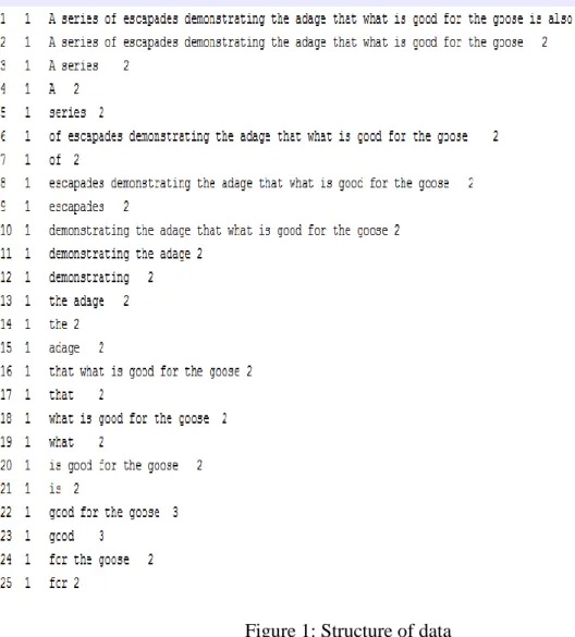
The attributes present in each instance are shown below in detail.
Figure 1: Structure of data
As shown above in the picture, each instance in the dataset is described by 4 attributes: PhraseId - The unique identifier(key) for each phrase in the dataset
9
Phrase - The review or a phrase obtained from that review Sentiment - The emotion that a review or phrase carries
Basically, the dataset consists of both reviews and the phrases obtained from those reviews.
For example:
If there is a review, "The movie is not that interesting", and if this is the first review in the dataset, then this is how it is uniquely identified in the dataset.
PhraseId SentenceId Phrase Sentiment 1 1 The movie is not that interesting 2
2 1 The movie 3
3 1 is 3 4 1 not that interesting 2
This is how, the dataset is organized with both the reviews and the phrases obtained from those reviews, using two identifiers, one which uniquely identifies the phrase and the other which uniquely identifies the review.
10 CHAPTER 4 Proposed Solution
4.1 Architecture for Proposed Solution:
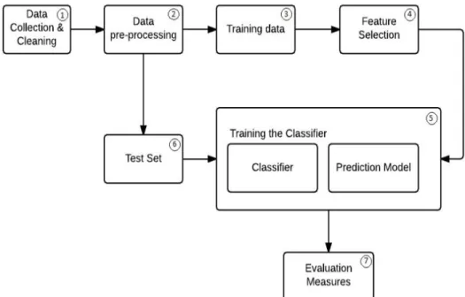
The process flow that has been followed to solve this problem of multi class sentiment classification is shown in the below picture.
Figure 2: Architecture for Proposed Model
Initially data is collected in the first phase and it is verified for any data outliers. All such noise is removed during the initial phase. During the pre-processing phase the data is transformed in such a way, that the machine learning algorithms directly work on the processed data. In this project, train and test sets are split during this phase.
Once the train set is obtained, features are selected from it during the Feature Selection phase. Features for this dataset are words and several techniques like stop-word removal,
11
stemming, n-grams are applied during this phase. Once this is done, the classifier is implemented in such a way that it adapts the Predictive Model, that consists of multiple phases. Classifier is then trained with the train set and the test set is applied to the classifier for the purpose of evaluation. Each of these phases are described in detail in the following sections.
4.2 Data Pre-Processing:
This can be considered as one of the most important steps to be performed before selecting the features from the dataset. The main agenda of this particular phase is to remove the unwanted data and retain only the data that is required for feature selection. This phase can be sub-divided into many other steps like data validation, data cleansing, data sampling and so on. The actions performed in each of these steps is discussed below in detail.
4.2.1 Data Validation:
In this step, some checks are performed to determine the validity of the dataset. The dataset is tested for:
NULL values: The dataset might consist of NULL values, which means for a particular instance, there might be a possibility of the review being empty. All such cases are tested using Hive queries after loading the dataset into Hive table. Some of those queries are shown below.
Validity of Sentiment labels: The valid range of sentiment labels for this dataset is [0,1,2,3,4]. There might be every possibility of a sentiment label being a value, not in the specified range. Hive queries are used to test this case, which is shown below.
12 4.2.2 Data Cleansing:
Data Cleansing or Data Scrubbing is the process of checking the inappropriate attributes from the dataset and removing them. In this particular dataset PhraseId, uniquely identifies each review and the phrase as well. So, the existence of SentenceId, might not be that important and this particular column can be removed from the dataset.
4.2.3 Data Sampling:
As discussed earlier the dataset consists of both train-set and test-set. The train-set consists of a valid Sentiment label for each and every instance. The test-set doesn't consist of a Sentiment label and that is what, is to be determined for the test-set. As, the test-set doesn't consist of Sentiment labels, accuracy of the model can't be determined. Therefore, the initial train-set is split into two parts with the split factor being 80:20, 80 for train-set and 20 for test-set.
Splitting should be done in such a way, that the Sentiment label distribution in the actual train-set should be properly maintained.
For example:
Initial Train-Set
Train Dataset (80%) Test Dataset (20%)13
If the data is randomly split and train set consists of labels (0,1,2,3), test set consists of labels (0,1,2,4), there is no way for the model to determine the label for instances with Sentiment '4', as it is not present in the train-set.
If the train-set consists of half of the instances with label '2', then there is every chance of the model being more biased towards label '2', while determining the sentiment for the instances in the test set.
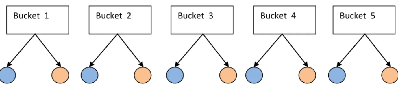
In order, to avoid these kind of scenarios, proper data sampling should always be maintained. 'Bucketing' feature in hive has been used to properly sample the data and maintain the label distribution ratio.
Using Hive Bucketing, the initial train dataset is split into five buckets. Bucket 1 - carries all the instances with label '0'
Bucket 2 - carries all the instances with label '1' Bucket 3 - carries all the instances with label '2' Bucket 4 - carries all the instances with label '3' Bucket 5 - carries all the instances with label '4'
Here is the Hive query used for performing the bucketing on initial data set.
After creating 5 buckets, each bucket is considered and divided into two parts, one comprising 80% of the random instances (shown in blue) from the chosen bucket and the other comprising remaining 20%(shown in orange) of the random instances.
14
Figure 3: Data Buckets and Sampling
Here is the sampling query used to divide each bucket into two parts
After executing this query on all the five buckets,
All the blue colored parts (80% of instances from particular bucket) shown in the above diagram are merged to form the properly sampled train-set.
All the orange colored parts (20% of instances from particular bucket) are merged to form the properly sampled test-set.
By the end of this step, train-set (125k) and test-set (30k) with proper label distributions are obtained.
15 4.3 Feature Selection:
Feature selection is the process of selecting the features that are most essential and that are more relevant to the machine learning problem, which is being considered. To further simplify, in the context of Text classification, only the features that help in determining the sentiment of a sentence are to be considered.
In Sentiment classification, words play a major role in determining the sentiment of a sentence. Hence, words are said to be the features in the context of Text classification. There are many advantages in performing the feature selection before building the classifier and modeling the data.
Accuracy might improve: When the relevant features are only selected for modeling, there is every chance for the accuracy to get improved.
Training time is reduced: After removing all the unwanted features, it is very obvious that the training time is reduced.
Over-fitting gets reduced: When the redundant data is less, there is very less probability for the model to make decisions based on noise.
In this project, for the dataset that is being considered, there are 14k unique words, that are being considered as the features for the machine learning model. Furthermore, features like stop-word removal, stemming, n-grams and so on, will also be considered for further fine tuning before modeling the data.
The set of such features used in this project will be discussed in detail in the following sections.
16 4.3.1 Bag of Words:
Bag of words model is widely used in many of the text classification applications such as spam filtering and document classification. In this model, text such as review or document is considered as a bag of words. The grammar is disregarded and even the order of words is ignored, but the multiplicity of the word is considered.
In this project, after considering each review as a bag of words, multiplicity(frequency) of each word is considered as a feature while training the classifier. The model shown below gives an overview of how this works.
For example, consider two reviews: 1) The movie is not that interesting
2) The movie is a thriller and its worth watching
Based on these two reviews, a dictionary is created as shown below { "The" : 1, "movie" : 2, "is" : 3, "not": 4, "that": 5, "interesting": 6, "a": 7, "thriller": 8, "and": 9, "its": 10, "worth" : 11, "watching" : 12
17 }
These two reviews have 12 words altogether and by using the indexes from dictionary, these two reviews can be represented in the feature space as shown below
[1,1,1,1,1,1,0,0,0,0,0,0] [1,1,1,0,0,0,1,1,1,1,1,1]
In this way, all the reviews can be represented in the vector space and the classifier can use this feature for training the model.
4.3.2 Stop-words:
In the case of sentiment classification, after considering words as the features for training the classifier, there are still some words which don't play any role in deciding the sentiment of a particular sentence [9].
In the dataset used for this project, some of the words like
{in, the, anywhere, are, around, as, at, be, became, because, become, been, being, between, both,
but, by, can, could, detail, each, either, else, elsewhere, etc, even,...}
and many more such words doesn't determine the sentiment of a particular review [10]. So, removing all such words will be advantageous in many ways like:
Storage space of the feature vector decreases.
Performance of the classifier increases, which means it's running time decreases.
There is every chance for the accuracy to improve.
18
Many API's provide stop words list, which can be used directly or customized stop-words can be added into the existing lists based on the context.
In this project, some words from the reviews like {' -LRB-', '-RRB-', '$',...} are added to the existing stop-word lists for better performance.
4.3.3 Stemming:
Stemming is the process of removing the suffix from a word. Stemming is widely used in search engines for expanding a query, indexing and natural language processing [11]. The algorithms which does stemming are called stemmers or stemming algorithms. There are many stemming algorithms like
Porter's stemmer
Lovins Stemmer
Iterated Lovins Stemmer
Null Stemmer
Each of these differs in the performance and the context to be used as well. Stemmers basically removes the 'ing' form, 'ly' form and 'ed' form from the words.
19
In the dataset used for this project, in many of the reviews there are words like 'lovely', 'badly' and so on. 'lovely' becomes 'love' and 'watching' becomes 'watch' after a stemmer is applied.
Stemming has been used in this project before the data is pipelined to the classifier. For example, if there are two reviews
Star cast performances are very bad and so it's better to skip the movie.
Climax has badly affected this movie.
While the feature vectors are built for these two reviews, the words 'bad' and 'badly' will be treated as two separate words. Because of this, multiplicity(frequency) of these two words are calculated separately.
If stemming is applied on this corpus, 'badly' is treated as 'bad', and only 'bad' will have an entry in the dictionary of the classifier with word frequency 2.
Thus the advantages of this technique are:
Storage space of the feature vector decreases
The probability of a word falling into a particular sentiment dictionary gets increased
When stemming is applied on this dataset, there is a significant improvement in the accuracy, which will be discussed in the later sections.
4.3.4 N-grams:
N-grams are widely used in many areas of computer science. N-grams are 'n' contiguous words from a given sentence [12]. If the size of the n-gram is 1, then it is referred as 'unigram', similarly a 'bigram' if the size is 2, and a 'trigram' if the size is 3.
For example, if a review is considered "The movie is worth watching"
20
Here is the unigrams, bigrams and trigrams list for this particular review. Unigrams: {'The', 'movie', 'is', 'worth', 'watching'}
Bigrams: {'The movie', 'movie is', 'is worth', 'worth watching'} Trigrams: {'The movie is', 'movie is worth', 'is worth watching'}
While predicting the sentiment for a review, n-grams might be very useful. For instance, in this example, the bigram 'worth watching' is clearly helpful for the classifier to predict this review as a positive one.
In the same manner, under different contexts, n-grams with different sizes will be very useful for the classifier to perform accurate predictions. Usage of n-grams might improve the accuracy as well.
In this project, n-grams with different sizes are applied to the dataset along with the previously mentioned features. For this particular dataset, bigrams worked effectively when compared relatively to unigrams and trigrams. This is because, generally most of the reviewers strongly express their opinion about a movie in two contiguous word combinations like 'very good', 'worth watching', 'utterly failed' and this might be the reason for bigrams working more effectively on this dataset.
The accuracies varied a bit upon applying n-grams with different sizes on this dataset. This will be shown in the later sections under a particular classifier, when n-grams is tried along with other features discussed above.
21 4.4 Predictive Model:
In section 4.1, the architecture for the proposed model has been discussed. The role of predictive model while building the classifier is discussed in detail here.
Figure 4: Architecture of Predictive Model
This Predictive Model consists of multiple phases. During each and every phase the classifier is trained with different instances. Each and every phase is explained below. Phase I:
During this phase, the classifier is trained with the data that consists of three labels. (Negative + Fairly Negative) instances are considered under label '0'
Neutral instances are considered under label '2'
22
Whenever a test instance is applied to this phase, the classifier outputs any of these labels [0,2,4]. Based on the label that is predicted by the classifier, the remaining steps in the process flow takes place.
If the label predicted by the classifier is '2', then both the phraseId and predicted label are printed in the result file.
If the label predicted by the classifier for test instance is '0', Phase II is executed and if the predicted label is '4', Phase III is executed.
Phase II:
During this phase, the classifier is trained with the data that consists of two labels. Negative instances are considered under label '0'
Fairly Negative instances are considered under label '1'
The test instance applied during the Phase I, is predicted as either '0' or '1' during Phase II. Once the prediction is done, phraseId and predicted label are printed in the result file. Phase III:
In phase III, the classifier is trained with the data that consists of two labels. Fairly Positive instances are considered under label '3'
Positive instances are considered under label '4'
In this phase the test instance coming from Phase I, is predicted as either '3' or '4'. After this phase the label along with the phraseId is sent to the result file.
Generally, a classifier predicts better when there are less number of labels during the classification task. This advantage is utilized in this predictive model during the execution of each phase. In the next section the classifiers used for classifying the data are discussed.
23 4.5 Classifier Selection and Parameter Tuning:
In this project, various classifiers have been chosen for classifying the dataset and their parameters are tuned to improve the accuracy.
4.5.1 Naive Bayes Model:
Bayes theorem, is the building block of Naive Bayes classifier and this particular classifier has got many variants [13]. This is widely used in many of the machine learning models, particularly in the areas of document classification, spam filtering and many such areas.
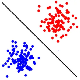
Naive Bayes classifier is linear, which means all the data samples can be separated by a line on the vector model, where each vector represents a sample. The adjective 'Naive' here indicates that all the features within the dataset are mutually independent. Some of the terms like posterior probability, class-conditional probability, prior probability play a key role in predicting the result for a particular instance.
Figure 5: Linear Classifier
24
Any classifier considers the features present within the dataset, which predicting the result. In this project as the reviews are being classified, the only features that any classifier considers during the training process are the words. As per the Bayes rule, all the words(features) are assumed to be mutually independent of each other. Words from all the reviews will be considered, their multiplicity will be maintained and a dictionary will be built before the classifier is trained with the train instances.
If we consider two reviews:
The movie is not that good : negative
Movie is good : positive
Here positive and negative are the sentiment labels(classes) for those two reviews. Class-conditional probability is a probability that a particular word, for example the word 'good' belongs to a particular class (say positive) in the above example. 'good' occurred twice(one time in negative and the other time in positive ) in the above reviews and hence the conditional probability of good occurring under 'positive' class is 0.5. Prior Probability is the probability that a particular class is encountered in the training samples. In this example, prior probability of 'negative' and 'positive' is 0.5.
To generalize, if w1, w2, w3, w4... wi are considered to be the words in the dictionary(bag of words) collected from all the data samples and Y1 Y2 Y3 Y4.... Yj are the classes present in the dataset, then conditional probability of a word w1 belonging to class Y1 is denoted as P(w1| Y1). Prior probabilities of Y1 is denoted by P(Y1) and likewise prior probability of a class Yj is denoted by P(Yj).
The Naive Bayes model that has been used for the reviews dataset is shown below: P(Y, w1, w2, w3, w4... wi) = P(Y) ∏i P(wi | Y)
Here w1, w2, w3, w4... wi are the features(words) occurring within a particular data instance and 'Y' indicates the class. In this dataset, there are about 13k words and 5 different sentiment labels.
25 P(Y)
4.5.2 Random Forest Model:
Random Forest follows an 'ensemble' learning approach. Random Forest can be used for classification, regression and other such tasks [14]. 'Ensemble' here refers to the collective decision making. The name itself indicates that this classifier is a collection of multiple decision trees. This classifier tries to avoid falling into the trap of 'over-fitting' for training set'. As, Random Forest is a collection of many decision trees, and as each tree behaves differently, there is more probability for this model to avoid over-fitting of train data.
Growing the trees in Random Forest Algorithm:
In this algorithm trees are grown in a top-down manner and the algorithm is explained below [15]:
Let 'N' be the total number of training samples used for training the classifier and 'M' be the total number of features available within the dataset that can be used by the classifier.
Out of 'M' features available, the classifier considers only 'm' features at each node of the tree while making a decision. m < M, generally 'm' is considered to be the square root of 'M', m = √M.
P(Y1) = P(negative)
P(Y2) = P(fairly negative)
P(Y3) = P(neutral)
P(Y4) = P(fairly positive)
26
Consider each decision tree and choose a training set for every tree, in such a way that all the available 'N' training samples are considered by that tree in 'n' times, considering a part of samples for finding the error estimate of the tree.
At every node in the tree, consider only the 'm' features from the available 'M', for making out a decision at that node. The best split at that node can be found based on these 'm' features.
Here are the tuning parameters for the Random Forest Model:
Trees being grown(n): The variable 'n' indicates the total number of trees taken into consideration for growing the Random Forest classifier. Now, as there are 'n' decision trees, the training samples are divided into 'n' training splits. Each training split will now be taken care by a decision tree and the rest of the samples can be used for finding the error estimate. In the case of test sample evaluation, the Random Forest Model follows 'Bagging approach', which means that the model takes the opinion of every decision tree and decides the majority vote as the value for test instance. In this project, trees ranging from 100-200 are considered for the Random Forest Classifier.
m-variables: This particular parameter indicates the random variables(features) chosen at every node in the tree while a decision is being made. If 'M' are considered to be the total features available, only 'm' random features are considered at every decision making point.
In this project, there are around 13k features available. This tuning parameter gives better results when m <= √13k (or) m <= 114
Rules for Tree splitting:
A Random Forest Tree can be split using some rules like Gini, Twoing and Entropy. Gini, does splitting by differentiating the instances with different labels. Gini rule, mainly concentrates on a particular label while separating all the instances related to that label. It is mainly biased towards the label with largest number of data instances.
27
Twoing, attempts to divide the labels into two separate groups, in such a way that each group accounts to half of the data. Further, this process takes place recursively until all the labels are separated. Entropy rule, also works somewhat similar to this. These tree splitting rules really makes difference in the case of large datasets. Gini has been used for this project.
4.5.3 Stochastic Gradient Model:
Stochastic Gradient Descent (SGD) is one more model that has been used in this project to predict the labels for reviews in the dataset. Scikit API provides this classifier under the category of linear models. This classifier has been successfully used to solve natural language processing problems. SGD classifier is used mainly to solve large scale text classification problems, as this model learns from every instance and immediately adjusts the objective function to minimize the error rate. This classifier can handle large number of features and as this problem of labeling the reviews, has many features involved, this has been chosen as one of the classifiers for solving this text classification problem. SGD is like an extension to Gradient Descent method.
Gradient Descent is usually a method which optimizes a function and finds the local minimum parameters for it. For example, if there is a linear function f(X) = Θ0+ Θ1X , gradient descent method finds the local minimum vales for Θ0 and Θ1. In the context of machine learning, if 'X' is considered to be a data instance(a review) and 'Y' is supposed to be the label(Sentiment) for it, then function f(X) which finds the label for data 'X' is treated as a hypothesis function. A loss function also called as cost function, maps a set of values to a value, which in the case of this dataset can treated as the mapping between the review(words as features) and its sentiment. Gradient Descent minimizes the loss function and tries to reduce the deviation between the actual label and the predicted label. Batch Gradient Descent is one variant of Gradient Descent, in which the former is called 'Batch' as it has got the functionality of handling many data samples.
28
How Batch Gradient Descent is different from Stochastic Gradient Descent:
If we assume the loss function to be L(Θ0,Θ1) and 'm' be the total number of instances(reviews) in the data set,
For Batch Gradient Descent, the pseudo code goes like this Repeat
{
Θj := Θj - α (L(Θ) for all the 'm' samples) (for every j = 0,....n)
}
Here for every value of 'j', the loss is computed for all the samples of 'm', which means the values of Θj change after all the 'm' samples are computed.
Pseudo-Code for Stochastic Gradient Descent:
1. Randomly shuffle the dataset. 2. Repeat
{
for i = 1,2,3...m {
(for every j = 0,....n)
Θj := Θj - α (L(Θ) for the ith sample) }
29
In this case, the value of Θj is changed for every sample(review), which means the deviation between the actual label and predicted label gets reduced from review to review. The number of iterations performed here are very high. 'One Versus All(OVA)', is the main approach, which SGD classifier follows in order to support multi label Text classification. In this dataset, there are 5 labels and using OVA, SGD classifier distinguishes a label from all the other 4 labels.
This classifier is fitted with 2 arrays. One array, 'X' holds all the data instances and their features, and array 'Y' holds the labels for all the data instances.
30 CHAPTER 5 Experiments and Results
5.1 Single tier results:
Some of the classifier models have been tried with single tier architecture and the following sections are the results obtained from those models.
5.1.1 Naive Bayes using Mahout:
Naive Bayes Classifier has been implemented using Apache Mahout. Mahout is a repository of Machine Learning libraries, and it is implemented on the top of Apache Hadoop. It adapts Map Reduce paradigm. Mahout cluster has been setup on the Amazon EC2 instances. In Mahout, the train dataset will be handled by a MapReduce program. Hence the data needs to be in sequence file format and this format should consist of only key-value pairs. Now, the train set should be transformed into a file, that contains every instance as a key-value item.
Regarding this dataset, as each instance has four attributes (PhraseId, SentenceId, Phrase, Sentiment), [PhraseId/Sentiment] can be considered as key and [Phrase] can be considered as value.
Key: [PhraseId/Sentiment] , Value: [Phrase]
A simple java program has been written to convert the train set into sequence file 'seq_file'. Now, vectors are created from the sequence file using the utility provided within Mahout seq2sparse.
31
During the pre-processing phase, the original dataset is split into train(80%) and test(20%) sets, which can now be used here for training the model initially and then for testing it.
Training the Model:
The trainset is now used for training the Naive Bayes Classifier in Mahout, using the following command, 125k instances are used for training,
mahout trainnb -i /user/sparse_vectors
-li /user/hduser/reviews/nblabelindex -o /user/hduser/reviews/nbmodel
After executing this command two files namely 'nbmodel' (the actual model) and 'nblabelindex' (indexing of labels) are created.
Testing the Model:
Once the Naive Bayes Model is trained, it can now be evaluated with the test set. In Mahout this command can be used for testing the model, 30k instances are used for testing, mahout testnb -i /user/test_vectors -m /user/ reviews/nbmodel -l /user /reviews/nblabelindex -o /user/ test_result
32
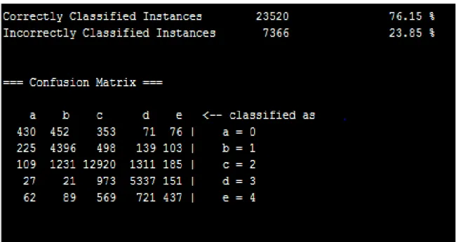
Confusion matrix will be generated after testing the model and this is the one that is mentioned below.
Confusion Matrix:
Figure 6: Confusion Matrix Result Table:
Table 1: Experimental results for Naive Bayes classifier
with_Unigrams with_Bigrams with_Stop wordswith_Stemmers Accuracy
No No No No 71.75
Yes No Yes No 72.59
Yes No Yes Yes 73.39
33
From this table, it can be observed that the accuracy is improving upon adding some features to the classifier. For this dataset, bigrams gave good result when compared to unigrams, as the reviewers usually express their opinion in two word combinations like 'very good', 'worth watching' and so on.
5.1.2 Random Forest using Scikit: Scikit:
Scikit is an API which offers machine learning libraries in Python for problems like classification, regression and clustering. This is open source and can be used for commercial purposes as well. SciPy, NumPy and matplotlib are the Python language extensions on which Scikit is built. NumPy is like a multi-dimensional array support for Python language.
Random Forest Classifier is imported from the module from sklearn.ensemble import RandomForestClassifier
After importing this classifier, the main steps to be performed are 1. Fitting the model with the training dataset
fit(X,y,sample_weight=None)
2. Predicting the labels for test dataset predict(X)
How the accuracy is determined:
After supplying the test set, to the model a result file will be generated. This result file consists of PhraseId's along with the predicted sentiment labels. The accuracy of this 'result file' should be determined now. This can be done by matching the PhraseId's and Sentiment labels of 'test file (consists of actual labels)' and 'result file (consists of predicted labels)'.
34
Here are the steps performed to complete this process:
1) Push the 'testfile(PhraseId SentenceId Phrase Sentiment)' into hdfs using -put command
hdfs -put absolute_path_of_testfile location_in_hdfs hdfs -put testfile /user/test1
2) Push the 'resultfile(PhraseId Sentiment)' into hdfs using -put command
3) Create two external tables in hive, one which points to 'testfile' in hdfs and the other which points to 'resultfile' which is also in hdfs.
4) Run an inner join query on the two tables based on the condition that the PhraseId's and Sentiment labels of both the tables match.
Here are the list of queries used for performing the above mentioned steps.
create external table actual_test(PhraseId string, SentenceId string, Phrase string, Sentiment string) row format delimited fields terminated by '\t' location '/user/test1';
create external table predicted_test(PhraseId string, Sentiment string) row format delimited fields terminated by ',' location '/user/test2';
select count(*) from (select a.PhraseId FROM actual_test a JOIN predcited_test b ON (a.PhraseId = b.PhraseId) where a.Sentiment=b.Sentiment) t;
35
Figure 7: Total number of matched instances
The total number of instances present in test file can be found with the help of query "select count(*) from actual_test"
36
The accuracy is calculated using predicted_instances / actual_instances = 24223/30886 = 78.42
Result Table:
Table 2: Experimental results for Random Forest classifier
Number of Trees (n)M Tries (m) Out of bag error Accuracy
100 118 26.31 77.80
150 118 25.11 78.39
200 118 23.59 78.42
250 118 23.03 78.55
From this table, it can be observed that the accuracy gets improved upon increasing the number of trees. But this improvement reaches a saturation point and doesn't increase further upon increasing the number of trees. The performance(running time) also gets degraded upon increasing the number of trees.
5.2 Multi tier results:
Some of the classifier models have been tried with multi tier architecture and the following sections are the results obtained from those models.
5.2.1 Stochastic Gradient Descent using Scikit: Evaluating the accuracy:
Same evaluation procedure has been followed, as is discussed under Random Forest Model.
37
Figure 9: Total number of matched instances
38 Accuracy = predicted_instances/actual_instances = 25388/30886
= 82.19%
Result Table:
Table 3: Experimental results for SGD classifier
SGD Model Accuracy
SGD 1 = Stopwords + Stemmers + N grams 79.42%
SGD 2 = SGD 1+ Grid Search 81.73%
SGD 3 = SGD 2+ POS Tagging 82.19%
From this table, it can be observed that Grid search along with parts of speech tagging worked the best. In Parts Of Speech(POS) tagging each feature(word) is tagged with its respective parts of speech and adjectives are mainly considered as they indicate some sentiment. In grid search different combinations of the given parameters will be applied and the best combination will be retained.
39
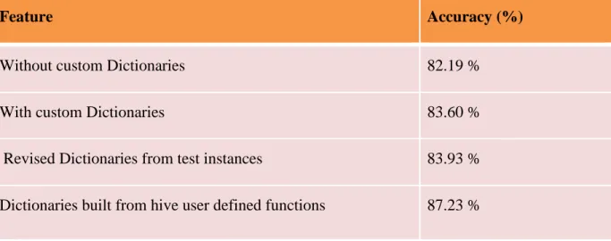
Table 4: Experiments with custom dictionaries for SGD classifier
These are the results obtained by using custom dictionaries. Revised dictionary results are obtained by considering the wrongly classified instances, extracting the important sentiment bearing words and then the dictionary is modified. In the next step, hive user defined table functions are used to further improve the dictionary.
Feature Accuracy (%)
Without custom Dictionaries 82.19 %
With custom Dictionaries 83.60 %
Revised Dictionaries from test instances 83.93 % Dictionaries built from hive user defined functions 87.23 %
40 CHAPTER 6
Conclusion and Future Work
This research paper proposes a new approach for dealing with multi class sentiment classification problems. Generally a classification model works better when the number of labels in the dataset are less in number, usually two or three. This paper proposes a classification model that deals with multiple labels. This model works in multiple phases and the sentiment of the data instance is fine-tuned in every phase. For instance, phase 1 classifies the data instance under three labels and the other phases further fine tunes the sentiment and predicts the final sentiment for the data instance. In this way, as the classification model works in multiple phases, the accuracy doesn't get degraded even when there are multiple labels.
Different classifiers like Naive Bayes, Random Forest and Stochastic Gradient Descent have been applied to this model to find the behavior of these classifiers on the dataset and the parameters that can be tuned for further improving the result. Application of various feature reduction techniques for this classification model, further improved the results and this has been discussed in the earlier sections.
The architecture proposed in this paper, the classifiers used for classifying this dataset and the various feature reduction techniques applied can be used for other text classification problems, which involve categorizing the data into multiple classes. Integrating various lexicons to this classification model, makes this model classify the data that consists of hierarchical classes.
This work can be used for other domains that involve classification problems by making some adjustments to the multi-tier predictive model and by using of various context specific lexicons.
41
LIST OF REFERENCES
[1] Liu, B., Blasch, E., Chen, Y., Shen, D. and Chen, G. (2013) ‘Scalable sentiment classification for Big Data analysis using Naïve Bayes Classifier’, IEEE International Conference on Big Data, 2013.
[2] Rachana Mishra., Ramjeevan Singh Thakur. (2014), 'An Efficient Approach for Supervised Learning Algorithms using Different Data Mining Tools for Spam Categorization', Fourth International Conference on Communication Systems and Network Technologies, 2014.
[3] Taifeng Wang., Jiang Bian., Shusen Liu., Yuyu Zhang., Tie-Yan Liu. (2013), ' Psychological Advertising: Exploring User Psychology for Click Prediction in Sponsored Search', 2013.
[4] Florian Heimerl, Steffen Lohmann, Simon Lange, Thomas Ertl. (2014), ' Word Cloud Explorer: Text Analytics based on Word Clouds', 47th Hawaii International Conference on System Science, 2014.
[5] Akaichi, J. (2013) ‘Social Networks’ Facebook' Statutes Updates Mining for Sentiment Classification’, International Conference on Social Computing, 2013. [6] Haruna Isah, Paul Trundle, Daniel Neagu, ' Social Media Analysis for Product
Safety using TextMining and Sentiment Analysis', 2011.
[7] Abdullah, S. S., Rahaman, M. S. and Rahman, M. S. (2013) ‘Analysis of stock market using text mining and natural language processing’, International Conference on Informatics, Electronics and Vision (ICIEV), 2013.
[8] Neethu, M. and Rajasree (2013) ‘Sentiment analysis in twitter using machine learning techniques’, Fourth International Conference on Computing, Communications and Networking Technologies (ICCCNT), 2013.
[9] Patel, B. and Shah, D. (2013) ‘Significance of stop word elimination in meta search engine’, International Conference on Intelligent Systems and Signal Processing (ISSP), 2013.
[10] Silva, C. and Ribeiro, B. (2003) ‘The importance of stop word removal on recall values in text categorization’, Proceedings of the International Joint Conference on Neural Networks, 2003.
42
[11] Harrag, F., El-Qawasmah, E. and Salman, A. M. S. Al- (2011) ‘Stemming as a feature reduction technique for Arabic Text Categorization’, 10th International Symposium on Programming and Systems, 2011.
[12] Warintarawej, P., Laurent, A., Pompidor, P. and Laurent, B. (2010)
‘Classification of brand names based on n-grams’, International Conference of Soft Computing and Pattern Recognition, 2010.
[13] Troussas, C., Virvou, M., Espinosa, K. J., Llaguno, K. and Caro, J. (2013)
‘Sentiment analysis of Facebook statuses using Naive Bayes classifier for language learning’, IISA 2013.
[14] Xue, D. and Li, F. (2015) ‘Research of Text Categorization Model based on Random Forests’, IEEE International Conference on Computational Intelligence & Communication Technology, 2015.
[15] Zhang, Y., Wang, C., Xiao, B. and Shi, C. (2012) ‘A New Method for Text Verification Based on Random Forests’, International Conference on Frontiers in Handwriting Recognition, 2012.
[16] Jain, T. I. and Nemade, D. (2010) ‘Recognizing Contextual Polarity in Phrase-Level Sentiment Analysis’, International Journal of Computer Applications, 7(5), pp. 12–21, 2010.
[17] Esmin, A. A. A., Roberto L. De Oliveira Jr. and Matwin, S. (2012) ‘Hierarchical Classification Approach to Emotion Recognition in Twitter’, 11th International Conference on Machine Learning and Applications, 2012.
[18] Li, J., Fong, S., Zhuang, Y. and Khoury, R. (2014) ‘Hierarchical Classification in Text Mining for Sentiment Analysis’, International Conference on Soft Computing and Machine Intelligence, 2014.
[19] Fan, N., Cai, W. and Zhao, Y. (2008) ‘Research on the Model of Multiple Levels for Determining Sentiment of Text’, IEEE Pacific-Asia Workshop on