A Comparison of Different Methods of Zero-Inflated Data Analysis and an Application in Health Surveys

Volume 16 | Issue 1 Article 29

5-1-2017

A Comparison of Different Methods of

Zero-Inflated Data Analysis and an Application in Health

Surveys

Si Yang

University of Rhode Island, yangsi06@gmail.com

Lisa L. Harlow

University of Rhode Island, lharlow@uri.edu

Gavino Puggioni

University of Rhode Island, gpuggioni@uri.edu

Colleen A. Redding

University of Rhode Island, credding@uri.edu

Follow this and additional works at:http://digitalcommons.wayne.edu/jmasm

Part of theApplied Statistics Commons,Social and Behavioral Sciences Commons, and the Statistical Theory Commons

This Regular Article is brought to you for free and open access by the Open Access Journals at DigitalCommons@WayneState. It has been accepted for inclusion in Journal of Modern Applied Statistical Methods by an authorized editor of DigitalCommons@WayneState.

Recommended Citation

Yang, S., Harlow, L. I., Puggioni, G., & Redding, C. A. (2017). A comparison of different methods of zero-inflated data analysis and an application in health surveys. Journal of Modern Applied Statistical Methods, 16(1), 518-543. doi: 10.22237/jmasm/1493598600

Cover Page Footnote

Si Yang is a Statistical Consultant and former Instructor at the University of Rhode Island. Email at yangsi06@gmail.com.

A Comparison of Different Methods of

Zero-Inflated Data Analysis and an Application in

Health Surveys

Si Yang

University of Rhode Island South Kingstown, RI

Gavino Puggioni

University of Rhode Island South Kingstown, RI

Lisa L. Harlow

University of Rhode Island South Kingstown, RI

Colleen A. Redding

University of Rhode Island South Kingstown, RI

The performance of several models under different conditions of zero-inflation and dispersion are evaluated. Results from simulated and real data showed that the zero-altered or zero-inflated negative binomial model were preferred over others (e.g., ordinary least-squares regression with log-transformed outcome, Poisson model) when data have excessive zeros and over-dispersion.

Keywords: zero-inflated analysis, count data

Introduction

In psychological, social, and public health related research, it is common that the outcomes of interest are relatively infrequent behaviors and phenomena. Data with abundant zeros are especially frequent in research studies when counting the occurrence of certain behavioral events, such as number of school absences, number of cigarettes smoked, number of hospitalizations, or number of unhealthy days. These types of data are called count data and their values are usually non-negative with a lower bound of zero and typically exhibit excessive zeros and over-dispersion (i.e., greater variability than expected).

Except for transforming the outcome to make it normal and using the general linear model, other alternative approaches can be taken in the context of a broader framework: generalized linear model (GLM). For example, the Poisson distribution becomes increasingly positively skewed as the mean of the response

variable decreases, which reflects a common property of count data (Karazsia and Van Dulmen, 2008). Thus, a typical way of analyzing count data includes specification of a Poisson distribution with a log link (the log of the expectation of a response variable is predicted by the linear combination of covariates, i.e., predictors) in a model known as Poisson regression.

Several other more rigorous approaches to analyzing count data include the zero-inflated Poisson (ZIP) model and the zero-altered Poisson model (ZAP, also called a hurdle model) that have been proposed recently to cope with an overabundance of zeros (Greene, 1994; King, 1989; Lambert, 1992; Mullahy, 1986). These two types of models both include a binomial process (modeling zeros versus non-zeros) and a count process. The difference between the two models is how they deal with different types of zeros: although the count process of ZAP is a zero-truncated Poisson (i.e. the distribution of the response variable cannot have a value of zero), the count process of ZIP can produce zeros (Zuur, et al., 2009). One of the assumptions of using Poisson regression is that the mean and variance of a response variable are equal. In reality, it is often the case that the variance is much larger than the mean. Variations of negative binomial (NB) models can be used when over-dispersion exists even in the non-zero part of the distribution. Although a Poisson distribution contains only a mean parameter (μ), a negative binomial distribution has an additional dispersion parameter (k) to capture the amount of over-dispersion. Thus, the zero-inflated negative binomial (ZINB) model and zero-altered negative binomial (ZANB) model were introduced to deal with both zero-inflation and over-dispersion.

Traditionally, dichotomizing or transforming the dependent variables have been used as solutions to handle the non-normality of the data. Approaches such as a Poisson model, NB model, ZIP/ZAP models, or ZINB/ZANB models have recently been demonstrated and compared to analyze zero-inflated count data through several tutorial style papers (e.g., Atkins, 2012; Karazsia and Van Dulmen, 2008; Loeys, et al., 2012; Vives, et al., 2006). Each of these papers largely focus on a single empirical study and models were only being compared in one condition. The current study focused on comparing a set of models under different conditions of zero-inflation and skewness and aimed to offer clear guidelines as to which model to use under a certain condition.

GLM and Poisson regression

The GLM is a flexible modeling framework that allows the response variables to have a distribution form other than normal. It also allows the linear model of

several covariates to be related to a response variable via arbitrary choices of link functions. Zuur et al. (2009) summarized that building a GLM consists of three steps: a) choosing a distribution for the response variable (Y); b) specifying covariates (X); and c) choosing a link function between the mean of the response variable (E(Y)) and a linear combination of the covariates (βX). Classical models such as analysis of variance (ANOVA) and ordinary least squares regression also belong to the GLM when Y is normally distributed. Y can also be specified as other distributional forms in the exponential family such as a binomial distribution, Poisson distribution, negative-binomial distribution, and gamma distribution. The link function brings together the expectation of the response variable and the linear combination of the covariates. For ordinary least-squares regression, the function to estimate the expected value of Y is βX = E(Y); it is termed as an identity link. Specifying a logit link as βX = log(E(Y) / (1−E(Y))) is usually used for logistic regression to predict the expectation of a binary response variable. The probability mass function (p.m.f) of a Poisson distribution is a s follows:

Pr

(

)

-m

_m

y_i! ,yi =0,1,2,...

where μ is the count mean. Let X = (X1, …, Xp) be a vector of covariates and

β = (β1, …, βp) be a vector of regression parameters. The logarithm of μ is

assumed to be a linear combination of p covariates of the form E Y

(

)

m

( )

b

The conditional mean and conditional variance are equal for the Poisson regression model, that is E(Y|X) = Var(Y|X) = μ. The greater the mean the greater is the variability of the data. A large proportion of zeros in the count data leads to a smaller mean value than that of the variance.

Negative binomial regression model

The assumption that the variance of counts is equal to the mean also implies that the variability of the outcomes sharing the same covariates values (a population has the same values for X1, X2, … , Xp) is equal to the mean. If it fails to be true,

the estimates of the regression coefficients can still be consistent using Poisson regression, but the standard errors can be biased. They usually tend to be too

small and thus increase the rate of Type I error (false positive results) (Hilbe, 2014). When analyzing data to explore relationships between variables or make predictions, we would not expect we have measured every variable that contributes to the rates of the outcome events. There will always be residual variation in the response variables. For instance, Roebuck et al. (2004) studied how adolescent marijuana use might relate to school attendance (estimated by number of days truant) by analyzing data from the National Household Survey on Drug Abuse. It is unlikely that adolescent marijuana users will have the same rate of being truant; specifically, there is more variation in school attendance among marijuana users. To account for greater variation, the negative binomial model has been proposed as a generalization of the Poisson model. The negative binomial distribution has the following form:

Pr

(

)

(

)

( )

m

m

m

where μ is the mean and k is the dispersion parameter. The variance of the above distribution is μ + μ2_{/k, and hence decreasing values of k correspond to} increasing levels of dispersion. As k increases towards positive infinity, a Poisson distribution is obtained. The negative binomial regression model is able to capture the over-dispersion in count data that the simple Poisson model cannot. However, the problem of excessive zeros is still not solved, as researchers may be interested in finding the special meaning underlying the zero-inflation.

Zero-inflated regression models

Lambert (1992) proposed an approach to model zero-inflation in count data in what is referred to as a ZIP model. In this model, two kinds of zeros are thought to exist in the data: structural zeros (or true zeros) from a non-susceptible group (i.e., those that do not have the attribute or experience of interest, such as healthy people without a disease) and random zeros (or false zeros) for those from a susceptible group (e.g., those that have a disease in a health-based study who may falsely indicate a score of zero). The probability of being in a susceptible group can be estimated by information from covariates with a logistic link. If an individual is from the susceptible group, his or her count is a random variable from a Poisson distribution with mean µ. The marginal distribution of the ZIP model is as follows:

Pr

(

)

p

( )

p

p

m

The Poisson hurdle model (i.e., ZAP) as an alternative was introduced by Mullahy (1986) and modified by King (1989). It models all zeros as one part and a zero-truncated part for all non-zero observations. The main difference with ZIP is that hurdle models don’t distinguish true and false zeros and all zero observations are thought to come from a non-susceptible group:

Pr

(

)

p

p

m

(

)

Because a Poisson distribution assumes that the variance of the outcome variable equals its mean, when over-dispersion also comes from the non-zero part (i.e., the variance is much bigger than the mean even for the non-zero part), both ZIP and ZAP models can be extended to ZINB or ZANB models to deal with zero-inflation and over-dispersion at the same time. These types of models have become popular recently and have been used to analyze number of cigarettes smoked per day (Schunck & Rogge, 2012), dental health status (Wong & Lam, 2012), depressive symptoms (Beydoun, et al., 2012), and alcohol consumption (Atkins, 2012), etc. The major advantage of using models specially dealing with zero-inflation is that they not only reduce biases resulting from the extreme non-normality but also have the ability to model the effect on subjects’ susceptibility and magnitude at the same time.

Proposed Study

For count data, depending on an outcome’s mean-variance relationship and proportion of zeros, the choices for modeling its distribution range from standard Poisson and negative binomial to ZIP, and ZINB (or ZAP and ZANB). However, some researchers argue that they have seen cases where ZIP models were inadequate and ZINB also couldn’t be reasonably fitted to the data (Famoye & Singh, 2006). Warton (2005) also criticized such zero-inflated models as being too routinely applied, leading to overuse. He analyzed 20 multivariate abundance

datasets extracted from the ecology literature using three different approaches: least squares regression on transformed data, log-linear models (Poisson and negative binomial regression), and zero-inflated models (ZIP and ZINB), and then compared each model’s goodness-of-fit. The result showed that a Gaussian (i.e., normally distributed) model (e.g., least squares regression) based on a transformed outcome fit the data surprisingly better than fitting zero-inflated count distributions. This study also suggested that negative binomial regression had the best fit, and that special techniques for dealing with excessive zeros may be unnecessary.

Based on these open questions in the field, there appears to be a conflict since there is increasing popularity of zero-inflated models, although some empirical evidence has tended to show no better fit for these models compared with the traditional least squares method conducted on transformed data. Moreover, there is much disagreement about which zero-inflated model to choose from among ZIP, ZINB, ZAP, and ZANB. In the zero-inflation data analysis literature, proposing an extensional zero-inflated model or comparing different models are often motivated and illustrated by a single empirical study. These can look more like case studies in which each dataset or applied situation has its particular uniqueness. It is possible that the discrepancy in the results from these studies depends on having a different proportion of zeros and different skewness in the non-zero part. It is becoming apparent that having data with excessive zeros is the norm in many situations, with or without known reasons. However, it is not clear what the proportion of zeros is, after which the data should be considered as zero-inflated, and what the underlying mechanism of abundant zeros is. Further, when researchers have collected data with abundant zeros, should zero-inflated models be used, and if so, which one should be used? These are questions that have unclear or controversial answers in the zero-inflation literature, and which are driving the proposed research. This study used systematic methods to try to answer these questions.

Another consideration is that, a full range of these methods hasn’t been compared and tested under different conditions. The purpose of this study was to examine the performance of different techniques dealing with zero-inflation. Both simulated data and empirical data with and without known reasons for zero-inflation were analyzed. Specifically, this study addressed the following research questions:

1. Under conditions of different degrees of zero-inflation (i.e. proportion of zeros in the response variable) but the same level of dispersion,

which of the following models is superior: a) least squares regression with a transformed outcome; b) Poisson regression; c) negative binomial regression; d) ZIP; e) ZINB; f) ZAP; or g) ZANB?

2. Under conditions of different degrees of dispersion but the same zero-inflation level, which of the following models is superior: a) least squares regression with a transformed outcome; b) Poisson regression; c) negative binomial regression; d) ZIP; e) ZINB; f) ZAP; or g) ZANB?

3. Finally, for the empirical data from a national health survey with a zero-inflated and over-dispersed response variable, which of the following models is superior: a) least squares regression with a transformed outcome; b) Poisson regression; c) negative binomial regression; d) ZIP; e) ZINB; f) ZAP; or g) ZANB?

Methods

Simulation Study Design Data were generated with a mix of zeros and a negative binomial distribution. A brief literature review on the frequency of various health survey outcomes showed that the percentage of zeros tends to range from 20% to 90% (Beydoun, et al., 2012; Lin & Tsai, 2012; Mahalik, et al., 2013); thus, four conditions with varying probability of zeros (w in Table 1) for the response variable were tested in the current study to reflect this range. A condition of no zero-inflation (w = 0.00) was also tested as a baseline comparison. In order to examine the effect of over-dispersion in the non-zero part, a dispersion parameter k with the following values: 1, 5, 10, and 50 were pre-specified. These values represent a reasonable range of dispersion to help assess the merit of various models with varying distributions. The bigger the k the less dispersed the variable is and it approaches a Poisson distribution when k > 10µ (Bolker, 2008). The response variable was generated with a negative binomial distribution with a different proportion of zeros added. The simulation study was a 5 (i.e., Factor A: degree of zero-inflation) x 4 (i.e., Factor B: degree of dispersion) factorial design that was examined for the 7 models listed for Factor C, as shown in Table 1.

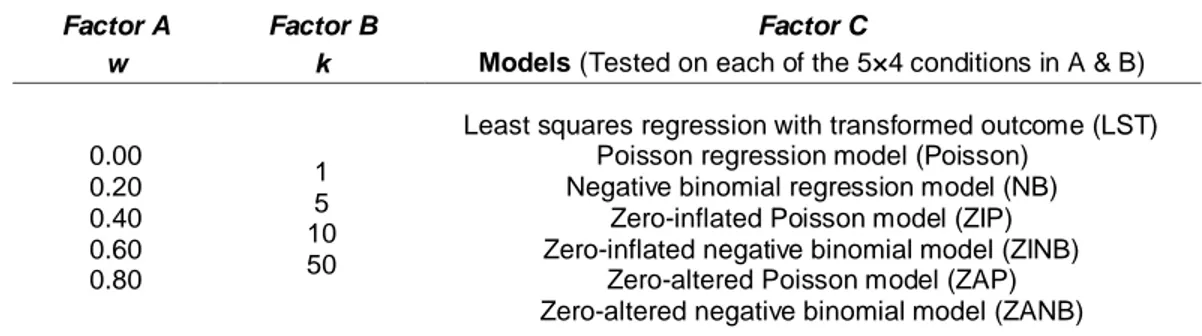
Table 1. Simulation design factors

Factor A Factor B Factor C

w k Models (Tested on each of the 5×4 conditions in A & B)

0.00 0.20 0.40 0.60 0.80 1 5 10 50

Least squares regression with transformed outcome (LST) Poisson regression model (Poisson)

Negative binomial regression model (NB) Zero-inflated Poisson model (ZIP) Zero-inflated negative binomial model (ZINB)

Zero-altered Poisson model (ZAP) Zero-altered negative binomial model (ZANB)

Note. Factor A indicates the proportion of zeros in the simulated data, ranging from w = 0 (i.e., none) to .80 (i.e.,

high). Factor B indicates the degree of dispersion in the data, ranging from k = 1 (i.e., high) to 50 (i.e., low).

Generating Simulated Datasets To provide a reasonable prediction model to explore in this study, a count response variable Y and two different kinds of covariates, X1 and X2, were simulated. X1 was assumed to be a binary variable whose values were 0 or 1 with Pr(X1 = 0) = Pr(X1 = 1) = 0.5. X2 was set to follow a standard normal distribution, N(0,1). Regression coefficients β1 and β2 for the two covariates were set to be 0.3 and 0.5 for the population model to allow for a medium and large value, respectively. It is recognized that the two values cannot be seen as standardized effect sizes as the scores for Y and X1 are not standardized. However, regression coefficients of 0.3 and 0.5 can be seen as reasonable choices that allow for a comparison between different levels of prediction for the two covariates. To ensure accurate results, 2000 replications (i.e., simulation size, S = 2000), each with sample size n = 500, were generated. The simulated mean for the count process (µ) was 1.33 (SD = 0.03) across all simulations. The decisions on the number of simulations and sample size were made by referring to previous simulation studies on zero-inflated data (e.g., Lambert, 1992; Min & Agresti, 2005; Williamson, et al., 2007).

Model Selection Criteria The model with minimum AIC (Akaike information criterion) was considered as the best model to fit the data (Bozdogan, 2000). AIC is given by:

AIC = −2logL(θ) + 2c,

where L(θ) is the maximized likelihood function for the estimated model and −L(θ) offers summary information on how much discrepancy exists between the model and the data, where c is the number of free parameters in the model.

AIC assesses both the goodness of fit of the model and the complexity of the model. It rewards the model fit by the maximized log likelihood term 2logL(θ), and also prefers a relatively parsimonious model by having c as a measure of complexity. There are two challenges for calculating a comparable AIC for the LST model. First, AIC can only be used to compare models with the exact same response variable. Second, a response variable in the LST model is assumed to be continuous, whereas in other models it is a count. It is not correct to compare the log-likelihood of discrete distribution models and continuous distribution models, as the former is the sum of the log probabilities and the latter is the sum of the log densities. Warton (2005) used a discretization method to address the issue and we applied the same approximation approach in this paper. For the LST model, the Gaussian distribution for AIC calculation was discretized as below.

L

( )

q

(

_{m, ˆ}

_s

)

(

)

m

s

(

)

m

s

å

where

m

ˆ

_ˆ

s

Empirical Data Analysis

Analyses were conducted on an existing data set to further assess different procedures. The Behavioral Risk Factor Surveillance System (BRFSS) collected information on health risk behaviors, health conditions, health care access, and use of preventive services (CDC, 2012). In this portion of the study based on actual data, the relationship between physical activity and health related quality of life was examined after controlling for age and gender, continuous and binary covariates, respectively.

Participants The data were obtained from the 2011 Rhode Island BRFSS, a random-digit telephone health survey of adults 18 years of age or older. Of 6533 participants involved in the survey, 38.3% were males and 61.7% were females ranging in age from 18 to 98 (M = 55.51, SD = 16.90).

Measures

Health Related Quality of Life (HRQoL): The overall number of mentally or physically unhealthy days (UNHLTH) in the last 30 days was used as an indicator of having poor HRQoL. The summary index of unhealthy days was calculated by combining the following two questions (CDC, 2012), with a logical maximum of 30 unhealthy days:

1. “Now thinking about your physical health, which includes physical illness and injury, for how many days during the past 30 days was your physical health not good?”

2. “Now thinking about your mental health, which includes stress, depression, and problems with emotions, for how many days during the past 30 days was your mental health not good?”

Physical Activity (PA): A set of questions in the BRFSS captured data on three key domains of physical activity: leisure-time, domestic, and transportation. A summary score for physical activity was calculated and then was categorized into four levels according to CDC’s 2008 Physical Activity Guidelines for Americans, a) highly active, b) active, c) insufficiently active, and d) inactive, with higher scores indicating higher levels of physical activity.

Analysis Participants reporting 30 physically or mentally unhealthy days during the past month were not included in the analysis. These individuals were considered as patients with long-term sickness who did not meet the inclusion criteria for this study. PA, age, gender, and their interactions with PA were entered as predictors of having poor HRQoL. Seven regression models described above were used to fit the data. In addition to using AIC values to evaluate the models, Vuong’s tests were also used for model comparisons. Vuong’s test is likelihood-ratio based for comparing nested, non-nested, or overlapping models in a hypothesis testing framework (Vuong, 1989). The null hypothesis was that both models were equally close to the true model. To control for Type I error rate for the several model comparisons that were made, p < .01 was used as a criterion for a statistically significant result.

Statistical Program R (R Core Team, 2013) was used for both data simulation and data analyses. Function rnbinom() was used to generate random negative binomial variables. Functions hurdle() and zeroinfl() from package

pscl (Jackman, 2008) were used to fit data with zero-altered and zero-inflated models; and glm() from package stats was used to fit LST, Poisson, and NB models.

Results

Results from simulation study

Average AIC values and selection rates (i.e., percentages of runs having the lowest AIC, which indicated a more preferred model) across all simulations for the five levels of zero-inflation combined with four levels of over-dispersion on the seven models are presented in Table 2.

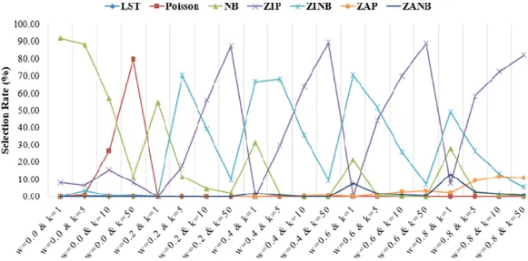
Figure 1 gives a visual presentation of how selection rates changed across different conditions for different models. Under the no zero-inflation condition (w = 0.0), a Poisson model was more preferred when k = 50 (i.e., low dispersion) and a NB model was more preferred when k = 1, 5, or 10 (i.e., high to moderate dispersion). When data did exhibit zero-inflation, even with just 20% of zeros, a ZIP model was more preferred with low dispersion (k = 10 or 50); a ZINB model was more preferred with high dispersion (k = 1 or 5); the Poisson model and the LST model yielded much larger average AIC values with a 0% selection rate; and the NB model had higher selection rates as k and w got smaller (i.e., high dispersion and low proportion of zeros). The ZIP, ZINB, ZAP, and ZANB had similar AIC values across all of the conditions, however, ZIP and ZINB had much higher percentages of being more preferred models compared with ZAP and ZANB.

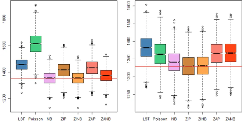
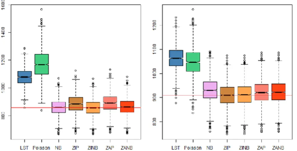
Boxplots for the AIC values across different conditions were constructed for the seven models. Figures 2.1 and 2.5 show the most (k = 1) and least (k = 50) over-dispersed levels of the five conditions of proportion of zeros (i.e., w = 0.0, 0.2, 0.4, 0.6, and 0.8). For each figure, the left side pertains to k = 1 and the right side to k = 50. Further, a reference line was added to all figures by using the minimum mean AIC values. For definitions of the seven models, refer to the note in Figure 1.

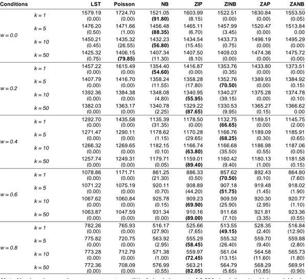
Table 2. Mean AIC values, and percentage with the lowest AIC across all simulations (in parenthesis), for 12 conditions on 7 models

Conditions LST Poisson NB ZIP ZINB ZAP ZANB

w = 0.0 k = 1 1579.19 1724.70 1521.05 1603.99 1522.51 1630.84 1553.50 (0.00) (0.00) (91.80) (8.15) (0.00) (0.00) (0.05) k = 5 1476.20 1471.66 1456.48 1465.11 1457.99 1520.47 1513.84 (0.50) (1.00) (88.35) (6.70) (3.45) (0.00) 0.00 k = 10 1450.21 1435.32 1432.23 1434.54 1433.73 1496.19 1495.29 (0.45) (26.55) (56.80) (15.45) (0.75) (0.00) (0.00) k = 50 1425.32 1406.15 1407.34 1407.50 1409.03 1474.36 1475.72 (0.75) (79.85) (11.30) (8.10) (0.00) (0.00) (0.00) w = 0.2 k = 1 1457.22 1615.49 1354.40 1416.87 1353.76 1433.80 1373.51 (0.00) (0.00) (54.60) (0.00) (0.35) (0.00) (0.00) k = 5 1407.79 1416.70 1358.24 1358.28 1352.76 1389.93 1384.92 (0.00) (0.00) (11.55) (17.80) (70.50) (0.00) (0.15) k = 10 1392.36 1384.38 1348.08 1340.95 1340.27 1375.28 1374.78 (0.00) (0.00) (4.80) (55.95) (39.15) (0.00) (0.10) k = 50 1382.03 1363.17 1340.78 1329.22 1330.53 1365.27 1366.62 (0.00) (0.00) (2.25) (87.65) (9.95) (0.15) 0.00 w = 0.4 k = 1 1292.70 1435.58 1135.39 1178.50 1132.75 1189.51 1145.75 (0.00) (0.00) (31.35) (0.00) (66.65) (0.00) (2.00) k = 5 1271.47 1290.11 1178.62 1170.28 1166.76 1189.09 1185.91 (0.00) (0.00) (1.15) (29.65) (68.25) (0.30) (0.65) k = 10 1266.32 1269.65 1182.15 1166.74 1166.68 1186.98 1187.06 (0.00) (0.00) (0.10) (63.80) (35.50) (0.55) (0.05) k = 50 1257.74 1249.31 1179.71 1159.01 1160.42 1180.13 1181.58 (0.00) (0.00) (0.05) (89.40) (9.40) (1.00) (0.15) w = 0.6 k = 1 1078.86 1171.71 861.25 886.33 857.62 892.43 864.80 (0.00) (0.00) (21.30) (0.50) (70.50) (0.10) (7.60) k = 5 1071.22 1075.19 920.11 908.89 907.18 919.48 918.02 (0.00) (0.00) (0.70) (44.20) (51.75) (1.45) (1.90) k = 10 1067.62 1060.84 925.78 909.23 909.59 920.30 920.77 (0.00) (0.00) (0.15) (69.90) (25.90) (2.95) (1.10) k = 50 1063.87 1047.59 931.34 910.16 911.68 921.81 923.36 (0.00) (0.00) (0.00) (89.00) (7.10) (3.35) (0.55) w = 0.8 k = 1 782.26 765.93 516.17 525.66 513.55 528.35 516.84 (0.00) (0.00) (27.90) (7.65) (49.15) (2.40) (12.90) k = 5 775.82 720.75 563.92 555.29 555.32 559.70 559.88 (0.00) (0.00) (2.95) (58.45) (26.40) (9.40) (2.80) k = 10 773.28 712.79 571.38 559.97 561.04 564.58 565.73 (0.00) (0.00) (1.00) (72.45) (13.15) (11.60) (1.80) k = 50 772.36 708.09 576.99 563.21 564.79 568.29 569.91 (0.00) (0.00) (0.55) (82.05) (5.65) (10.85) (0.90)

Note: Numbers in parentheses are percentages (%) of simulations out of 2,000 simulations in which model had

the lowest AIC value (most preferred); w is the proportion of zeros and k is the dispersion parameter used to

simulate the data. LST = least squares regression with transformed outcome, Poisson = Poisson regression model, NB = negative binomial regression model, ZIP = zero-inflated Poisson model, ZINB = zero-inflated negative binomial model, ZAP = zero-altered Poisson model, ZANB = zero-altered negative binomial model.

Note: w is the proportion of zeros and k is the dispersion parameter used to simulate the data. LST = least squares regression with transformed outcome, Poisson = Poisson regression model, NB = negative binomial regression model, ZIP = zero-inflated Poisson model, ZINB = zero-inflated negative binomial model, ZAP = zero-altered Poisson model, ZANB = zero-altered negative binomial model.

Figure 1. Percentages of having the lowest AIC across 2000 simulations

Figure 2.2. Boxplot of AIC from seven models (w = 0.2)

Figure 2.4. Boxplot of AIC from seven models (w = 0.6)

Figure 2.5. Boxplot of AIC from seven models (w = 0.8)

From the boxplots, we can see that when k = 1, the NB model and the ZINB model had much lower AIC values compared with the Poisson and the ZIP model. The difference in AIC values between zero-inflated models (i.e., ZIP and ZINB) and zero-altered models (i.e., ZAP and ZANB) showed a tendency to get smaller as there was an increase of zero-inflation and dispersion. AIC values for the ZINB model were always low across all conditions.

Results from empirical data analysis

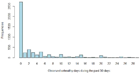
Descriptive statistics such as means (and standard deviations) or frequencies (and percentages) for the variables of age, sex, UNHLTH and physical activity are presented in Table 3. Participants reported an average of 3.63 unhealthy days during the past 30 days with a variance of 36.84, which was much larger than the mean; and 44.67% of the participants reported 0 unhealthy days.

Table 3. Descriptive statistics for independent and dependent variables (n = 5670)

Variable Mean SD Frequency (%)

Age (years) 55.03 16.87 Sex Male 2126 38.7 Female 3362 61.3 # Unhealthy Days 3.63 6.07 Physical Activity Highly Active 1659 32.5 Active 1059 20.8 Insufficiently Active 1059 20.8 Inactive 1323 25.9

Figure 3 presents the frequency plot of the response variable, UNHLTH. Notice that this variable showed an extremely right skewed distribution with a spike at zero.

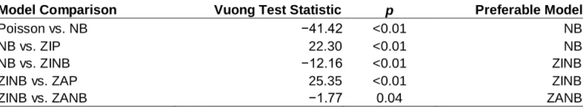
Seven models described above were used to fit the data. AIC values and −2log-likelihood for each model are presented in Table 4.1. The Poisson regression model had the largest AIC values, demonstrating a poor fit to the data. Of the remaining six models, the NB, ZINB, and ZANB models had smaller AICs compared with the ZIP, ZAP, and LST models, indicating better fit with the data for the three negative binomial based models. ZINB and ZANB models yielded similar AICs and are considered as the best models even after penalizing the number of parameters in the model. Since not all of the models were nested with each other, under the null hypothesis that the models were indistinguishable, Vuong tests were used to further compare the above models. LST couldn’t be compared because it has a different term for its dependent variable, i.e. it is log-transformed. The first comparison was made between the Poisson model and the NB model, with a Vuong test statistic of −42.41, and p < 0.01, indicating the NB model was more preferred. The more preferable model was then compared with the next model. After a series of tests and model comparisons (as shown in Table 4.2), ZANB was chosen as the best model. ZINB could be viewed as a second choice with a Vuong test statistic of −1.77, and p = 0.04 compared to ZANB, although the p-value was not within the range needed to control Type I error rate.

Table 4.1. Model fit comparison for the BRFSS data

LST Poisson NB ZIP ZINB ZAP ZANB

AIC 24050.78 47932.45 21447.22 27814.26 21060.95 27814.26 21060.06 −2log-likelihood 24046.78 47908.45 21421.22 27766.26 21010.95 27766.26 21010.06

c 13 12 13 24 25 24 25

Note: AIC = the Akaike Information Criterion, and c is the number of free parameters in the model. LST = least squares regression with transformed outcome, Poisson = Poisson regression model, NB = negative binomial regression model, ZIP = zero-inflated Poisson model, ZINB = zero-inflated negative binomial model, ZAP = zero-altered Poisson model, ZANB = zero-altered negative binomial model.

Table 4.2. Vuong non-nested tests results for the BRFSS data

Model Comparison Vuong Test Statistic p Preferable Model

Poisson vs. NB −41.42 <0.01 NB

NB vs. ZIP 22.30 <0.01 NB

NB vs. ZINB −12.16 <0.01 ZINB

ZINB vs. ZAP 25.35 <0.01 ZINB

ZINB vs. ZANB −1.77 0.04 ZANB

Note: Poisson = Poisson regression model, NB = negative binomial regression model, ZIP = zero -inflated Poisson model, ZINB = zero-inflated negative binomial model, ZAP = zero-altered Poisson model, ZANB = zero-altered negative binomial model.

Table 5.1. Estimated regression coefficients (and standard errors) for LST, Poisson, and NB Regressor LST SE Poisson SE NB SE Intercept 0.713*** (0.040) 0.987*** (0.023) 0.983*** (0.080) PA_active 0.032 (0.068) 0.097* (0.038) 0.116 (0.134) PA_insufficiently active −0.004 (0.068) 0.021 (0.039) 0.027 (0.133) PA_inactive 0.162** (0.062) 0.360*** (0.033) 0.365** (0.122) SEX_female 0.117** (0.053) 0.173*** (0.029) 0.178 (0.104) AGE −0.007*** (0.002) −0.010*** 0.000 −0.010** (0.003) PA_active*SEX_female 0.049 (0.086) −0.002 (0.046) −0.025 (0.169) PA_insufficiently active*SEX_female 0.158 (0.085) 0.231*** (0.046) 0.225 (0.168) PA_inactive*SEX_female 0.11 (0.080) 0.089* (0.040) 0.083 (0.157) PA_active*AGE 0.001 (0.003) 0.004** (0.001) 0.005 (0.005) PA_insufficiently active*AGE 0.005 (0.003) 0.009*** (0.001) 0.009 (0.005) PA_inactive*AGE 0.007** (0.002) 0.012*** (0.001) 0.012** (0.005)

Note: “Male” was the reference group for sex and “highly active” was the reference group for physical activity. LST = least squares regression with transformed outcome, Poisson = Poisson regression model, NB = negative binomial regression model.

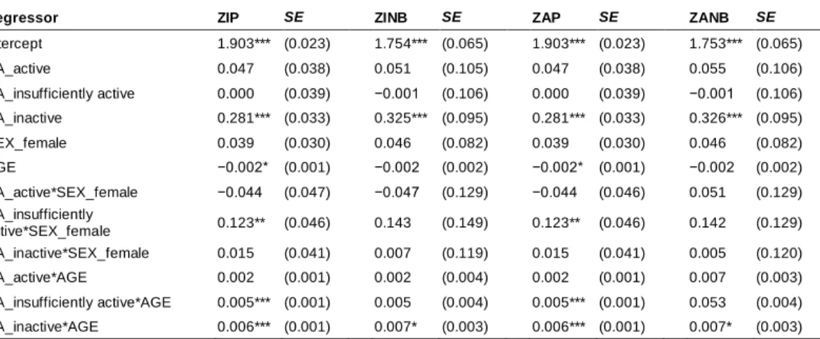
Table 5.2. Estimated regression coefficients (and standard errors) for ZIP, ZINB, ZAP, and ZANB under the Count Model

Regressor ZIP SE ZINB SE ZAP SE ZANB SE

Intercept 1.903*** (0.023) 1.754*** (0.065) 1.903*** (0.023) 1.753*** (0.065) PA_active 0.047 (0.038) 0.051 (0.105) 0.047 (0.038) 0.055 (0.106) PA_insufficiently active 0.000 (0.039) −0.001 (0.106) 0.000 (0.039) −0.001 (0.106) PA_inactive 0.281*** (0.033) 0.325*** (0.095) 0.281*** (0.033) 0.326*** (0.095) SEX_female 0.039 (0.030) 0.046 (0.082) 0.039 (0.030) 0.046 (0.082) AGE −0.002* (0.001) −0.002 (0.002) −0.002* (0.001) −0.002 (0.002) PA_active*SEX_female −0.044 (0.047) −0.047 (0.129) −0.044 (0.046) 0.051 (0.129) PA_insufficiently active*SEX_female 0.123** (0.046) 0.143 (0.149) 0.123** (0.046) 0.142 (0.129) PA_inactive*SEX_female 0.015 (0.041) 0.007 (0.119) 0.015 (0.041) 0.005 (0.120) PA_active*AGE 0.002 (0.001) 0.002 (0.004) 0.002 (0.001) 0.007 (0.003) PA_insufficiently active*AGE 0.005*** (0.001) 0.005 (0.004) 0.005*** (0.001) 0.053 (0.004) PA_inactive*AGE 0.006*** (0.001) 0.007* (0.003) 0.006*** (0.001) 0.007* (0.003)

Note: “Male” was the reference group for sex and “highly active” was the reference group for physical activity.

For zero-inflated and zero-altered models, Count Model has relationship between covariates and count mean and Zero-inflation Model has relationship between covariates and probability of zeros. ZIP = zero-inflated Poisson model, ZINB = zero-inflated negative binomial model, ZAP = zero-altered Poisson model, ZANB = zero-altered negative binomial model. Significance levels: *** = 0.001, ** = 0.01, * = 0.05.

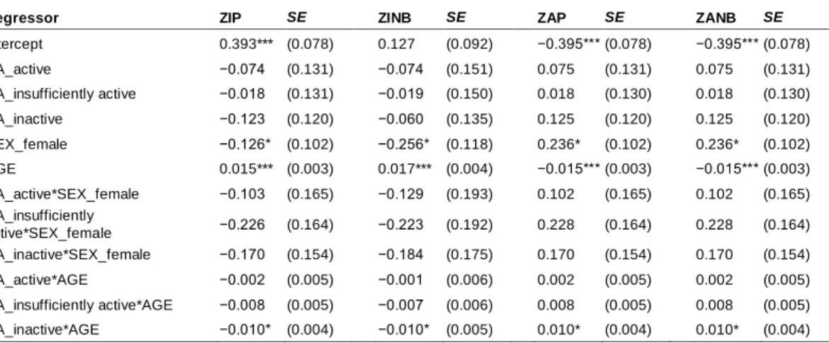
Table 5.3. Estimated regression coefficients (and standard errors) for ZIP, ZINB, ZAP, and ZANB under the Zero-Inflation Model

Regressor ZIP SE ZINB SE ZAP SE ZANB SE

Intercept 0.393*** (0.078) 0.127 (0.092) −0.395*** (0.078) −0.395*** (0.078) PA_active −0.074 (0.131) −0.074 (0.151) 0.075 (0.131) 0.075 (0.131) PA_insufficiently active −0.018 (0.131) −0.019 (0.150) 0.018 (0.130) 0.018 (0.130) PA_inactive −0.123 (0.120) −0.060 (0.135) 0.125 (0.120) 0.125 (0.120) SEX_female −0.126* (0.102) −0.256* (0.118) 0.236* (0.102) 0.236* (0.102) AGE 0.015*** (0.003) 0.017*** (0.004) −0.015*** (0.003) −0.015*** (0.003) PA_active*SEX_female −0.103 (0.165) −0.129 (0.193) 0.102 (0.165) 0.102 (0.165) PA_insufficiently active*SEX_female −0.226 (0.164) −0.223 (0.192) 0.228 (0.164) 0.228 (0.164) PA_inactive*SEX_female −0.170 (0.154) −0.184 (0.175) 0.170 (0.154) 0.170 (0.154) PA_active*AGE −0.002 (0.005) −0.001 (0.006) 0.002 (0.005) 0.002 (0.005) PA_insufficiently active*AGE −0.008 (0.005) −0.007 (0.006) 0.008 (0.005) 0.008 (0.005) PA_inactive*AGE −0.010* (0.004) −0.010* (0.005) 0.010* (0.004) 0.010* (0.004)

Note: “Male” was the reference group for sex and “highly active” was the reference group for physical activity. For zero-inflated and zero-altered models, Count Model has relationship between covariates and count mean and Zero-inflation Model has relationship between covariates and probability of zeros. ZIP = zero-inflated Poisson model, ZINB = zero-inflated negative binomial model, ZAP = zero-altered Poisson model, ZANB = zero-altered negative binomial model. Significance levels: *** = 0.001, ** = 0.01, * = 0.05.

Regression coefficients and standard errors were estimated and presented in

Table 5.1 and 5.2 for each of the seven models when applied to the BRFSS dataset. Standard errors estimated from different models were quite different. There was a tendency for the worse models to have smaller standard errors. For instance, although estimates from the Poisson model were similar to those from the NB model, their standard errors were much smaller, thus yielding significant results for most of the regressors, which was most likely not accurate. It was the same when comparing ZIP versus ZINB and ZAP versus ZANB.

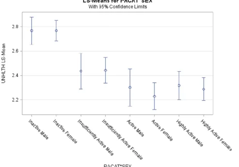
With PA (i.e., physical activity), gender, age, PA*gender, and PA*age predicting both the count model and zero-inflation model, Table 5.2 shows parameter estimates from the ZANB model (the final model). Participants in the highly active group and males were used as reference groups. After controlling for age, gender, and their interaction terms with PA, compared with highly active people, inactive people were likely to experience 1.39 (= exp(0.326), p < 0.001) more unhealthy days. This trend can also be seen in Figure 4, where both inactive males and females had higher means of UNHLTH than other groups of participants. (Male) gender (odds ratio = 1.27, p < 0.05) and younger age (odds ratio = 0.99, p < 0.001) were the only results to be significant predictors for those who experienced 0 unhealthy days versus those who experienced more than 0 unhealthy days. Thus, females and older people were more likely to report

unhealthy days, although it should be pointed out that the odds ratio for age was not very meaningful in size, even if significant.

Figure 4. Least-squared Means of UNHLTH by PA and Gender with 95% Confidence Limits

Discussion

This study evaluated seven regression models under various conditions of zero-inflation and dispersion by analyzing simulated datasets and an empirical dataset. Results from both studies suggested that when the data include excessive zeros (even as low as 20%) and over-dispersion, zero inflated models (i.e. ZIP, ZINB, ZAP, and ZANB) perform better than Poisson regression and ordinary least-squares regression with transformed outcomes (LST). It was only when fitting data with no zero-inflation and the least dispersion (i.e., w = 0.0 and k = 50) in the simulation study, that the Poisson regression model performed well and had the highest selection rate.

The poor fit from the LST might be that the log-transformation still fails to correct the non-normality and to address the inflation of zeros. Another drawback

of using a transformation is that the regression coefficients are harder to interpret. The Poisson distribution is the probability model usually assumed for count data, however, zero-inflated count data usually tend to have much bigger variance than the mean, which violates its assumption that the mean equals the variance. In both cases, when failing to address the problem of zero-inflation and over-dispersion, standard errors of the estimates tended to be deflated or under estimated (Hilbe, 2014). Furthermore, if inappropriately choosing the LST or the Poisson model, there is greater tendency to make Type I errors, i.e. a variable may appear to be a significant predictor when it is in fact, not significant. Estimated regression coefficients from Table 5.1 demonstrate this kind of bias.

Results from these studies of simulated and real data support using special zero inflated models for zero-inflated data. When over-dispersion also exists even in the non-zero part of the data, a negative binomial regression instead of the regular Poisson regression should be used. Compared with other models, the ZINB model had the most consistent performance at any combination of dispersion and zero-inflation in the simulation study. The use of zero inflated models can be justified on both substantive and statistical grounds. Substantively, zero inflated models have the ability to identify the factors that have significant effects on the probability that the participant is from the non-susceptible group by means of a binary regression model; and the magnitude of the counts given that the participant is from the susceptible group by means of a Poisson regression or negative binomial regression. Factors or explanatory variables do not need to be the same for the binomial model and the count model. Although the NB model can also effectively offer accurate estimation under some degrees of zero-inflation and over-dispersion, it cannot provide information about possible mechanisms underlying the zero-inflation. Statistically, zero inflated models provide more accurate estimates as shown by both the simulation results and empirical data analysis results.

Zero-inflated models are more preferred than zero-altered models when we assume zeros can be produced both from the zero-inflation process and the count process. In the simulation study, data were generated under this mechanism and we found that zero-inflated models out-performed zero-altered models, especially when the levels of zero-inflation and dispersion were low. Therefore, the decision when choosing between these two should rely on the nature of the research questions. The biggest difference between them is that zero-inflated models distinguish between structural zeros (true zeros) and random zeros (false zeros), although altered models do not. In public health and medicine studies, zero-inflated models may be conceptualized as allowing zeros to arise from at-risk

(susceptible) and not-at-risk (non-susceptible) populations. In contrast, we may conceptualize zero-altered models as having zeros only from an at-risk population (Rose et al., 2006). For instance, when answering a survey question that asks the number of drinks someone had during the past month, some people report 0 drinks because they are abstainers and they never drink. However, for people who are regular drinkers, they might also report 0 drinks if they did not drink during that month. As mentioned earlier, these latter zero responses are called random zeros (or false zeros) (Zuur, et al., 2009). It is more appropriate to use ZIP and ZINB in these kind of situations when the study design has a greater chance of having random zeros.

Another interest of the study with empirical data was to explore the relationship between health related quality of life (HRQoL) and physical activity (PA). Many research studies have shown that PA helps to improve overall health and fitness, and reduce risk of health conditions including diabetes, coronary heart disease, stroke, and cancers (CDC, 2014). Despite the well-known benefits of exercise, according to the CDC, less than half of American adults meet the recommended level of PA. HRQoL describes both the physical and mental well -being of an individual. It is an important concept in health research and can help to inform decisions on the prevention and treatment of diseases. The present study examined the relationship between PA and HRQoL after controlling for relevant demographic characteristics within the context of a large representative health survey from Rhode Island. Results showed that participants reporting higher levels of PA tended to report fewer unhealthy days. Specifically, compared with participants in the highly active group, those who seldom reported any physical activity were likely to experience 1.30 more unhealthy days. Females and older people were also more likely to report unhealthy days versus 0 unhealthy day compared to males and younger people. These findings offer a better understanding that health-related lifestyle behaviors, such as being more physically active, can improve HRQoL and might help to inform policy makers to provide more intervention programs for the general population.

There were also some limitations of the study. First, for the empirical study, explanatory variables for the zero versus non-zero model and the count model were set to be the same. The most attractive advantage of using zero-inflated models is that they allow researchers to have different predictors for two parts of the models, which usually can be justified theoretically. Second, since the data were collected via a telephone survey, various response biases and non-response biases would occur. For instance, participants consisted mostly of older people with an average age of 55.51 years; thus, the sample was not sufficiently random.

Third, the cross-sectional nature of the data was another limitation of the study. Since these data were cross-sectional, no temporal order can be determined, so it is possible that those with higher health-related quality of life (HRQoL) reported more physical activity (PA). Future longitudinal designs are needed to tease out temporal relationships. Only age and gender were controlled for in the empirical data analysis. It is possible that other unmeasured factors, such as disease states and seasonality, could be potential confounding variables of the relationship between PA and HRQoL. Future longitudinal analyses would help to improve our understanding of these relationships and increase the predictive power of the study, in addition to what model is used to examine the data. Finally, the UNHLTH ranges from 0 to 29 days, which follows a zero-inflated negative binomial distribution truncated at 29. Creel and Loomis (1990) suggest that accounting for truncation of the response variable provides a more accurate coefficient estimates, regardless of the choice of the statistical model. Although a truncated model was not used in this study, it might be of interest in future studies.

Acknowledgements

This research was supported in part by G20RR030883 from the National Institutes of Health.

References

Atkins, D. C., Baldwin, S. A., Zheng, C., Gallop, R. J., & Neighbors, C. (2012). A tutorial on count regression and zero-altered count models for

longitudinal substance use data. Psychology of Addictive Behaviors, 27(1), 166-177. doi: 10.1037/a0029508.

Beydoun, M. A., Beydoun, H. A., Boueiz, A., Shroff, M. R., & Zonderman, A. B. (2012). Antioxidant status and its association with elevated depressive symptoms among US adults: National Health and Nutrition Examination Surveys 2005-6. British Journal of Nutrition, 109(09), 1714-1729. doi:

10.1017/S0007114512003467.

Bolker, B. M. (2008). Ecological models and data in R. Princeton, NJ: Princeton University Press.

Bozdogan, H. (2000). Akaike's information criterion and recent

developments in information complexity. Journal of Mathematical Psychology, 44(1), 62-91. doi: 10.1006/jmps.1999.1277

Centers for Disease Control and Prevention (CDC). (2012). Behavioral risk factor surveillance system. Retrieved from http://www.cdc.gov/brfss/

Centers for Disease Control and Prevention (CDC). (2014). Facts about physical activity. Retrieved from

http://www.cdc.gov/physicalactivity/data/facts.html

Creel, M. D. & Loomis, J. B. (1990). Theoretical and empirical advantages of truncated count data estimators for analysis of deer hunting in California. American Journal of Agricultural Economics, 72(2), 434-441. doi:

10.2307/1242345

Famoye, F. & Singh, K. P. (2006). Zero-inflated generalized Poisson model with an application to domestic violence data. Journal of Data Science, 4(1), 117-130. doi: 10.1177/1471082X0700700202

Greene, W. H. (1994). Accounting for Excess Zeros and Sample Selection in Poisson and Negative Binomial Regression Models. Working Paper EC-94-10. Leonard N. Stern School of Business, New York University.

Hilbe, J. M. (2014). Mode g count data. Cambridge: Cambridge University Press. doi: 10.1017/cbo9781139236065

Jackman, S. (2008). PSCL: classes and methods for R developed in the political science computational laboratory, Stanford University. Department of Political Science, Stanford University, Stanford, California. R package version 1.04.4. Available at http://CRAN.R-project.org/package=pscl.

Karazsia, B. T. & van Dulmen, M. H. (2008) Regression models for count data: illustrations using longitudinal predictors of childhood injury. Journal of Pediatric Psychology, 33(10), 1076-1084. doi: 10.1093/jpepsy/jsn055

King, G. (1989). Event count models for international relations:

generalizations and applications. International Studies Quarterly, 33(2), 123-147. doi: 10.2307/2600534

Lambert, D. (1992). Zero-inflated Poisson regression with an application to defects in manufacturing, Technometrics, 34, 1–14. doi: 10.2307/1269547

Lin, T. H. & Tsai, M. H. (2013). Modeling health survey data with excessive zero and K responses. Statistics in Medicine, 32(9), 1572-1583. doi:

10.1002/sim.5650.

Liu, H. & Power, D. A. (2007). Growth curve models for zero-inflated count data: an application to smoking behavior. Structural Equation Modeling, 14, 247– 79. doi: 10.1080/10705510709336746.

Loeys, T., Moerkerke, B., De Smet, O., & Buysse, A. (2012). The analysis of zero-inflated count data: Beyond zero-inflated Poisson regression. British Journal of Mathematical and Statistical Psychology, 65(1), 163-180. doi:

10.1111/j.2044-8317.2011.02031.x.

Long, J. (1997). Regression models for categorical and limited dependent variables. CA: Thousand Oaks, Sage.

Mahalik, J. R., Levine Coley, R., McPherran Lombardi, C., Doyle Lynch, A., Markowitz, A. J., & Jaffee, S. R. (2013). Changes in health risk behaviors for males and females from early adolescence through early adulthood. Health Psychology, 32(6), 685-694. doi: 10.1037/a0031658.

Mullahy, J. (1986). Specifications and testing of some modified count data model. Journal of Econometrics, 33(3), 341–365. doi:

10.1016/0304-4076(86)90002-3.

Min, Y. & Agresti, A. (2005). Random effect models for repeated measures of zero-inflated count data. Statistical Modelling, 5, 1–19. doi:

10.1191/1471082X05st084oa.

Ma, R., Hasan, M. T., & Sneddon G. (2009). Modeling heterogeneity in clustered count data with extra zeros using compound Poisson random effect. Statistics in Medicine, 28(18), 2356–2369. doi: 10.1002/sim.3619.

R Core Team (2013). R: A language and environment for statistical computing. Vienna, Austria: R Foundation for Statistical Computing.

http://www.R-project.org/.

Roebuck, M. C., French, M. T., & Dennis, M. L. (2004). Adolescent marijuana use and school attendance. Economics of Education Review, 23(2), 133–141. doi: 10.1016/s0272-7757(03)00079-7

Rose, C. E., Martin, S. W., Wannemuehler, K. A., & Plikaytis, B. D. (2006). On the use of zero-inflated and hurdle models for modeling vaccine adverse event count data. Journal of Biopharmaceutical Statistics, 16(4), 463-481. doi:

10.1080/10543400600719384.

Schunck, R. & Rogge, B. G. (2012). No causal effect of unemployment on smoking? A German panel study. International Journal of Public Health, 57(6), 867-874. doi: 10.1007/s00038-012-0406-5.

Vives, J., Losilla, J. M., & Rodrigo, M. F. (2006). Count data in psychological applied research. Psychological Reports, 98(3), 821–835. doi:

Vuong, Q. H. (1989). Likelihood ratio tests for model selection and non-nested hypotheses. Econometrica: Journal of the Econometric Society, 57(2), 307-333. doi: 10.2307/1912557

Warton, D. I. (2005). Many zeros does not mean zero-inflation: Comparing the goodness-of-fit of parametric models to multivariate abundance data.

Environmetrics, 16, 275-289. doi: 10.1002/env.702.

Williamson, J. M., Lin, H., Lyles, R. H., & Hightower, A. W. (2007). Power calculations for ZIP and ZINB models. Journal of Data Science, 5(4), 519-534.

Wong, K. Y. & Lam, K. F. (2012). Modeling zero-inflated count data using a covariate-dependent random effect model. Statistics in Medicine, 32(8), 1283-1293. doi: 10.1002/sim.5626

Zorn, C. (1996). Evaluating zero-inflated and Hurdle Poisson specifications, Midwest Political Science Association, 18(20), 1–16.

Zuur, A., Ieno, E. N., Walker, N., Saveliev, A. A., & Smith, G. M. (2009). Mixed effects models and extensions in ecology with R. NY: Springer.