Doctoral Dissertations Student Theses and Dissertations
Summer 2018
Machine learning techniques implementation in power
Machine learning techniques implementation in power
optimization, data processing, and bio-medical applications
optimization, data processing, and bio-medical applications
Khalid Khairullah Mezied Al-Jabery
Follow this and additional works at: https://scholarsmine.mst.edu/doctoral_dissertations
Part of the Artificial Intelligence and Robotics Commons, Bioinformatics Commons, and the Computer Engineering Commons
Department: Electrical and Computer Engineering Department: Electrical and Computer Engineering Recommended Citation
Recommended Citation
Al-Jabery, Khalid Khairullah Mezied, "Machine learning techniques implementation in power optimization, data processing, and bio-medical applications" (2018). Doctoral Dissertations. 2699.
https://scholarsmine.mst.edu/doctoral_dissertations/2699
This thesis is brought to you by Scholars' Mine, a service of the Missouri S&T Library and Learning Resources. This work is protected by U. S. Copyright Law. Unauthorized use including reproduction for redistribution requires the permission of the copyright holder. For more information, please contact [email protected].
MACHINE LEARNING TECHNIQUES IMPLEMENTATION IN POWER OPTIMIZATION, DATA PROCESSING, AND BIO-MEDICAL APPLICATIONS
by
KHALID KHAIRULLAH MEZIED AL-JABERY
A DISSERTATION
Presented to the Faculty of the Graduate School of the MISSOURI UNIVERSITY OF SCIENCE AND TECHNOLOGY
In Partial Fulfillment of the Requirements for the Degree
DOCTOR OF PHILOSOPHY in COMPUTER ENGINEERING 2018 Approved by
Dr. Donald C. Wunsch II, Advisor Dr. Daryl Beetner
Dr. Minsu Choi Dr. Ian Ferguson Dr. Abhijit Gosavi
PUBLICATION DISSERTATION OPTION
This dissertation consists of the following four articles which have been published or submitted for publication as follows:
Paper I: Pages 8-46 have been published in the Journal of IEEE Transactions on Computer-Aided Design of Integrated Circuits and Systems, Vol. 36, No. 5, pp. 775-788.
Paper II: Pages 47-62 have been published in the 38th Annual International Conference of the IEEE Engineering in Medicine and Biology Society (EMBC), 2016.
Paper III: Pages 63-86 have been published in the IEEE Symposium Series on Computational Intelligence (SSCI), 2017.
Paper IV: Pages 87-126 have been submitted to the Journal of Environment International.
ABSTRACT
The rapid progress and development in machine-learning algorithms becomes a key factor in determining the future of humanity. These algorithms and techniques were utilized to solve a wide spectrum of problems extended from data mining and knowledge discovery to unsupervised learning and optimization. This dissertation consists of two study areas. The first area investigates the use of reinforcement learning and adaptive critic design algorithms in the field of power grid control. The second area in this dissertation, consisting of three papers, focuses on developing and applying clustering algorithms on biomedical data. The first paper presents a novel modelling approach for demand side management of electric water heaters using Q-learning and action-dependent heuristic dynamic programming. The implemented approaches provide an efficient load management mechanism that reduces the overall power cost and smooths grid load profile. The second paper implements an ensemble statistical and subspace-clustering model for analyzing the heterogeneous data of the autism spectrum disorder. The paper implements a novel k -dimensional algorithm that shows efficiency in handling heterogeneous dataset. The third paper provides a unified learning model for clustering neuroimaging data to identify the potential risk factors for suboptimal brain aging. In the last paper, clustering and clustering validation indices are utilized to identify the groups of compounds that are responsible for plant uptake and contaminant transportation from roots to plants edible parts.
ACKNOWLEDGMENTS
My first gratitude and thankfulness are for my advisor Dr. Donald C. Wunsch II. He was surrounding me with his kind support and guidance during my study. All his advices and recommendations helped to improve the overall quality of my work. I cannot find the proper words to describe his constructive role.
I would also like to thank all my committee members, Drs. Daryl Beetner, Minsu Choi, Ian Ferguson, and Abhijit Gosavi for their valuable suggestions and guidance. I really appreciate that they have devoted their valuable time to improve this work.
Special thanks and gratitude to Drs. Yiyu Shi, Tayo Obafemi-Ajayi, and Gayla Olbricht for their ultimate support and guidance.
My gratitude to my wife Meyyada, my mother Fatimeh for their help, support, and patience on me.
I would like to thank my collaborators and coauthors who were supportive, professional, and I learned a lot from them particularly Dr. Burken, Dr. Xiong, Dr. Wenjian, and Dr. Jhi-young Joo.
My unlimited thanks to my friends who supported and encouraged me.
This project was funded by the Higher Committee for Education Development in Iraq (HCED), Missouri University of Science and Technology, and Mary K. Finley foundation.
TABLE OF CONTENTS
Page
PUBLICATION DISSERTATION OPTION ... iii
ABSTRACT ... iv
ACKNOWLEDGMENTS ...v
LIST OF ILLUSTRATIONS ...x
LIST OF TABLES ... xii
SECTION 1. INTRODUCTION ...1
1.1. BACKGROUND ...1
1.2. REINFORCEMENT LEARNING...3
1.3. CLUSTERING ...3
1.4. RESEARCH OBJECTIVES AND CONTRIBUTIONS ...4
PAPER I. DEMAND-SIDE MANAGEMENT OF DOMESTIC ELECTRIC WATER HEATERS USING APPROXIMATE DYNAMIC PROGRAMMING ...8
ABSTRACT ...8
INDEX TERMS ...9
1. INTRODUCTION ...9
2. SYSTEM MODELING AND THE APPROXIMATE DYNAMIC PROGRAMMING ...12
2.1. SYSTEM MODEL...13
2.3. Q-LEARNING ALGORITHM ...17
2.4. ACTION DEPENDENT HDP ...19
3. TRAINING AND IMPLEMENTATION ...20
3.1. ADHDP IMPLEMENTATION ...20
3.2. Q-LEARNING IMPLEMENTATION ...23
3.3. DATA PROCESSING ...25
4. SIMULATION AND EVALUATION ...27
5. RESULTS ...31
6. CONCLUSIONS...34
REFERENCES ...44
II. ENSEMBLE STATISTICAL AND SUBSPACE CLUSTERING MODEL FOR ANALYSIS OF AUTISM SPECTRUM DISORDER PHENOTYPES ………..……47
ABSTRACT ...47
1. INTRODUCTION ...47
2. METHODOLOGY ...49
2.1. DATA ...49
2.2. ENSEMBLE CLUSTERING AND STATISTICAL ANALYSIS MODEL ...50
3. EXPERIMENTAL RESULTS...54
3.1. ASD PHENOTYPE FEATURES AND CORRELATION ANALYSIS .54 3.2. FEATURE-BASED 2-PHASE SUBSPACE CLUSTERING RESULTS. ...54
4. CONCLUSIONS...57
REFERENCES ...61
III. NEUROIMAGING BIOMARKERS OF COGNITIVE DECLINE IN HEALTHY OLDER ADULTS VIA UNIFIED LEARNING ...63
ABSTRACT ...63
1. INTRODUCTION ...63
2. ROBUST UNIFIED LEARNING APPROACH ...66
3. EXPERIMENTAL SETUP AND RESULTS ...71
3.1. NEUROIMAGING DATA: BACKGROUND AND ACQUISITION ....71
3.2. EXPERIMENTAL SETUP ...74
3.3. EXPERIMENTAL RESULTS...75
4. DISCUSSION ...77
5. CONCLUSIONS...79
REFERENCES ...84
IV. A DEEPER LOOK AT PLANT UPTAKE OF ENVIRONMENTAL CONTAMINANTS AND ASSOCIATED HUMAN HEALTH RISKS USING INTELLIGENT APPROACHES...87
ABSTRACT ...87
KEYWORDS ...88
NOMENCLATURE ...88
1. INTRODUCTION ...89
2. BACKGROUND AND IMPLEMENTED APPROACHES ...93
2.1. LIPINSKI’S RULE OF FIVE AND DRUG DEVELOPMENT ...93
2.3. STATISTICAL ANALYSIS ...95
2.4. FUZZY LOGIC ...95
2.5. CLUSTERING ALGORITHMS ...96
2.6. CLUSTER EVALUATION AND VISUALIZATION ...97
3. RESULTS AND DISCUSSION ...98
3.1. OPTIMAL NEURAL NETWORK ARCHITECTURE AND PERFORMANCE ...98
3.2. SENSITIVITY ANALYSIS FOR PREDICTORS ...100
3.3. SIMULTANEOUS IMPACTS OF COMPOUND PROPERTIES ...101
3.4. RESULTED CLUSTERS AND TSCF THRESHOLD ESTIMATION. 103 3.5. PLANT UPTAKE AND HUMAN HEALTH ...105
3.6. BROADER IMPACTS AND CONTRIBUTION OF THIS WORK ...106
4. CONCLUSIONS...109
ACKNOWLEDGEMENTS ...110
REFERENCES ...120
SECTION 2. SUMMARY, CONCLUSIONS, AND RECOMMENDATIONS...127
2.1. SUMMARY OF RESEARCH WORK ...127
2.2. CONCLUSIONS...128
2.3. RECOMMENDATIONS ...130
REFERENCES ...131
VITA ...149
LIST OF ILLUSTRATIONS
Figure Page PAPER I
1. House hold energy use distribution in the US (Aug. 2013) [1] ...37
2. Similarity in load peak periods between grid load demand and energy consumed by DEWH in Quebec CA and London UK [2]. ...38
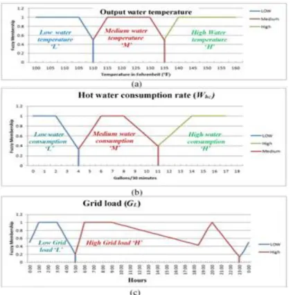
3. The illustrations of the fuzzy membership functions: (a) 𝑓(𝑧,1)(∙) for 𝑇ℎ, (b) 𝑓(𝑧,2) (∙) for 𝑊ℎ𝑐, (c) 𝑓(𝑧,3)(∙) for GL. ...38
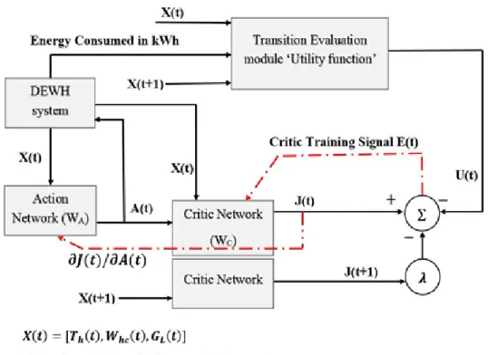
4. (a) Critic adaptation in ADHDP/HDP. This is the same critic network in two consecutive moments in time. The critic’s output J(t+1) is necessary in order to give us the training signal γJ(t + 1)+U(t), which is the target value for J(t). (b) Action adaptation. X is a vector of observables, and A is a control vector. We use the constant ∂J/∂J= 1 as the error signal in order to train the action network to minimize J. This figure is adapted from [20]. ...39
5. Implemented ADHDP controller’s structure. ...39
6. ADHDP Critic Network Adaptation. ……… ...40
7. Q-learning’s schematic diagram. ...40
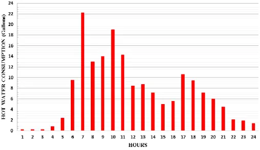
8. Sample user profile generated from the event driven simulator. ...41
9. Extreme user profile used in Experiments 6 and 7. ...41
10. Aggregated energy consumed by all approaches during exp.1...42
11. Aggregated energy consumed by all approaches during exp.2...42
12. Aggregated energy consumed by all approaches during exp.3...43
13. Aggregated energy consumed by all approaches during exp.6...43
PAPER II 1. Overview of ensemble statistical and two-phase feature-based subspace clustering model…… ….………...59
2. Plot of canonical variable for clustering solution 1. ……… ...59 3. Biplot of the canonical variables scores vs. clusters for clustering solution 2.……… .60 4. Biplot of the canonical variables scores vs. clusters for clustering solution 3. ...60 PAPER III
1. Overview of robust unified learning model for clustering unlabeled data, extracting statistically significant features and informing a prediction model. ...83 2. Visualization of multidimensional clusters obtained from analysis of neuroimaging
data of otherwise healthy adults using principal component analysis (PCA)………...83
PAPER IV
1. Regression plots of the MLPANN model for training, validation, testing, and all datasets………. ...112 2. Performance of the training, testing, and validation model (a), and residual of the
MLPANN models (b). ...113 3. Results of intelligentMLPANN model for predicting TSCF based on training,
validation, testing, and all dataset ...114 4. Relationship between Log Kow and MW with TSCF using adaptive network fuzzy
inference system…………. ...115 5. Relationship between Log Kow and HBD with TSCF using adaptive network fuzzy
inference system… ...116 6. Relationship between Log Kow and RB with TSCF using adaptive network fuzzy
inference system… ...117 7. Resulting clusters from using k-means algorithm to generate 3 clusters (k=3), note
that clusters 3 is very distant from the other data samples which clustered as one cluster when k=2… ...118 8. Three dimensional representation of the data used in the clustering ...119
LIST OF TABLES
Table Page PAPER I
1.System states encoding (L: low=0, M: Medium=1, H: High=2) ...36 2.The optimum policies selected by q-learning (1= On, 0= Off) ...36 3.Simulation results from different experiments using the same user profiles in
training and simulation ...36 4. Simulation results from different experiments using user profile in fig. 8 for
training and the profile in figure 9 in evaluation ...37 PAPER II
1.Summary of ASD phenotype features; pairwise correlation; EM uni-dimensional clustering & univariate analysis ...58 2.Top 3 clustering configurations by validation index and multivariate discriminant analysis result ...58 3.ASD severity analysis of clustering solution 1 ...59 PAPER III
1. Discriminant features outcomes of cluster analysis using sMRI features ...80 2. Classification performance of SVM prediction model. ...80 3. Discriminant features outcomes of cluster analysis using qtdMRI features ...81 4. Discriminant features outcomes of cluster analysis using combined qtdMRI
features……… ...82 5. Demographics per cluster……… ...82 PAPER IV
1. Characteristics of measured parameters used in the NN modeling process ...110 2. Results of the MLPANN models with different architectures ...111
3. Results of compounds sensitivity analysis ...111 4. Evaluation for clusters resulted from using different clustering algorithms ...111 5. Evaluation for clusters resulted from choosing different TSCF threshold using
1. INTRODUCTION
1.1.BACKGROUND
The continuous growth in population all around the globe adds new challenges to multiple aspects of life, including the increase in demand on power and better healthcare. These challenges and others require nontraditional solutions that are robust and reliable. Machine-learning algorithms provide the required resources for such solutions due to the revolutionized and adaptive nature of most of these algorithms. Machine learning has become the leading approach in scientific discoveries and innovations that has moved civilization forward in all fields. Machine-learning applications are the reason behind many inventions that are available to us in daily life such as human-machine vocal communication (i.e., speech understanding), machine vision, automatic navigation, route planning, customer segmentation, credit card fraud detection, data mining, internet routing, face recognition, digitization, and medical diagnoses.
Energy management is one of the most challenging problems for power companies. Demand side management is essential in smoothing the grid load profile, which leads to stable and lower cost. Load management techniques have focused on controlling domestic electric water heaters since they have the ability of storing energy. Surveys and official reports show that the load resulting from electric water heaters represents 18% and 23% of the total grid load in the domestic sector in the United States and India, respectively. The peaks in the total grid load profile match those of the electric water heaters’ load profile. The peak load management is vital in controlling the total grid demand. Therefore, several approaches have been applied to control domestic electric water heaters. Some studies
shifted the operation of the electric water heaters unconditionally outside load peak periods. Others prioritized their operation after the peak load periods over one or two hours.
The described problem is a multi-objective problem. Solving such problems requires adaptive and robust algorithms. Reinforcement learning (RL) approaches are efficient in solving such problems. Approximate dynamic programming and simulation-based approaches have shown impressive performance in solving high-dimensional problems within a feasible amount of time.
In addition to the energy management in metropolitan cities, healthcare has become a challenging and attractive field for researchers. In recent years, many studies invested machine learning in healthcare industry and biomedical applications such as early disease detection, monitoring devices, and tracking devices. Healthcare and pharmaceutical companies invests billions of dollars annually to improve the quality of their products. The majority of these investments go for funding advance research centers and developing innovative technologies in the field. Due to the advanced tracking and imaging devices, large datasets are generated to record various types of information ranging from clinical test results to routine questionnaires. The biomedical datasets are heterogeneous in general and need advanced preprocessing. The heterogeneity of clinical datasets exists in patient characteristics, illness severity, and treatment responses. Therefore, clustering becomes the most convenient method for understanding and analyzing the heterogeneous clinical data. Clustering is effective in exploring such complex data and identifying important subsets. In general, machine learning aim to discover unknown patterns or relationships that infer new knowledge that can be further used for prevention, prognosis, and treatment.
1.2. REINFORCEMENT LEARNING
Reinforcement learning is a simulation-based dynamic programming approach that can solve complex sequential decision-making problems such as Markov and semi-Markov decision process. Markov decision process (MDP) models are widely used for modeling sequential decision-making problems that appeared in various fields of science and research. However, many real-world problems modeled by MDPs have large state and/or action spaces, leading to the well-known curse of dimensionality and the curse of modeling, which make solving these models infeasible using dynamic programming. Dynamic programming finds the optimal solution for Markov decision problems, but it needs the transition rewards, transition probabilities, and transition times. These values are almost impossible to determine in most cases. Therefore, machine learning methods such as reinforcement learning are used to determine a suboptimal solution for MDPs. The trade-off between finding a suboptimal solution and the optimal solution is necessary when looking into the massive resources and amount of time required to solve high-dimensional problems using standard methods.
1.3. CLUSTERING
Clustering, also known as unsupervised learning, is a field of machine learning that explores and reveals hidden structures in datasets. Recently, clustering has become more important than ever due to the unprecedented increase in data from various disciplines. Therefore, domain experts are no longer able to analyze such massive datasets and the need for automated approaches and machine-learning techniques becomes imminent. Clustering aims to group data samples into distinctive, compact, and homogeneous groups called
clusters. There is no formal definition for a cluster, but it can be described as a group of data samples that share common features with each other more than they do with samples in other clusters. The process of exploring these datasets often leads to groundbreaking discoveries, such as unexpected causes for a specific phenomenon, or a group of samples that requires attention.
Many clustering algorithms are available for data analysts; therefore, selecting the proper one among them is challenging. Choosing a clustering algorithm depends on the nature of the dataset. However, several metrics can be used to evaluate clustering algorithms. There are three types of cluster evaluations: internal criteria, external criteria, and relative criteria. These evaluation techniques are important in determining the quality of the resulting clusters and evaluating the performance of the applied clustering method.
1.4. RESEARCH OBJECTIVES AND CONTRIBUTIONS
In this work, several improvised machine-learning techniques and algorithms were implemented in the areas of smart grid and biomedical data analysis. The first area includes novel approaches in demand side management. In demand side management, a novel modeling approach is implemented to mitigate the peaks in grid load profile by using adaptive control algorithms, such as Q-learning and action dependent heuristic dynamic programming, to control the domestic electric water heaters. The implemented approach includes several novel techniques that were used for the first time in this optimization problem:
An embedded event-driven simulator was designed to simulate each household hot-water consumption rate.
The control operation of the domestic electric water heater was modeled as a Markov decision process and solved using reinforcement learning.
Novel approaches were implemented to estimate water temperature and to identify system states.
The problem was modeled as a multi-objective optimization problem, with the goals of reducing energy cost and smoothing load grid profile while maintaining desirable temperature for the supplied water.
The implemented approach has the potential to be utilized in the internet of things.
According to the simulation results, the approximate dynamic programming approaches (Q-learning and action dependent heuristic dynamic programming) outperformed all other scenarios in terms of cost reduction, while maintaining desirable water temperature.
In the area of biomedical data analysis, this dissertation presents three papers. Each paper applied enhanced and improvised clustering techniques on specific biomedical datasets. The first paper in this area (Paper II), implements an ensemble statistical and subspace-clustering model to analyze autism spectrum disorder (ASD) phenotypes. This dataset is challenging due to the complex heterogeneity it conveys from the variability in behavioral phenotypes as well as clinical, physiologic, and pathologic parameters. In this paper, a new k-dimensional subspace-clustering algorithm is presented and used to analyze
and cluster the autism dataset. This algorithm is part of the general model that was implemented in this project. The implemented approach is general and can be applied to other biomedical datasets. It incorporates several statistical methods at different levels of the model. The implemented approach successfully sorts out the heterogeneity in the ASD dataset and produces clinically meaningful clusters. This approach is useful in understanding and studying etiology, diagnosis, treatment, and prognosis of ASD.
The second paper (Paper III) in this area applied a robust unified learning framework to cluster subgroups using neuroimaging data for brain volume and white matter. This unified model was used to identify neurological phenotypes that can sort the heterogeneity in cognitive aging and help identify potential risk factors for suboptimal brain aging. The use of machine-learning approaches identified two unique subgroups in healthy older adults with different patterns of white matter integrity and brain volumetric measures. The implemented model identified significant measurements that could potentially serve as biomarkers for delineating clinically meaningful aging subgroups.
The last paper (Paper IV) used machine-learning techniques to study the effect of contaminants and chemical compounds on plant uptake and the causes of pollutants transportation from the environment to vegetation and food. Several approaches were implemented in this paper: neural networks (NN), fuzzy logic, clustering, and statistical methods. The NN model was built to predict transpiration stream concentration factor. Fuzzy logic and clustering were used for predicting TSCF using physicochemical properties of compounds, and examining the interactions between compound properties. Several clustering algorithms have been applied, and they all discovered two major distinct clusters. The clusters resulting from k-means algorithm were the most significant and only
these are presented. Physiochemical property cutoffs, i.e. restrictions, for compounds passing plant roots membrane were shown to be lower than the cutoffs for transmembrane transport in mammalian intestinal systems. Therefore, the human health impacts through consumption of contaminated crops is elucidated and indicated that plant roots are a restrictive barrier to organic pollutants entering our foods. Improved understanding and prediction of plant uptake has significant implications for human health as we continue to shorten our water cycles.
PAPER
I. DEMAND-SIDE MANAGEMENT OF DOMESTIC ELECTRIC WATER HEATERS USING APPROXIMATE DYNAMIC PROGRAMMING
Khalid Al-jabery, Zhezhao Xu, Wenjian Yu, Donald C. Wunsch, II, Jinjun Xiong, and Yiyu Shi
ABSTRACT
In this paper, two techniques based on Q-learning and action dependent heuristic dynamic programming (ADHDP) are demonstrated for the demand-side management of domestic electric water heaters (DEWHs). The problem is modeled as a dynamic programming problem, with the state space defined by the temperature of output water, the instantaneous hot water consumption rate, and the estimated grid load. According to simulation, Q-learning and ADHDP reduce the cost of energy consumed by DEWHs by approximately 26% and 21%, respectively. The simulation results also indicate that these techniques will minimize the energy consumed during load peak periods. As a result, the customers saved about $466 and $367 annually by using Q-learning and ADHDP techniques to control their DEWHs (100 gallons tank size) operation, which is better than the cost reduction that resulted from using the state-of-the-art ($246) control technique under the same simulation parameters. To the best of the authors’ knowledge, this is the first work that uses the approximate dynamic programming techniques to solve the DEWH’s load management problem.
INDEX TERMS
Approximate dynamic programming (ADP), load management, machine learning, Markov processes, power demand, smart grids, unsupervised learning.
1. INTRODUCTION
The importance of domestic electric water heaters (DEWHs) can be seen from its effect on the overall grid load and energy consumption. For example, in the U.S. the average energy consumed by DEWHs is 18% as shown in Fig. 1. This share did not change during the last decade according to the U.S. Energy Information Administration [1]. The average annual cost of energy consumed by each DEWH is about $500 according to the office of energy and renewable energy [2]. Previous and current researches show that the total energy consumed in a city is highly dependent on the amount of power that the DEWHs consume [3]–[7]. For example, in the city of Quebec, Canada, the peaks in the grid load depends on the water heaters load, as illustrated in Fig. 2. The data plotted in Fig. 2, are from the field studies performed in two different cities [3], [4]. There is a clear relationship between the peaks in the grid load demand and those in the energy consumed for heating water in London and Quebec City. As a result, governmental agencies, policy makers, and of course energy companies, focus on domestic energy consumption with high priority for the water heaters. On April 30, 2015, president Obama signed into law S535, The Energy Efficiency Improvement Act, which established a new product category for large-capacity (75 + gallons) electric resistance “grid-enabled” water heaters for residential demand-response applications. Before that in the 15th of April, the Department of Energy
provided new rule that requires all large capacity (55+ gallons) DEWH would have to be integrated electric heat pump water heaters. The current trend of research according to the peak load management agency is to design efficient grid enabled water heater, which is exactly what we have produced in this paper [8]. The attention to water heaters and load management is not only in the U.S. According to the reports of the Ministry of Power in India, DEWHs consumes nearly 23% of the electricity in the domestic sector [9].
The DEWHs are often selected for demand side management projects because both their load profiles and their average daily load profiles almost follow the same pattern as shown in Fig. 2. Furthermore, DEWH loads are easier to control than other domestic appliances, because of their energy storage ability. Although many researches have been conducted on DEWHs, most of them failed to be widely applied to the DEWH industry for various reasons. There are different demand side management strategies for controlling DEWH loads. In 1998, Nehrir et al. [6] introduced a fuzzy logic controller that can shift the DEWH load outside the peak demand period. Some of the suggested approaches significantly affected the temperature of the DEWH’s output water, resulting in customer dissatisfaction, plus the complex modeling process it needs [7]. In 2007, Atwa et al. [10] used Elman neural network to control the power consumed by water heaters. Some researchers, used detailed analytical methods for modeling the DEWH and provided control strategies based on dividing the load into groups and control them through the thermostats [10]–[17]. In 2011, Moreau [3] described control strategies aimed at distributing and shifting DEWH’s operation to within one or two hours outside the peak periods. The new coming technology in water heaters industry is the use of electric heat pump and gas condensing technology for water heaters with tanks that are larger than 55
gallons [18]. However, there are three concerns raised on this new technology, first it needs new installations, second it tends to be used in water heaters with large tanks only. The third concern and the most important one is low temperature operation when the heat pump water heater operates in electric resistance mode, it does not save energy or money compared to a conventional unit [19]. Even if the new heat pump water heaters dominated the market, the approaches demonstrated in this paper still can be used to improve the performance because they are designed to adapt with the user activities, grid load and the temperature of the output water as discussed next.
In this paper, we used action dependent heuristic dynamic programing (ADHDP) [20] and Q-learning approaches to solve the DEWH management problem, which is a multi-objectives optimization problem. The objectives are: minimizing the total cost of the energy consumed, reducing the load demand during peak periods, and achieving customer’s satisfaction. The Q-learning algorithm and the ADHDP approach are both approximate dynamic programming (ADP) techniques [20], [21]. It should be pointed out that this paper is the first study using ADP techniques in the DEWH’s load management.
The novelty of this paper lies in the way that the system is modeled. Three factors were used to define and control a DEWH: 1) the temperature of the water delivered to the customers; 2) instantaneous hot water consumption; and 3) estimated grid load demand (i.e., instantaneous energy price). In the Q-learning based approach, the three factors are considered linguistic variables. They are categorized as either “high,” “medium,” or “low.” The problem was modeled as a semi-Markov decision process (SMDP) with two possible actions in each state: 1) “ON” and 2) “OFF.” Specific fuzzy rules are used to determine the system’s current state. Each DEWH is considered to be an artificial agent that was trained
to adapt to the diversity within a user’s consumption profile and grid load demand. The agent learns how to adapt, in the Q-learning approach, after finding the final Q-factors that specified the operating’s policy during real time operation. In the ADHDP approach, the adaptation process consists of two phases: 1) critic training and 2) action training. The system learns to estimate the correct cost value during training the critic network, and then uses that cost in training the action network. The system tries to minimize the cost by adapting the weights of the action network [20].
These techniques can be applied to any DEWH, regardless of its capacity, heating elements, or operating environment. Furthermore, according to the simulation results, the approaches are able to reduce the energy consumed by DEWH more than the existing state-of-the-art methods [3]. The experiments show that the Q-learning and ADHDP controllers have reduced the cost of the energy consumed by the DEWHs by approximately 26% and 21%, respectively when using large (100 gallon tank) DEWH. As a result, both techniques will save about $466 and $367 per year, respectively, for the customers who use them to control their DEWH’s operation. In comparison, only $246 would be saved annually by using the state-of-the-art control strategy [3], as illustrated in Table 3.
2. SYSTEM MODELING AND THE APPROXIMATE DYNAMIC
PROGRAMMING
ADP techniques have been used effectively in solving optimization problems that consist of sequences of control actions whose efficiency remains unknown until the end of sequence. For the demand side management problem of DEWH, two ADP techniques: 1) ADHDP and 2) Q-learning (which is a special case of ADHDP) [20], were considered. The
system modeling, and the training and controlling processes of both techniques are explained in the following sections.
2.1. SYSTEM MODEL
The DEWH model is defined by three variables: the output water temperature (Th),
Hot water consumption rate (Whc), and the grid load (GL). Whc is generated randomly (See
Section 3.3), Th is calculated using (2) and (3) based on the selected action, GLdependson
the city grid load profile. Therefore, the three variables are not correlated. However, the values of these variables were used differently for the two approaches presented in this paper.
In the Q-learning based approach, the variables were converted in to linguistic values using fuzzy membership functions, as illustrated in Fig. 3. The variables (Th and
Whc) have three possible values (low ‘L’, medium ‘M’ or high ‘H’) while GL has only two
possible values low or high. (This assumption was based on the time-of-use ToU pricing profile that is used in this paper where there is no medium grid load or in other word medium power cost also it is meaningless practically to describe grid load as medium).
Therefore, a discrete state system can be defined with 332=18 different states. The demand side management problem is to decide whether to turn the DEWH “On” or “Off” at each event time, which refers to the time when user consumes any quantity of water from the DEWH’s tank. In practice, the numeric value of each variable should be fuzzified and mapped to its corresponding linguistic value. The fuzzy membership functions 𝑓𝑧,𝑖(∙), (𝑖 = 1,2, 3) are defined for the three variables, and illustrated in Fig. 3. For variables Th and Whc, values of L, M and H correspond to 0, 1 and 2 respectively. For
variable GL, the values of L and H correspond to 0 and 1, respectively. The water
temperature thresholds were specified based on the fact that legionella bacteria begin to die at temperatures above 120° F [22].
Suppose 𝑣1, 𝑣2 and 𝑣3are the numeric values of the three variables respectively, and 𝑆(𝑣1, 𝑣2, 𝑣3) is the corresponding state’s index number. Then,
𝑆(𝑣1, 𝑣2, 𝑣3 ) = ∑3𝑖=1[3𝑖−1𝑓𝑧,𝑖(𝑣𝑖)]+ 1 (1)
The system states are encoded as listed in Table 1.
Equation (1) is used to determine the system’s current state during the training phase. It is used during the simulation as well. The linguistic values are vital for calculating the immediate reward during training (see Section 3). Actions are selected randomly with equal probability during the training phase in order to provide stochastic value iterations and update the Q-factors accordingly. As discussed in Section 3.2.
Variable Th's numeric value at time (t+1), denoted by 𝑣1(𝑡 + 1) can be estimated
based on the action decision made at time (t). From the law of energy conservation [23], [24], we derive: 𝑣1(𝑡 + 1)|𝑎(𝑡)=1 = 9𝑃𝜏 5𝐾𝑗𝑉∙ 𝑚1𝐶ℎ𝑤𝑇ℎ(𝑡)+[𝐶𝑐𝑤𝑇𝑐−𝐶ℎ𝑤𝑇ℎ(𝑡)]∙𝑚2(𝑡) 𝑚1𝐶ℎ𝑤+(𝐶𝑐𝑤−𝐶ℎ𝑤)∙𝑚2(𝑡) + 32 , (2) 𝑣1(𝑡 + 1)|𝑎(𝑡)=2 = 9 5∙ 𝑚1𝐶ℎ𝑤𝑇ℎ(𝑡)+[𝐶𝑐𝑤𝑇𝑐−𝐶ℎ𝑤𝑇ℎ(𝑡)]∙𝑚2(𝑡) 𝑚1𝐶ℎ𝑤+(𝐶𝑐𝑤−𝐶ℎ𝑤)∙𝑚2(𝑡) + 32 , (3) where v1(t)is the current temperature of the water, a(t) is the current action, 1 means “On”
and 2 means “Off”. m1 is the total mass of water in the DEWH tank, m2(t) is the mass of
water consumed at the time (t), and m2(t)= v2(t)3.785[25]. Chw and Ccw represent the heat
supplied to the DEWH, typically 10~13 ͦ C [26]. P is the power rating of the heating element (4500, 2800 or 36000 Watts per hour in this study). Kj =2.42 W*h/gal*℉, which
is the recovery rate calculation constant [27], [28], and V is the total volume of the DEWH tank. τ is the sampling period (30 minutes in this study). v1(t) and v1(t+1) are in unit of ℉.
Heat dissipation and heat exchange between the DEWH metal surface and air is negligible (less than 0.25 ℃/hour) [19]. These two equations are to estimate the water temperature using energy saving formula. According to the behavior and ranges of the calculated temperature at each time step in compare with field studies [3]-[5], the model was acceptable. However, accurate performance to these models have not presented in this work. Due to the involvement of several random functions in profiles generation and the absence of real data.
An event driven simulator was designed to generate users’ profiles. The simulator mimics the data that were collected in [3] and [4]. The distribution fitting toolbox in MATLAB was used in this study to determine the random variable distribution. The designed event driven simulator generates the time of the events (which specifies the current grid load GL) and the quantity of hot water used in each event Whc. The linguistic
value of the grid load factor (GL) is determined based on the event time since previous
studies have shown that there are specific periods during the day when the load demand becomes high [3]-[7], [13]. However, a time-of-use (ToU) pricing profile is used to calculate the real cost of the consumed power [29] as illustrated in Section 3.3. The instantaneous output water temperature, Th, is calculated using (2) and (3) when the
selected action at time (t) is “Off” and “On” respectively. One of the advantages of the approach is that it avoids the complicated thermodynamic and heat transfer operations,
which occur inside the DEWH’s tank, by using (2) and (3) to estimate the value of Th at
time (t+1). Furthermore, the presented work does not require any complex calculations such as that described in previous studies [7] to solve the optimization problem.
In the ADHDP approach, the system is modeled as a continuous state space system. The system’s state is also defined by the same variables (Th, Whc, and GL) used in the
Q-learning approach, but there is no fuzzification/ defuzzification process. The state variables are the inputs of the Critic and the Action neural networks in the ADHDP controller. Their normalized numeric values are used to train the neural networks. This will be explained in more detail in Section 3.1.
2.2. APPROXIMATE DYNAMIC PROGRAMMING
Approximate or Adaptive Dynamic programming (ADP), also known as the reinforcement learning, simulation-based dynamic programming, stochastic programming, and neuro-dynamic programming, refers to a group of algorithms designed to solve the problem of Markov and semi-Markov decision processes given by (4) [30].
𝐽∗(𝑖) = max
𝑎∈𝐴(𝑖)[∑ 𝑝(𝑖, 𝑎, 𝑗)[𝑟(𝑖, 𝑎, 𝑗) + 𝜆𝐽 ∗(𝑗) |𝑆|
𝑗=1 ], (4)
where J*(i) is the i-th element of the vector value function associated with the optimal policy. A(i) is the set of all actions allowed in state i, p(i, a, j) represents the transition probability of going from state i to state j under the influence of action a. r(i, a, j) is an immediate reward earned when action a is selected in state i and the system transfers to state j as a result. S represents the set of states in the Markov chain, and λ is the discounting factor.
2.3. Q-LEARNING ALGORITHM
Watkins published the Q-learning algorithm in 1989. He defined this method as “a form of model free reinforcement learning and it can be viewed as a method of asynchronous dynamic programming” [31]. The Q-learning algorithm associates a scalar value, the Q-factor, with each state action pair. It solves (4) by updating the Q-factors associated with an optimal policy instead of approximating the cost function of a particular policy. Furthermore, it uses policy iteration (PI), as described in (5), to avoid the evaluation of multiple policies. The PI serves as the Q-factor version of the Bellman equation [21], [30].
𝑸(𝒊, 𝒂) = ∑ 𝒑(𝒊, 𝒂, 𝒋)[𝒓(𝒊, 𝒂, 𝒋) + 𝝀 𝐦𝐚𝐱
𝒃∈𝑨(𝒋)𝑸(𝒋, 𝒃)] |𝑺|
𝒋=𝟏 , (5)
where Q(i, a) and Q(j, b) are the Q-factors associated with state-action pairs (i, a) and (j,
b), respectively.
Equation (5) still requires the transition probabilities. Therefore, the Robbins-Monro algorithm [32] was used to estimate the optimal Q-factors. The optimal Q-factors’ estimation was achieved by expressing every Q-factor as an average of a random variable. Equation (6) represents the Q-factor version of the value iteration, which is the Q-learning algorithm for a discounted Markov Decision Process (MDP). The derivation of (6) from (5) can be found in [30].
𝑸𝒏+𝟏(𝒊, 𝒂) = (𝟏 − 𝜶𝒏+𝟏) 𝑸𝒏(𝒊, 𝒂) + 𝜶𝒏+𝟏[𝒓(𝒊, 𝒂, 𝒋) + 𝝀 𝐦𝐚𝐱
𝒃∈𝑨(𝒋)𝑸(𝒋, 𝒃)], (6)
where αn+1 represents the adaptive learning rate and attenuating with time. Qn+1 is the
Algorithm 1: Q-learning
1 Set up the training parameter: imax, and initialize Q-factors=0 and t=0. 2 Randomly select initial state and action (S0,a0).
3 Repeat until (number of iterations > imax).
Apply action a(t) on DEWH model and read the current and the estimated values
of vi(t) and vi(t+1), respectively.
Determine S(t+1) using (1).
Calculate immediate Reward r(St,at,St+1)
Update Total Reward Rt=Rt+ r(St,at,St+1).
Update: t=t+1; S(t-1)=S(t);S(t)=S(t+1).
aUpdate learning rate: 𝜶 = 𝜶𝒕+𝟏.
Update Q-factors using (6).
4 Construct the final policy from (S, a) pairs with higher Q-factors using the following formula on each state (i):
𝑷(𝒊) = 𝒂𝒓𝒈𝒃∈𝑨(𝒊)𝒎𝒂𝒙 𝑸(𝒊, 𝒃); 𝑷(𝒊) is the policy at state (i) (i.e. action that lead to maximum reward on the long run).
5 Record 𝑷̂(optimum policy for all states) and stop.
a There are multiple ways to update the learning rate (α) [21]. In this work, we update 𝛼
using: 𝛼𝑡+1 =𝑐𝑐1
2+𝑡, where the positive constants 𝑐1 and 𝑐2fulfills 𝑐1 < 𝑐2. (e.g. we set 𝑐1 =
200 𝑎𝑛𝑑 𝑐2 = 220. More discussion on learning rate selection can be found in [21]). In this study, the Q-learning version of the value iteration was used to solve the pre-described SMDP problem, which can be viewed as a discounted reward for the reinforcement learning based on the stochastic value iteration. However, the Q-learning version used in this paper uses a specific cost function to generate the immediate cost/reward for each system state transition, as illustrated in Section 3.1. This cost function eliminates the need for the transition reward matrix TRM, which is usually used in Q-learning algorithms. The same cost function was used to evaluate the system’s transition in the ADHDP approach as well (See Section 2.4).
2.4. ACTION DEPENDENT HDP
The family of adaptive critic design (ACD) controllers has been presented by Werbos [33]. HDP, and its action dependent ADHDP forms, have a critic network that estimates the cost-to-go function J* in (4) which calculates the Bellman equation of dynamic programming [20]. The standard structure of HDP and ADHDP is illustrated in Fig. 4. ADHDP is a generalization of Q-learning for the continuous domain system. In ADHDP, the critic is trained to provide an accurate estimation for the cost-to-go function J and to minimize the following error E(t):
𝐸(𝑡) = 𝐽[𝑋(𝑡)] − 𝛾𝐽[𝑋(𝑡 + 1)] − 𝑈(𝑡), (7) where X(t) is the vector of observations/variables that define the system’s current state.
The ADHDP controller adaptation process consists of two phases: Critic and Action networks training. These two processes are implemented continuously in sequence but not in parallel.
The critic network is designed to minimize a back propagated error signal (7), and the gradient of J with respect to the weights of the critic Wc is given by:
Δ𝑊𝑐 = −𝜂𝑐[𝐸(𝑡)] × 𝜕𝐽
𝜕𝑊𝑐, (8) where 𝜂𝑐 is a positive learning rate (0 < 𝜂𝑐 ≤ 1). The action network is connected as shown in Fig. 4(b) in order to minimize J in the next time step and optimize the total cost over the entire domain. In the action network’s adaptation phase, the gradient of J with respect to A (i.e. 𝜕𝐽/𝜕𝐴) is back propagated as illustrated in Fig. 4(b) and in (9):
Δ𝑊𝐴 = −𝜂𝑎 ×𝜕𝑊𝜕𝐽
𝐴 , (9) where 𝜕𝐽/𝜕𝑊𝐴 = (𝜕𝐴𝜕𝐽) × (𝜕𝑊𝜕𝐴
the weights of the action network WA. 𝜂𝑎 is the action network learning rate ( 𝜂𝑎 doesn’t
have to be equal to 𝜂𝑐 in (8.)
In HDP the immediate cost or the utility function U(t) is approximated as well using neural networks, while in ADHDP, U(t) is calculated using a model and the action network is connected directly to the critic [20]. The approaches described in this paper were designed to overcome the limitations presented by previous solutions. These improvements focused on the following:
Reducing the need for permanent communications and synchronizations between DEWHs and the smart grid infrastructure [7], [12].
Either shifting or eliminating the peaks with in the grid load [3].
Reducing power consumption during peak periods and as a result minimizing the cost of the power consumed without sacrificing customer satisfaction.
3. TRAINING AND IMPLEMENTATION
This section contains the discussion on the processes required to transform a normal DEWH into a smart appliance. The discussion clarifies and compares the technical implementation of the presented approaches: the ADHDP and the Q-learning.
3.1. ADHDP IMPLEMENTATION
The ADHDP controller is illustrated in Fig. 5. It consists of the following components:
The DEWH system module: which was described in (2) and (3) is the same module used during Q-learning and the final simulation (to be discussed further in Section 3.2 and Section 4).
The critic network used in this work consists of: one input layer with four neurons (for each state variable and the action network output), one hidden layer with 30 neurons each of which has a hyperbolic tangent sigmoid activation function, and one neuron in the output layer with a linear activation function. The output of the critic is J(t), if the inputs were X(t) and A(t) or J(t+1) if the inputs were X(t+1) and A(t+1).
The action network is almost identical to the critic network, but it only has three neurons in the input layer, and the sigmoid activation function is used in the hidden and also the output layer. The action network generates the control action (On or Off) during normal operation and simulation.
The transition evaluation module (or utility function) was designed to replace the TRM as illustrated in Section 2.3. This utility function (in some literature called a cost function) calculates the immediate transition reward/cost for each system’s state transition. The same function was used in Q-learning as well. The utility function provides a more efficient evaluation than the TRM. The utility function calculates the immediate transition cost based on the energy consumed during the transition and all the other control variables (Th(t), Whc(t), GL(t)), as illustrated in Algorithm 2. The pseudo code of the cost function
illustrated in Algorithm 2 is of major importance because it highly reduced the complexity of the training process for both ADHDP and Q-learning compared to previous work [34]. The utility function rewarded the agent for each gallon of output water supplied with Th >
but that penalty depends also on whether it was consumed during peak or normal load. If
GL is low, the penalty will be mitigated through dividing the kWh by (𝑎) and vice versa,
as illustrated in Algorithm 2. The guidance factors (𝑎 𝑎𝑛𝑑 𝑏) provide control over the multi-objective optimization process. (i.e. they encourage the agent to turn the heating element on during low load periods and to reduce the effect of the different scale between energy and output water units). Experimental results showed that: choosing 𝑎 𝑎𝑛𝑑 𝑏 such that (𝑎 ≥ 2𝑏, ∀𝑏 ≥ 1), provides better performance for the ADHDP controller. However, these factors have no effect at all on the Q-learning performance, as illustrated later in Table 3.
Algorithm 2: Utility function
Calculate_cost(power in kwh, state: X(t)= [Th, Whc, GL], t) 1 if GL is high
J=energy in kwh*a; % penalty P1 {peak load}
if Th< threshold
J=J+Whc; % increase cost {penalty} else: J=J-b*Whc; % decrease cost {reward} 2 else
if time (t) is between 3 and 5:30 am
J= energy in kwh/a; % P2<P1 low load Else
J= energy in kwh/b; % P1>P3>P2 if Th< threshold
J=J+Whc*a; % increase cost {penalty} else: J=J-Whc; % decrease cost {reward} 3 If Q_learning % see Section 3.1
J=-J; 4 Return J;
The adaptation of the presented ADHDP controller was implemented in two phases:
Offline training:In the offline training, the critic network was trained first using the data generated from the Q-learning algorithm. The critic training stops when the back
propagated error signal from (7) becomes less than a pre-specified small value, or when the training lasts for the maximum number of iterations. The critic training of the presented ADHDP is illustrated in Fig. 6. Furthermore, the action network is also trained during the offline phase using the same data used in critic adaptation. The size of the data sets depends on for how many simulation days Q-learning was trained, and each day contained about 150 samples. It was noted during experiences that repeating the offline training after the online training enhances the ADHDP controller’s performance. The selection of the guidance factors has major effect on the ADHDP performance too as illustrated in Sections 4 and 5.
Online training:The online training is executed during the simulation phase. The action network keeps adapting during the simulation to minimize the system’s cost to go (i.e.,
J). Simulation here is the same as real time operation, because of the use of the event driven simulator that explained in Section 4. The adaptation of the action network is illustrated in Section 2.4.
The presented ADHDP controller showed better performance in cost reduction as the number of iterations increased. The critic adaptation is illustrated in Fig. 6 and was recorded during training for 100 simulation days with a total data set size of about 15000 samples.
3.2. Q-LEARNING IMPLEMENTATION
The second optimization approach implemented in this work is the Q-learning algorithm. The actions are selected randomly with equal probability at each time step to achieve better exploration of the solution space during the training phase. The algorithm
then receives the control variables’ estimated values at (t+1) from the DEWH model and evaluates the performed action based on the utility function illustrated in Algorithm 2, which is the same utility function used in ADHDP. In step 3 from Algorithm 2, the calculated cost is negated. This is because Q-learning selects the optimum policy based on the Q-factor with the maximum value, unlike ADHDP which seeks to minimize the cost. The Q-factor associated with (𝑺𝒕, 𝒂𝒕) was last updated using (6). This algorithm repeats the same procedures and continues until the maximum number of iterations are performed. The Q-factors have been stored in an (18x2) scalar matrix. The optimum policy is then derived, as illustrated in Algorithm 1 and Fig. 7.
Each iteration here represents a one-day simulation that contains about 150 time steps based on the event driven simulator used. The best value for the discount factor 𝛌 was derived heuristically as 0.9. Note that the same notation used in Fig. 5, to indicate the fact the same discount factor was used in ADHDP as well. The training phase for both of the presented approaches (ADHDP and Q-learning) was conducted using a DEWH’s module with the following parameters:
1) The heating element power= 36, 4.5, 4.5 or 2.8 kWh.
2) Tank size=120,100, 70 or 40 gallons respectively. 3) Discount factor 𝜆=0.9.
The state’s variables linguistic values were derived as illustrated in Fig. 3, for Q-learning. The same specifications were used with in the simulation for all the other simulated approaches as well.
3.3. DATA PROCESSING
This section includes discussion on the process of generating the control variables’ numerical values (Th, Whc, and GL) and illustrates the event driven simulator.
The event driven simulator presented in this work provided comparable results with those obtained from previous field studies [3], [7]. The simulator is designed to mimic human activities in consuming hot water. This simulation was required to provide a reliable assessment for the presented DEWH’s control approaches. The simulator generates (per simulation day) unique and random profiles for each DEWH used in the simulation as shown in Fig. 8. The simulator assumes 4 occupants in each house, for simplicity we avoided considering the ages, gender, and other social factors for the occupants that may affect their hot water consumption rate. The generated profile shown in Fig. 8, is comparable to the profiles obtained from the field studies in the British Department for Environment, Food and Rural Affairs’ report [4].
The simulation consists of two phases: 1) Profile generation which was used in training and in performance evaluation or comparison and 2) comparator simulator, in which an evaluation process implemented among the presented approaches and the state_of_the_art approaches [3]. The profile’s generator also provides the time of using the hot water and how much hot water was used. In the evaluation phase, different models for the DEWHs were used, uncontrolled “reference”, Scenario0, 1, and 2, Q-learning, and ADHDP. Each group of DEWH have the same number of DEWHs units, the same tank size (120, 100, 70 or 40 gallons) and heating element (36, 4.5 or 2.8 kWh). The simulator assumes that, we are creating six parallel universes or copies from every house dwelling and give each copy different brand (i.e. version) of DEWH. The performance of each group is
evaluated during the simulation based how much energy each group can save with respect to the uncontrolled scenario (All scenarios operated for the same period of time and using the same user profile).
This criteria is used to guarantee a fair comparison among the different approaches. Otherwise, it is difficult to present an accurate comparison among the different control strategies. The user profiles which includes events’ time indices and the consumed hot water quantities were generated using special combination of Poisson random variables. The choice of these variables is based on using the distribution fitting tool box from MATLAB on the previous studies’ data. The profile generator function was adjusted empirically till it provides user profiles similar to the actual user profiles obtained by previous studies [3]-[5]. Artificial profiles needed due to the limitations of real data profiles. The numerical variables used for calculating the variables are explained as follows.
Water temperature: In this work, instead of diving deep inside the thermodynamic operations of the DEWH, we utilized the law of energy preservation to provide a reasonable estimation for the temperature of the output water at the hot water faucet, as in (2) and (3). Since calculating the output water’s exact instantaneous temperature is almost impossible without using an expensive embedded system to calculate the temperature of the DEWH’s output water [23]-[25].
Hot Water consumption rate:Estimating or predicting any human activity is extremely difficult. This study relied on statistics from field surveys, which have been performed in London, UK and Québec, Canada [3], [4]. However, to generate the required data, an embedded event driven simulator was designed as illustrated in the previous section.
Grid Load “Energy Cost”: The estimated instantaneous grid load can be obtained from the local utility companies, and they are time dependent as illustrated in Fig. 3 (c.) As mentioned earlier the grid load characteristics used in this work are based on data obtained from Quebec and London [3], [4]. However, the numeric values of this factor are the time indices of the operation. The load peak periods occurred approximately between 5:30 am and 10:00 am and between 4:30 pm and 10:00 pm. Furthermore, the final comparison was conducted using a time-of-use profile [29].
Energy consumed by the DEWH’s heating element: The amount of the consumed energy is calculated using the module described in (2) and (3). The values of the immediate energy consumption in kWh were used to calculate the value of the utility function at each system transition as illustrated in Figs. 5 and 7.
The control variables’ numerical values are normalized before being used as inputs for the action and the critic networks in the ADHDP controller. The same profiles generated during the Q-learning process were used in the ADHDP approach as well.
4. SIMULATION AND EVALUATION
The simulation process was designed to provide the same operating conditions for all the simulated scenarios as discussed in the previous section. Five different approaches were simulated under the same operating conditions. These operating conditions are as follow:
1) The DEWH specifications as listed in Section 3.2.
3) A soft threshold specified to be 125 ℉. This soft threshold was used to prevent the output water’s temperature to fall below 120 ℉ for all the compared approaches [22] (To maintain customers’ satisfaction.) The DEWH heating element should be turned “On” whenever the water temperature fell below the soft threshold. However, the simulator recorded even the quantities of water outputted to users below thresholds to provide more accurate evaluation to each of the control strategies as illustrated in Tables 3 and 4.
The evaluation comparison is performed among five groups of DEWHs plus the uncontrolled operation as a reference. Each group has the same number of identical DEWHs. The results in this paper were derived from simulating the operation of 100 DEWHs in each group. Any number of DEWHs can be used and from experiences no effect on the comparison. Since the same user profiles is being used for the different groups. In other words: the same group of DEWHs were simulated using 5 different control scenarios and the uncontrolled scenario. The final assessment was presented based on the percentage cost reduction of the consumed energy cost using a ToU pricing profile. The ToU profile gives three different prices for the kWh during the day: 5.62¢, 10.29¢ and 23.26¢ [29]. These prices were applied to the load profile of the city of Quebec that used in this study and the state-of-the-art work that is compared with. As a result, the pricing profile that was used in our comparison simulator is as follow for the energy unit price:
23.26 ¢ for each kWh consumed between 5:30 and 10:30 am (load peak 1.)
10.29 ¢ for each kWh consumed between 4 pm and 9 pm (load peak 2.)
The different scenarios presented in the state-of-the-art work in the field (i.e., Scenarios 0, 1, and 2 in the list) [3], the uncontrolled scenario (i.e., Scenario 4), and our scenarios (scenarios 3 and 6) are all discussed below.
1) Scenario 0: The demand pick-up at the end of the load shifting period is not controlled. 2) Scenario 1: The pick-up is controlled according to a prioritized random function that was spread over a range of one hour after the peak period ended. In this scenario, the agent turns the heating element off during the peak period.
3) Scenario 2: The pick-up is controlled according to a prioritized random function that is spread over a range of two hours after the peak period ended. The success of the simulator can be verified by looking at the energy consumption curves in Figs 10-13.
4) Scenario 3 (Q-learning): The entire operation of every DEWH in the group is controlled according to the policy selected after the presented Q-learning algorithm (also known as the trained group in the comparison charts), which is used to train the agent.
5) Scenario 4 (Ref. or uncontrolled scenario): The DEWHs that are simulated under this scenario are operating under no artificial control. The heating element is turned “On” whenever the water temperature became less than the specified soft threshold and “Off” if it exceeds140 ℉. This scenario (also known as the uncontrolled group in the comparison charts) is used as a reference to calculate the performance of all other scenarios.
6) Scenario 5 (ADHDP): All the DEWHs simulated with in this group are trained, as illustrated in Section 3.1, using the adaptive critic technique ADHDP.
Scenarios 3 and 5 are the techniques implemented in this work. Both scenarios (Q-learning and ADHDP) perform well and even better than the state-of-the-art strategies (Scenarios 0, 1, and 2) in the existing work [3].
In Scenario 0, the agent simply deactivated the heating element during peak periods unless Thfell belowthe soft threshold, which is in this work was 125 ℉. The controller
turned the heating element “On” all the time it was outside the specified peak periods unless their (Th)exceeded the maximum allowed temperature (140 °F). New peaks appeared when
the heating elements for all DEWHs were reactivated simultaneously. In Scenarios 1 and 2, the agent randomly reactivated the water heaters at the end of the load shifting period, giving priority to those that were having the lowest water temperature to be turned “On” first. The time required for the water heaters to reactivate at the end of the shifting load was based on a random function. It was also based on the water’s temperature at the end of the load shifting period.
Scenario 3 and 5 represented the control approaches that were presented in this study. In Scenario 3, the operation of the DEWH’s heating element was entirely controlled by the suboptimal policy that was achieved during the Q-learning’s training phase. The same simulator that generated the control variables during training was used to calculate them during comparison as well.
Furthermore, in all scenarios, the DEWH controller overrode its control scenario on two occasions: when Th either decreased below or exceeded the pre-specified soft-threshold (125 °F) or maximum (140 °F) soft-thresholds, respectively. The soft soft-threshold was used in the comparator simulator in order to guarantee the same degree of customer’s satisfaction for all scenarios (when all scenarios maintained their water’s temperature above the hard threshold of 120 °F. It also provided clear performance measurement for the different scenarios, based on the consumed power cost only. The cost of the consumed power was calculated using a ToU pricing profile [29] as illustrated in Section 3.3.
5. RESULTS
The event driven simulator, the described system’s modelling, the Q-learning process, ADHDP controller back propagation training, and the simulator used for evaluating the performance of all approaches were all designed using MATLAB. Many simulations were conducted in this work using different training parameters. As a result, the best learning schemes for Q-learning in terms of distance between Q-factors and policy stability were obtained using a discount factor of λ=0.9. Table 2 illustrates the optimum policies selected by Q-learning for 30 and 100 iterations for DEWH with tank size 70 gallons.
The learning agent showed the best performance in all experiences. The Q-learning approach implemented here is more advanced and comprehensive than that presented in previous work [34]. The current work uses realistic time events as generated by the event driven simulator. (In the previous work [34], the controller made a decision every 30 minutes). The ADHDP approach is also conducted in all experiments and it outperformed the state_of_the_art approaches [3] when setting the appropriate values for the guidance parameters (𝑎 𝑎𝑛𝑑 𝑏, See Section 3.1). The ADHDP approach is based on the continuous state space version of the problem, not a discrete state space like Q-learning [20]-[21], [30]-[31], [35]. Several experiments were implemented as illustrated in Tables 3 and 4. Table 3 contains results for the experiments that were implemented using the same profiles during training and evaluation, with user profiles illustrated in Fig.8. Table 3 also includes the results for different values for the guidance parameters (𝑎 𝑎𝑛𝑑 𝑏) and clearly shows their effect on the ADHDP performance. Table 4 contains results for experiments
that uses extreme profiles during the evaluation phase, as illustrated in Fig.9. All the experiments in Table 3 were implemented twice using two different combinations of the guidance factors (𝑎 𝑎𝑛𝑑 𝑏). The results are recorded twice for Q-learning and ADHDP, since these are the only approaches that may get affected by the influence of the guidance factors on the cost function. The remaining results were recorded when using (𝑎 = 2 ∗ 𝑏). There were slight fluctuations in the values due to the random profile generation.
In experiment 1, a 100 typical DEWH with tank size of 70 gallons and 4.5 kWh heating element were simulated for 100 iterations (i.e. simulation days.) Experiment 2 repeats experiment 1 but using 30 iterations only. Experiment 3 evaluates the performance of all approaches for smaller tank size DEWH. DEWH of 40 gallons tank was used in this experiment. Experiments 4 and 5 show and compare the performance of all the different scenarios using DEWHs with larger tanks (i.e. 100 and 120 gallons). In experiment 5 a commercial DEWH model with 36 kWh heating element was simulated. The experiments listed in Table 4 (Experiments 6 and 7) were performed using extreme user profiles during the evaluation process, in order to measure the robustness of the presented approaches. The results obtained from experiments 1-5, showed outstanding performance for the Q-learning approach regardless of the guidance factors (𝑎 𝑎𝑛𝑑 𝑏). The ADHDP approach outperformed the state_of_the_art techniques when 𝑎 = 2 ∗ 𝑏; 𝑏 = 2. But it performed poorly when setting 𝑎 = 𝑏 = 1. It was observed during some additional experiments that ADHDP has shown better performance in cost reduction when setting 𝑎 >>b (e.g. 𝑎 = 8 ∗
𝑏; 𝑏 = 1).
The comparison simulation was implemented as illustrated in Section 4. The simulation parameters were the same for the different scenarios, and each scenario had the