Accommodating Covariates in ROC Analysis

(1)

UW Biostatistics Working Paper Series

1-22-2008

Accommodating Covariates in ROC Analysis

Holly Janes

Fred Hutchinson Cancer Research Center, [email protected]

Gary M. Longton

Fred Hutchinson Cancer Research Center, [email protected]

Margaret Pepe

University of Washington, Fred Hutch Cancer Research Center, [email protected]

This working paper is hosted by The Berkeley Electronic Press (bepress) and may not be commercially reproduced without the permission of the copyright holder.

Suggested Citation

Janes, Holly; Longton, Gary M.; and Pepe, Margaret, "Accommodating Covariates in ROC Analysis" ( January 2008).UW Biostatistics Working Paper Series.Working Paper 322.

(2)

Accommodating Covariates in ROC Analysis

Holly Janes, Gary Longton, and Margaret Pepe

Fred Hutchinson Cancer Research Center

Seattle, Washington, USA

[email protected]

Abstract

Classification accuracy is the ability of a marker or diagnostic test to discriminate between two groups of individuals, cases and controls, and is commonly summarized using the receiver operating characteristic (ROC) curve. In studies of classification accuracy, there are often covariates that should be incorporated into the ROC analysis. We describe three different ways of using covariate informa-tion. For factors that affect marker observations among controls, we present a method for covariate adjustment. For factors that affect discrimination (ie the ROC curve), we describe methods for mod-elling the ROC curve as a function of covariates. Finally, for factors that contribute to discrimination, we propose combining the marker and covariate information, and ask how much discriminatory accu-racy improves with the addition of the marker to the covariates (incremental value). These methods follow naturally when representing the ROC curve as a summary of the distribution of case marker observations, standardized with respect to the control distribution.

1 Introduction

The classification accuracy of a marker (Y) is most commonly described by the receiver operating charac-teristic (ROC) curve, a plot of the true positive rate (TPR) versus the false positive rate (FPR) for the set of rules which classify an individual as “test-positive” if Y ≥c, where the threshold cis varied over all possible values (Pepe et al., 2001; Baker, 2003). Equivalently, the ROC curve can be represented as the cumulative distribution function (CDF) of the case marker observations, standardized with respect to the control distribution (Pepe and Cai, 2004; Pepe and Longton, 2005). The standardized marker observa-tions, or percentile values, are written as pvD =F(YD) where F is the right-continuous CDF of Y among

controls. The ROC curve at a FPR of f is

(3)

In many settings, covariates should be incorporated into the ROC analysis. First, there are covariates which impact the marker distribution among controls. For example, “center effects” in multi-center studies may affect marker observations. In Section 2, we describe methods for adjusting the ROC curve for such covariates. The associated Stata programs are called roccurve and comproc. Other covariates may affect the inherent discriminatory accuracy of the marker (ie the ROC curve). For example, disease severity often impacts marker accuracy, with less severe cases being more difficult to distinguish from controls. In Section 3 we describe an ROC regression method which allows the ROC curve to depend on covariates. The associated Stata program is calledrocreg. Finally, there are covariates which contribute to discrimination. For example, baseline risk factors for disease provide some ability to discriminate between cases and controls. A common question is how much discriminatory accuracy the marker adds to the known classifiers (ie incremental value). In Section 4 we describe methods for evaluating incremental value.

This paper is a companion to another article in this journal (Pepe et al., 2007) which describes the use of the programs roccurve and comprocfor estimating and comparing ROC curves without incorporating covariate information.

2 The Covariate-Adjusted ROC Curve

2.1 Motivation and Concept

Consider a covariate, Z, which affects the distribution of the marker among controls. Figure 1 shows hypothetical data for a continuous marker Y, binary outcome D, and binary covariate Z. The data can be downloaded from the Diagnostic and Biomarker Statistical Center (DABS) website

(http://www.fhcrc.org/labs/pepe/dabs). Suppose for concreteness that Z is an indicator of study center. Observe that marker observations among controls (D = 0) tend to be higher in center 1 as compared with center 0, but that the inherent accuracy of the marker (the ROC curve) is the same in the two centers. Consider the pooled ROC curve for Y which combines all case observations together and all control observations together, regardless of study center. Observe in Figure 1 that when the proportion of cases varies across centers (scenario 1), the pooled ROC curve for Y is overly optimistic relative to the ROC curve forY in each center. Even whenZ is independent of the outcome (ie the proportion of cases is

(4)

held constant across centers; scenario 2), the pooled ROC curve is biased; this time it is attenuated with respect to the center-specific ROC curve. This suggests that covariates which impact marker observations among controls should be statistically adjusted in the ROC analysis.

We propose a covariate-adjusted measure of classification accuracy called the covariate-adjusted ROC curve, or AROC (Janes and Pepe, 2006; Janes and Pepe, 2007). Conceptually, this is a stratified measure of marker performance. It is defined as

AROC(f) =P(1−pvDZ ≤f)

where pvDZ = FZ(YDZ) represents a case marker observation standardized with respect to the control

population with the same value of Z. When the performance of the marker is the same across populations with different values of Z, as in Figure 1, the AROC is the common covariate-specific ROC curve. More generally, it is a weighted average of covariate-specific ROC curves (Janes and Pepe, 2006). Equivalently, the AROC is the ROC curve for Y when Z-specific thresholds are used for classification. The threshold

cZ is chosen such that FPRZ(cZ) = f is common across levels of Z.

2.2 Estimating the

A

ROC

Estimation of theAROC proceeds in two steps: 1) estimateFZ, the distribution of the marker in controls

as a function of Z. Calculate the case percentile values, pvDZi =FZi(YDZi); and 2) estimate their CDF.

EstimatingFZ begins with specifying howZ acts on the distribution ofY among controls. For example,

a linear model could be specified,

Y =β0 +β1Z +².

The random error, ², could be assumed to be normally distributed, ²∼N(0, σ2_{), which would lead to case}

percentile values

c

pv_DZ = Φ((Y −βb0−βb1Z)/bσ),

where Φ is the standard normal CDF andβb0,βb1, and bσare estimates from the linear model. Alternatively,

(5)

Heagerty and Pepe (1999). This would lead to percentile values

c

pv_DZ =Fb(Y −βb0−βb1Z).

In addition to allowingZ to act linearly on marker observations among controls, theroccurve command allows for stratifying on Z. Here again the distribution of Y among controls conditional on Z can be estimated empirically or by assuming a normal distribution.

Once the percentile values have been calculated, their CDF must be estimated. This estimation step is described in more detail in the companion paper (Pepe et al., 2007). Briefly, the CDF can be estimated empirically, or a parametric distribution can be assumed. Theroccurveprogram allows parametric forms

ROC(f) = P(1−pvDZ ≤f) =g(α0+α1g−1(f))

whereg = Φ is the standard normal CDF org(·) = exp(·)/(1 +exp(·)) is the logistic function. These forms give rise to binormal (Dorfman and Alf, 1969) and bilogistic (Ogilvie and Creelman, 1968) ROC curves.

In order to fit the ROC model, a discrete set of FPR points, f1, . . . , fnp is chosen. These points may

span the interval (0,1) or a subinterval of interest, (a, b). For each case observation, a set of np records

is created. The kth _{record includes the binary outcome} _Uki _{= I[1}₋_c_pv

DZi ≤ fk] and covariate g

−1₍_fk_).

A binary regression model with link g, outcome U, and covariate g−1₍_f_{) provides estimates of (}_α 0, α1)

(Alonzo and Pepe, 2002).

We bootstrap the data to obtain standard errors for the estimated AROC. The data should be resam-pled according to the design of the study; for a case-control study this means resampling separately within case and control strata. If the data are clustered, the clusters should be the resampling units.

Consider as an example, data from a neonatal audiology study designed to evaluate the accuracy with which three audiology tests identify hearing impairment in newborns (Norton et al., 2000). The data can be downloaded from the DABS website or loaded directly into Stata using

use http://www.fhcrc.org/science/labs/pepe/book/data/nnhs2

Note that test results for hearing-unimpaired ears may depend on the age and gender of the child. Figure 2 shows the estimated age- and gender-adjusted ROC curves for the marker DPOAE. Several estimation

(6)

options are shown. The first estimator assumes a linear model for marker measurements among controls,

Y =β0+β1Zage+β2Zgender +²,

where the error distribution is estimated empirically. The CDF of the estimated placement values,

c

pv_DZ_i =Fb(Yi−βb0−βb1Zagei−βb2Zgenderi),

is estimated empirically. The second estimator adds the assumption that ² is normally distributed, and the third estimator additionally assumes that the ROC curve is binormal. Clustered bootstrapping is used for inference to account for correlation amongst observations (ears) for the same individual. Observe that the ROC fit is somewhat sensitive to the normality assumption at the high end of the marker distribution. We next describe how to estimate these curves using the roccurve command.

2.3 The

roccurve

Command

2.3.1 Syntax

The syntax for the roccurve command is

roccurve disease var test varlist [if] [in] [, options]

where disease var is the name of the binary outcome, D = 1 for a case and D = 0 for a control, and

test varlist is the list of markers.

2.3.2 Options

The general roccurveoptions are described in detail in the companion paper (Pepe et al., 2007). Here we focus on options that relate to covariate adjustment.

Marker Standardization

The covariates to be used for adjustment are specified using the option adjcov(varlist). The option

(7)

the control marker distribution is stratified on the covariates. The other option islinear; here the covariates are assumed to act linearly on the control marker distribution.

Standardized marker values are calculated according to specification in the optionpvcmethod(method). Options includeempirical (the default), where the control marker distribution is estimated empirically con-ditional on the covariates, and normal, where the control marker is assumed to have a normal distribution conditional on the covariates.

ROC Calculation

rocmethod(method) specifies whether the empirical orparametric model for the ROC curve is used. The

link option is required for a parametric ROC model; a binormal model is fit with link(probit) and a bilogistic model withlink(logistic). In the case of a parametric ROC model, the option interval(a b np)

can be used to specify that the model is fit at np points over the restricted FPR interval (a, b).

Sampling Variability

Boostrapping is used for inference. By default the data are resampled conditional on the binary outcome. The optionnoccsampspecifies that data be resampled without regard to the outcome. The optionnostsamp

specifies that sampling be done without regard to covariate strata; by default, when covariates are used for stratification, bootstrap samples are drawn from within covariate strata. The cluster(varlist) option can be used to bootstrap clustered data.

Other Options

Other options include: tiecorr, which corrects for ties between case and control observations; various plot options; and options for saving the estimated TPRs, FPRs, and percentile values as new variables. These are all discussed in more detail in the companion article (Pepe et al., 2007).

Example

The following code produced the plots shown in Figure 2:

use http://www.fhcrc.org/science/labs/pepe/book/data/nnhs2

roccurve d y1, adjcov(currage gender) adjm(linear) cl(id) noccsamp

roccurve d y1, adjcov(currage gender) adjm(linear) pvc(normal) cl(id) noccsamp

roccurve d y1, adjcov(currage gender) adjm(linear) pvc(normal) rocm(parametric) cl(id) noccsamp

(8)

2.3.3 ROC Summary Indices

Summary measures of the ROC curve serve as metrics for comparing markers. The area under the covariate-adjusted ROC curve, AAUC = R₀1AROC(f)df, can be interpreted as the probability that, for a random case and control marker observation with the same covariate value, the case observation is higher than the control. This is a cute but clinically irrelevant summary of marker performance, as the task is not to determine which of a pair of subjects is the case. Moreover, theAAUC summarizes the entire ROC curve, when frequently only a portion (eg low FPRs) is of interest.

A more clinically meaningful summary measure of the covariate-adjusted ROC curve is the AROC curve (TPR) at a fixed FPR = f of interest. This can be interpreted as the percent of cases detected when the covariate-specific FPRs are held at f. Alternatively, the FPR corresponding to a specific TPR =AROC−1₍_t_{) could be reported. This is the common covariate-specific FPR associated with a proportion}

t of cases detected.

The partial area under the AROC, pAAUC(f0) =

R_f₀

0 AROC(f)df, can be viewed as a compromise

between the AAUC and the AROC at a specified point. It has the advantage of focusing on a portion of the AROC, but it lacks a clinically relevant interpretation.

The AROC summary measures are estimated in the same way as their counterparts for the traditional ROC curve. TheAAUC estimate is the sample average of the case standardized marker values,

\ AAUC = nD X i=1 c pv_DZ_i/nD, (1)

where the sum is over the nD case observations. When the case percentile values are estimated

non-parametrically (ie with stratification onZ), this is a weighted average of empirical AUCs in each covariate stratum. The estimated pAAUC is also an average of standardized marker values (Dodd and Pepe, 2003),

\ pAAUC(f0) = nD X i=1 max(cpv_DZ_i −(1−f0),0)/nD. (2)

When the control marker distribution is estimated empirically, corrections are made for ties between case and control marker observations, as discussed in the companion paper (Pepe et al., 2007).

(9)

Estimates of AAUC and pAAUC values for parametric ROC models generally require numerical in-tegration and are not produced by our programs. Instead the parameters are estimated using empirical averages of percentile values, as in equations (1) and (2). Similarly, we estimate AROC curves at fixed FPR = f by calculating the proportion of percentile values that are greater than 1−f, rather than the value estimated by a parametric ROC model.

2.4 Comparing Covariate-Adjusted ROC Curves

Comparisons between AROC curves can be made using any of the summary indices discussed above. A confidence interval for the difference in summary measures is calculated using the bootstrap. A Wald statistic, which divides the observed difference by its standard error, is compared to the standard normal distribution to obtain a p-value. Standard errors are obtained by bootstrapping. The comproc command is used to compareAROC curves.

2.5 The

comproc

Command

2.5.1 Syntax

The syntax of the comproccommand is

comproc disease var test var1 [test var2] [if] [in] [, options]

where disease varis the binary outcome and test var1 and test var2 are the two markers to be com-pared. If only one marker is specified, the requested summary statistics are returned but no comparisons are made.

2.5.2 Options

Marker standardization and bootstrap options are the same as with the roccurvecommand. The choices of summary measures are: auc, the area under the AROC; pauc(f), the partial area under the AROC;

roc(f), the TPR corresponding to a FPR off; androcinv(t), the FPR corresponding to a TPR of t. The

tiecorr option can be used to correct for ties between case and control marker observations. It is used by default if pauc(f) is among the summary measures specified.

(10)

2.5.3 Example

Consider again the audiology data. Figure 3 shows the ROC curves for the markers DPOAE and TEOAE, both adjusted for age and gender. The covariates are assumed to act linearly on control marker observa-tions, and the marker distributions and ROC curves are estimated empirically. The comproc command yields estimates of the associated ROC curves at a FPR off = 0.20, as well as pAAUC(0.20) andAAUC, as shown below. We conclude that there is no evidence of a difference in the percent cases detected when the FPR is 20%. Comparisons based on the pAAUC(0.20) andAAUC yield a similar conclusion.

The comproc command applied to the audiology data yields the following results:

. comproc d y1 y2, roc(0.2) pauc(0.2) auc adjcov(currage gender) adjm(linear) cl(id) noccsamp Comparison of test measures

test 1: DPOAE 65 at 2kHz test 2: TEOAE 80 at 2kHz percentile value calculation method: empirical

percentile value tie correction: yes Covariate adjustment

method: linear model covariates: currage

Gender ************

covariate adjustment - linear model, controls only model results for marker: DPOAE 65 at 2kHz

Source | SS df MS Number of obs = 4907

---+--- F( 2, 4904) = 20.13

Model | 2418.56541 2 1209.2827 Prob > F = 0.0000

Residual | 294662.363 4904 60.0861263 R-squared = 0.0081

---+--- Adj R-squared = 0.0077

Total | 297080.929 4906 60.5546125 Root MSE = 7.7515

---y1 | Coef. Std. Err. t P>|t| [95% Conf. Interval]

---+---currage | -.2032456 .0323905 -6.27 0.000 -.2667455 -.1397458 gender | .2471744 .2229119 1.11 0.268 -.1898327 .6841815 _cons | -1.486659 1.288611 -1.15 0.249 -4.012913 1.039596 ---************

covariate adjustment - linear model, controls only model results for marker: TEOAE 80 at 2kHz

---+--- F( 2, 4904) = 22.38

Model | 2186.03352 2 1093.01676 Prob > F = 0.0000

---+--- Adj R-squared = 0.0086

Total | 241679.567 4906 49.2620398 Root MSE = 6.9883

(11)

---+---currage | -.1694143 .0292013 -5.80 0.000 -.2266619 -.1121667

gender | .7014169 .2009638 3.49 0.000 .3074379 1.095396

_cons | -6.348757 1.161733 -5.46 0.000 -8.626274 -4.07124

---************

bootstrap samples drawn

w/o respect to case/control status # bootstrap samples: 1000

****************

AUC estimates and difference, test 2 - test 1 (aucdelta)

Bootstrap results Number of obs = 5056

Replications = 1000

---| Observed Bootstrap

| Coef. Bias Std. Err. [95% Conf. Interval]

---+---auc1 | .62941998 .0012784 .02614737 .5781721 .6806679 (N) | .5801485 .6822647 (P) | .5792913 .6796001 (BC) auc2 | .60102814 .0012074 .02602367 .5500227 .6520336 (N) | .5482875 .6519852 (P) | .5461706 .6502448 (BC) aucdelta | -.02839184 -.0000711 .02106133 -.0696713 .0128876 (N) | -.0704235 .0123451 (P) | -.0709442 .0119374 (BC)

---(N) normal confidence interval

(P) percentile confidence interval

(BC) bias-corrected confidence interval

test of Ho: auc1 = auc2

z = -1.3 p = .18

****************

pAUC estimates and difference, test 2 - test 1 (paucdelta) partial AUC for f < .2

Replications = 1000

---+---pauc1 | .04624855 .0003545 .00638276 .0337386 .0587585 (N) | .0333641 .0588343 (P) | .0325859 .057963 (BC) pauc2 | .04657379 .0002832 .00668708 .0334673 .0596802 (N) | .0348397 .0605113 (P) | .0349131 .0606537 (BC) paucdelta | .00032524 -.0000712 .00457524 -.0086421 .0092926 (N) | -.009055 .0098455 (P) | -.0090245 .0098773 (BC)

test of Ho: pauc1 = pauc2

z = .071 p = .94

****************

ROC estimates and difference, test 2 - test 1 (rocdelta) ROC(f) @ f = .2

(12)

Replications = 1000

---+---roc1 | .3489933 -.0021812 .0426816 .2653389 .4326477 (N) | .2657176 .4355442 (P) | .2704403 .442953 (BC) roc2 | .32885906 .004993 .04252651 .2455086 .4122095 (N) | .2549657 .4216374 (P) | .2465753 .4130435 (BC) rocdelta | -.02013424 .0071742 .03815714 -.0949209 .0546524 (N) | -.0864988 .0632911 (P) | -.1032258 .0457516 (BC)

test of Ho: roc1 = roc2

z = -.53 p = .6

3 ROC Regression

3.1 Motivation and Concept

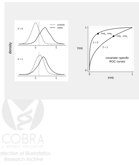
Covariates such as disease severity and specimen storage time can do more than impact marker observations among controls. They often also impact the inherent discriminatory accuracy of the marker (i.e. the ROC curve). That is, they affect the separation between the case and control marker distributions. A hypothetical example is shown in Figure 4. The data can be downloaded from the DABS website. Observe that the separation between the case and control marker distributions is much greater when Z = 0 than when Z = 1. The covariate also affects the distribution of the marker among controls, necessitating covariate adjustment.

ROC regression is a methodology that models the marker’s ROC curve as a function of covariates (Pepe, 2000; Alonzo and Pepe, 2002). Implementation proceeds in two steps: 1) model the distribution of the marker among controls as a function of covariates. Calculate the case percentile values, and; 2) model their CDF (i.e. the ROC curve) as a function of covariates. The result is an estimate of the ROC curve for the marker as a function of covariates, i.e. a covariate-specific ROC curve. We emphasize that the covariates used in step (1) for adjustment are those that affect the marker distribution in the control population; these may or may not differ from the covariates that impact the separation between cases and

(13)

controls, used in step (2).

3.2 Estimation

Estimation of the control marker distribution as a function of covariates and calculation of the case per-centile values proceeds in exactly the same manner as with the covariate adjustment method. The stan-dardization options allowed byrocregare the same as withroccurveandcomproc. The covariates may be assumed to act linearly on marker observations, or stratification can be employed if they are discrete. The percentile values can be calculated by estimating the control marker distribution conditional on covariates empirically or by assuming a normal model.

Next, a parametric model is specified for the ROC curve (ie the CDF of the case percentile values) as a function of covariates. The forms allowed by the rocreg program are

ROCZ(f) = P(1−pvDZ ≤f) =g(α0+α1g−1(f) +α2Z+α3Z×g−1(f)),

where g(·) is the standard normal CDF or the logistic function. The parameter α2 allows the covariates

to impact the “intercept” of the ROC curve, while α3 allows Z to impact the “slope” of the ROC curve.

If α3 6= 0, the covariates have a different impact on the ROC curve at different FPRs. Observe that this

ROC model gives rise to binormal (Dorfman and Alf, 1969) or bilogistic (Ogilvie and Creelman, 1968) ROC curves at each fixed value of Z.

In order to fit the ROC regression model, a discrete set of FPR points, f1, . . . , fnp is chosen. These

points may span (0,1) or a subinterval of interest, (a, b). For each case observation, a set of np records is

created. Thekth_{record includes the binary outcome}_U

ki = I[1−cpvDZi ≤fk] and covariates: g

−1₍_f

k),Z, and Z×g−1₍_f

k). A binary regression model with link g, outcomeU, and covariates: g−1(f),Z, and Z×g−1(f)

provides estimates of (α0, α1, α2, α3) (Alonzo and Pepe, 2002). Bootstrapping is used for inference, where

the data are resampled according to the design.

For illustration, an ROC regression model was fit for DPOAE using the audiology data. DPOAE observations among controls are assumed to depend linearly on age and gender, and their distribution is

(14)

estimated empirically. Age-specific ROC curves are modelled parametrically using

ROCZ(f) = Φ(α0+α1Φ−1(f) +α2Zage). (3)

Estimates of the age-specific ROC curves are calculated using the parameter estimates (αb0,αb1,αb2). Figure

5 shows estimated binormal ROC curves for children at 30, 40, and 50 months of age. This figure suggests that the marker is more accurate among older children, but the effect is not statistically significant (see below).

3.3 The

rocreg

Command

3.3.1 Syntax

The syntax of the rocreg command is

rocreg disease var test varlist [if] [in] [, options]

where disease var is the binary outcome andtest varlist is the list of markers.

3.3.2 Options

Marker Standardization

The options for marker standardization are the same as with roccurve and comproc. Covariates may or may not be used for adjustment.

ROC Regression

The optionregcov(varlist) specifies the list of covariates that have the same impact on the ROC curve at all FPRs. sregcov(varlist) specifies covariates that impact the ROC curve differently at different FPRs.

ROC Calculation

The option linkgoverns whether the model assumes a binormal or bilogistic ROC curve at each value of

Z. Theinterval(a b np) option can be used to specify that the model is fit atnp points over the restricted

FPR interval (a, b).

Sampling Variability

(15)

outcome. Bootstrap sampling options are as with roccurve.

3.4 Example

The rocreg command applied to the audiology data produced the following results:

. rocreg d y1, adjcov(currage gender) adjm(linear) regcov(currage) cl(id) noccsamp ROC regression for markers: DPOAE 65 at 2kHz

model intercept term covariates: currage percentile value calculation

method: empirical tie correction: no Covariate adjustment for p.v. calculation:

method: linear model covariates: currage

Gender GLM fit of binormal curve

number of points: 10 on FPR interval: (0,1)

link function: probit

model coefficient bootstrap se’s and CI’s based on sampling w/o respect to case/control status

number of bootstrap samples: 1000 ******************************

model results for marker: DPOAE 65 at 2kHz

covariate adjustment - linear model, controls only

---+--- F( 2, 4904) = 20.13

Model | 2418.56541 2 1209.2827 Prob > F = 0.0000

---+--- Adj R-squared = 0.0077

Total | 297080.929 4906 60.5546125 Root MSE = 7.7515

---+---currage | -.2032456 .0323905 -6.27 0.000 -.2667455 -.1397458 gender | .2471744 .2229119 1.11 0.268 -.1898327 .6841815 _cons | -1.486659 1.288611 -1.15 0.249 -4.012913 1.039596 ---************ ROC-GLM model

Bootstrap results Number of obs = .

Replications = 1000

---+---alpha_0 | -1.2725052 -.0190699 1.175404 -3.576255 1.031244 (N) | -3.673484 1.027063 (P) | -3.623841 1.037872 (BC) alpha_1 | .93723935 .0144148 .07124306 .7976055 1.076873 (N) | .8213393 1.101304 (P) | .8021784 1.076336 (BC)

(16)

currage | .04482277 .0005192 .03057069 -.0150947 .1047402 (N)

| -.0127396 .1081691 (P)

| -.012525 .1081691 (BC)

4 Evaluating Incremental Value

4.1 Motivation and Concept

Another way of incorporating covariate information is by evaluating incremental value. When Z is a set of known risk factors or other baseline predictors, an obvious question concerns the improvement in classification accuracy associated with adding Y to Z. Note that within this framework, Z is allowed to help in discriminating between cases and controls. This is in contrast to covariate adjustment methods which characterize the classification accuracy of Y conditional on Z.

Incremental value is quantified by comparing the ROC curve for (Y, Z) to the ROC curve for Z alone. The optimal combination of Y and Z for classification is the risk score, P(D = 1|Y, Z) (McIntosh and Pepe, 2002). The risk score can be estimated using a wide variety of binary regression techniques, including logistic regression, logic regression, classification trees, neural networks, and support vector machines.

4.2 Estimation

We propose the following approach to estimating incremental value. First, we fit logistic regression models with and without the marker, Y:

P(D= 1|Y, Z) = g(β0+β1Y +β2Z+β3Z×Y)

and

P(D= 1|Z) = g(γ0+γ1Z),

where g(·) =exp(·)/(1 +exp(·)) is the logistic function. Forms other than linear can be employed for the predictors (eg splines), and interactions may or may not be included. The primary advantage of using

(17)

logistic regression is that the linear predictors, g−1₍_P₍_D_{= 1}_|_{Y, Z}_{)) and}_g−1₍_P₍_D _{= 1}_|_Z_{)), which have the}

same ROC curves as the risk scores, are consistently estimated (up to constants) with case-control data (Prentice and Pyke, 1979).

Having fit the two regression models, we next calculate the associated predicted values for all subjects in the dataset. We analyze the predicted values on the linear predictor scale where distributional assumptions are more easily verified, and again note that the ROC curves for g−1₍_P₍_D _{= 1)) and} _P₍_D _{= 1) are the}

same.

The final step is to plot and compare the ROC curves for the linear predictions from the two models. This can be accomplished using the programs roccurve and comproc.

This procedure is simplistic in at least two respects. First, fitting and evaluating models on the same data is known to produce overly optimistic estimates of model performance. Cross-validation could be used to correct for this overoptimism. Second, the bootstrapping implemented in roccurve and comproc

conditions on the fitted regression models. This accounts for uncertainty in the ROC estimates, but not in the predicted values. Bootstrapping the entire process, from sampling to risk score estimation to ROC estimation, would be desirable. For simplicity, we ignore these issues here, but plan to implement a Stata program that incorporates cross-validation and bootstrapping of the model fitting process in the near future.

4.3 Example

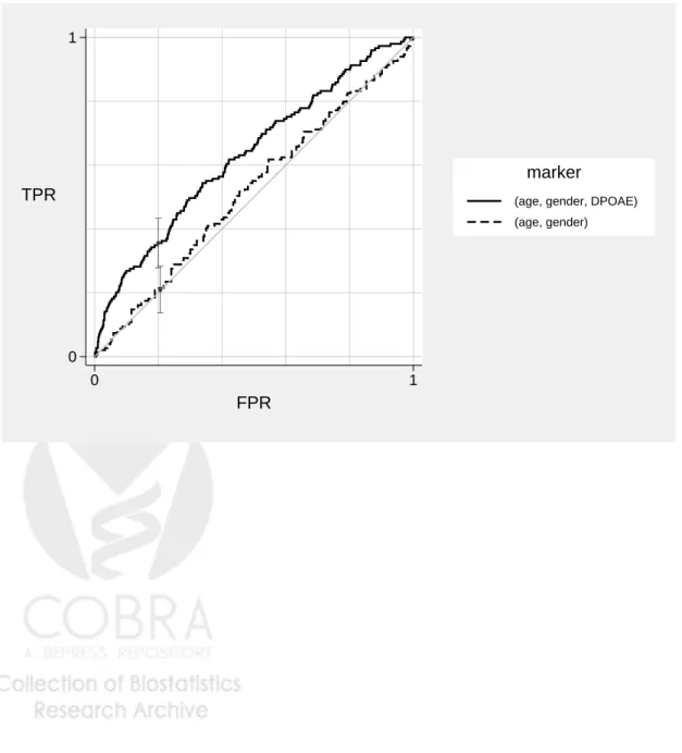
We again use the audiology data to illustrate estimation of incremental value. We evaluate the incremental value of the marker DPOAE over and above age and gender. Figure 6 shows ROC curves for two fitted logistic regression models, one including age and gender, and the other including age, gender, and DPOAE. All covariates are modelled linearly. The ROC curves are estimated empirically (without adjustment for any covariates). We see that DPOAE substantially improves the ability of age and gender to discriminate between hearing impaired and unimpaired ears. The commands used to generate the results are:

logit d currage gender predict p1

(18)

predict p2

roccurve d p1 p2, cl(id) noccsamp

5 Remarks

The methods and Stata programs presented here facilitate incorporating covariates into ROC analysis in three distinct ways: by characterizing the performance of the marker conditional on covariates (ie covariate adjustment), by allowing the accuracy of the marker to depend on the covariates (using ROC regression), and by examining the improvement in classification accuracy associated with adding the marker to the covariates (incremental value). The representation of the ROC curve as the CDF of standardized case marker observations provides a natural means of incorporating covariate information, and gives rise to parametric, semi-parametric, and non-parametric estimates of the quantities of interest.

We have focused on continuous markers but these methods can also be applied to ordinal markers.

References

1. Alonzo TA, Pepe MS. Distribution-free ROC analysis using binary regression techniques. Biostatistics 2002;3:421–32.

2. Baker S. The central role of receiver operating characteristic (ROC) curves in evaluating tests for the early detection of cancer. Journal of the National Cancer Institute 2003;95:511–15.

3. Dodd L, Pepe MS. Partial AUC estimation and regression. Biometrics 2003;59:614–23.

4. Dorfman DD, Alf E. Maximum likelihood esitmation of parameters of signal detection theory and determination of confidence intervals-rating method data. Journal of Mathematical Psychology 1969; 6:487–96.

5. Heagerty P, Pepe MS. Semi-parametric estimation of regression quantiles with application to stan-dardizing weight for height and age in US children. Applied Statistics 1999;48:533–51.

(19)

6. Janes H, Pepe M. Adjusting for covariate effects on classification accuracy using the covariate-adjusted ROC curve. Technical Report 283, UW Biostatistics Working Paper Series, 2006. Available at: http://www.bepress.com/uwbiostat/paper283.

7. Janes H, Pepe M. Adjusting for covariate effects in studies of diagnostic, screening, or prognostic markers: An old concept in a new setting. Technical Report 310, UW Biostatistics Working Paper Series, 2007. Available at: http://www.bepress.com/uwbiostat/paper310.

8. McIntosh M, Pepe M. Combining several screening tests: Optimality of the risk score. Biometrics 2002;58:657–64.

9. Norton SJ, Gorga MP, Widen JE, et al. Identification of neonatal hearing impairment: Evaluation of transient evoked otoacoustic emission, distortion product otoacoustic emission, and auditory brain stem response test performance. Ear and Hearing 2000;21:508–28.

10. Ogilvie JC, Creelman CD. Maximum-likelihood estimation of receiver operating characteristic curve parameters. Journal of Mathematical Psychology 1968;5:377–91.

11. Pepe M. An interpretation for the ROC curve and inference using GLM procedures. Biometrics 2000; 56:352–9.

12. Pepe MS, Cai T. The analysis of placement values for evaluating discriminatory measures. Biometrics 2004;60:528–35.

13. Pepe M, Longton G. Standardizing diagnostic markers to evaluate and compare their performance. Epidemiology 2005;16:598–603.

14. Pepe MS, Longton G, Janes H. Estimation and comparison of receiver operating characteristic curves. Stata Journal 2007;:submitted.

15. Pepe MS, Etzioni R, Feng Z, et al. Phases of biomarker development for early detection of cancer. Journal of the National Cancer Institute 2001;93:1054–61.

16. Prentice RL, Pyke R. Logistic disease incidence models and case-control studies. Biometrika 1979; 66:403–11.

(20)

Figure 1: A simulated marker Y and binary covariate Z = 0,1. Under scenario 1, Z is associated with the outcome: P[D= 1|Z = 0] = 0.36 and P[D = 1|Z = 1] = 0.83. Under scenario 2, Z is independent of the outcome: P[D = 1|Z = 0] = P[D = 1|Z = 1] = 0.50. (a) The densities of Y conditional on Z = 0, conditional on Z = 1, in the pooled data under scenario 1, and in the pooled data under scenario 2. A common threshold is indicated. (b) The common covariate-specific ROC curve, the pooled ROC curve under scenario 1, and the pooled ROC curve under scenario 2. The performances of the common threshold rule are indicated.

−5 0 5 10 controls cases Z = 0 −5 0 5 10 Z = 1 P(D=1) = .50 −5 0 5 10

pooled data scenario 1

P(D=1) = .50

−5 0 5 10

pooled data scenario 2

density (a) 0 1 TPR 0 1 FPR covariate specific pooled, scenario 1 pooled, scenario 2 ROC curves (b)

(21)

Figure 2: Three different estimates of the age- and gender-adjusted ROC curve for DPOAE based on the Norton et al. (2002) audiology data.

0 1 TPR 0 1 FPR empirical pv empirical ROC 0 1 TPR 0 1 FPR normal pv empirical ROC 0 1 TPR 0 1 FPR normal pv binormal ROC DPOAE marker

(22)

Figure 3: Age- and gender-adjusted ROC curves for DPOAE and TEOAE based on the Norton et al. (2002) audiology data. 0 1 TPR 0 1 FPR DPOAE 65 at 2kHz TEOAE 80 at 2kHz marker

(23)

Figure 4: A simulated markerY and binary covariate Z = 0,1. The marker is more accurate whenZ = 0 than when Z = 1, and marker observations among controls also depend on Z. The performances of a common threshold are indicated.

0 5 controls cases Z = 0 0 5 Z = 1 density TPR , FPR 0 0 TPR , FPR 1 1 Z = 0 Z = 1 covariate−specific ROC curves 0 1 TPR 0 1 FPR

(24)

Figure 5: Age-specific ROC curves for DPOAE based on the Norton et al. (2002) audiology data. The ROC curves are adjusted for age and gender.

0 1 TPR 0 1 FPR 30 40 50 Age (months)

(25)

Figure 6: The incremental value of DPOAE over and above age and gender, estimated using the Norton et al. (2002) audiology data. ROC curves are estimated for disease risk prediction models with and without DPOAE. Both models include age and gender.

0 1

TPR

0 1

FPR

(age, gender, DPOAE) (age, gender)