Data Mining Techniques for Complex User-Generated Data

(1)

Porto Institutional Repository

[Doctoral thesis] Data Mining Techniques for Complex User-Generated Data

Original Citation:

Xiao, Xin (2016). Data Mining Techniques for Complex User-Generated Data.PhD thesis

Availability:

This version is available at :http://porto.polito.it/2644046/since: June 2016

Published version:

DOI:10.6092/polito/porto/2644046 Terms of use:

Porto, the institutional repository of the Politecnico di Torino, is provided by the University Library and the IT-Services. The aim is to enable open access to all the world. Pleaseshare with ushow this access benefits you. Your story matters.

(2)

COMPUTER AND CONTROL ENGINEERING XXVIII CYCLE

PhD Thesis

Data Mining Techniques for Complex

User-Generated Data

Supervisor:

Prof. Silvia Chiusano

Author: Xin Xiao Matr. 199914

(3)

Abstract

Computer and Control Engineering XXVIII Cycle

PhD

Data Mining Techniques for Complex User-Generated Data

by Xin Xiao Matr. 199914

Nowadays, the amount of collected information is continuously growing in a variety of different domains. Data mining techniques are powerful instruments to effectively analyze these large data collections and extract hidden and useful knowledge.

Vast amount of User-Generated Data (UGD) is being created every day, such as user behavior, user-generated content, user exploitation of available services and user mobility in different domains. Some common critical issues arise for the UGD analysis process such as the large dataset cardinality and dimensionality, the variable data distribution and inherent sparseness, and the heterogeneous data to model the different facets of the targeted domain. Consequently, the extraction of useful knowledge from such data collections is a challenging task, and proper data mining solutions should be devised for the problem under analysis.

In this thesis work, we focus on the design and development of innovative solutions to support data mining activities over User-Generated Data characterised by different critical issues, via the integration of different data mining techniques in a unified frame-work. Real datasets coming from three example domains characterized by the above critical issues are considered as reference cases, i.e., health care, social network, and ur-ban environment domains. Experimental results show the effectiveness of the proposed approaches to discover useful knowledge from different domains.

(4)

First and foremost, I would like to express my deepest gratitude to my supervisor, Prof. Silvia Chiusano, for her important suggestions and encouragement throughout my PhD course, and for all the opportunities to participate in the research activities in data mining. I’m extremely grateful for the great effort and support she put into training me. Her excellent guidance is extremely precious for my PhD study as well as future career, I hope I could be as enthusiastic and energetic as her in my work.

I would also like to express my great appreciation to Tania Cerquitelli, for her valu-able suggestions and support in most of my research work, as well as offering me the opportunity of teaching activity.

In addition, I would like to thank all my research group colleagues, Prof. Elena Baralis, Luca Cagliero, Paolo Garza, and Giulia Bruno for their support and suggestions at times, especially Paolo who gave me advices during some experiments. Thank also the other group members, it’s my pleasure to work with these nice people. I would also like to thank all the people I met during my PhD study.

I especially thank my parents and all the other family members. They were always supporting me and encouraging me with their best wishes, in the distant home.

Finally, a very special thank to Tao Su, my future husband, for his love, company, care and encouragement throughout all these years abroad.

(5)

Abstract i

Acknowledgements ii

List of Figures v

List of Tables vii

1 Introduction 1

2 Analysis of sparse, high-dimensional data 5

2.1 Analysis of patient treatments. . . 7

2.1.1 Related work . . . 8

2.1.2 Data preparation . . . 9

2.1.3 Multiple-level cluster analysis . . . 12

2.1.4 Cluster evaluation based on quality indices . . . 15

2.1.5 Cluster characterization based on exam frequency and sequential patterns . . . 17

2.1.6 Classification model and mobile application . . . 18

2.1.7 Experimental results . . . 21

2.1.8 Discussion. . . 29

2.2 Analysis of User-Generated Content from Twitter . . . 34

2.2.2 Data collection and preprocessing. . . 37

2.2.3 Cluster analysis. . . 38

2.2.4 Cluster evaluation . . . 38

2.3 Analysis of patient transfers in hospital admissions . . . 44

2.3.2 Data collection and preparation. . . 47

2.3.3 Analysis of intra- and inter-area patient flows . . . 48

2.3.4 Association analysis . . . 49

3 Analysis of heterogeneous data with large cardinality 61 3.1 Analysis of patient treatments with patient profile information . . . 64

(6)

3.1.2 Patient representation . . . 65

3.1.3 Patient clustering through a new distance measure . . . 65

3.1.4 Patient classification . . . 67

3.2 Analysis of User-Generated Content from Twitter with spatio-temporal information . . . 72

3.2.2 Twitter data preparation . . . 75

3.2.3 Clustering analysis through a new distance measure . . . 78

3.2.4 Cluster content characterization . . . 80

3.3 Analysis of air pollution data . . . 91

3.3.2 Data collection and representation . . . 92

3.3.3 Data analysis through generalised association rules . . . 96

4 Analysis of historical data 102 4.1 Analysis of patient physiological data. . . 104

4.1.1 Data collection and preprocessing. . . 106

4.1.2 Prediction analysis . . . 108

4.2 Analysis of User-Generated Data in bike-sharing systems. . . 114

4.2.1 Data collection and preparation. . . 116

4.2.2 Data modeling . . . 117

4.2.3 Station occupancy prediction . . . 120

4.2.4 System exploitation . . . 122

(7)

1.1 User-Generated Data in the research work . . . 2

2.1 Considered sparse, high-dimensional data analysis . . . 5

2.2 _Multiplel-_Level _Data_Analysis framework . . . 6

2.3 The _MLDA framework on treatments of diabetic patients . . . 8

2.4 Mobile app: (a) patient registration, (b) insertion of a new examination done by the patient, (c) visualize patient examination history, (d) patient classification. . . 21

2.5 K-means methods: quality of the cluster set when varying the number of clusters . . . 24

2.6 K-medoids methods: quality of the cluster set when varying the number of clusters . . . 25

2.7 DBSCAN algorithm: quality of the cluster set and number of outlier patients when varying the Epsvalue (M inP ts=30) . . . 26

2.8 Silhouette plot for multiple-level DBSCAN. . . 27

2.9 Refined K-means on the three datasets: quality of the cluster set when varying the number of clusters . . . 29

2.10 Two simplified example tweets . . . 35

2.11 The proposed multiple-level clustering framework for tweet analysis. . . . 36

2.12 Framework to support the lean reorganization of hospitals . . . 46

2.13 Distribution of hospital admissions in the functional areas . . . 54

3.1 Heterogeneous data analysis . . . 62

3.2 Heterogeneous data analysis . . . 63

3.3 Portion of the classification tree . . . 72

3.4 The proposed architecture . . . 74

3.5 Distribution of number of tweets in the cluster set . . . 85

3.6 Spatial characterization of the cluster set . . . 86

3.7 Temporal characterization of the cluster set . . . 86

3.8 Cluster located in the Greater London county: distribution of the number of tweets w.r.t. the top ten counties . . . 87

3.9 Cluster located in the Greater London county: distribution of the number of tweets w.r.t. hourly time frame . . . 87

3.10 Cluster quality by varyingK for TW1_UK (ps= 3, pt= 6) . . . 91

4.1 Historical data analysis . . . 102

4.2 Historical data analysis framework . . . 104

4.3 The _CRPframework . . . 106

4.4 multiple-test model forHRpeak and V O2peak prediction. . . 113

(8)

4.5 V O2next prediction using SVM and ANN. . . 114

4.6 The STation Occupancy Predictor architecture. . . 116

4.7 Effect of the STOP system parameters (Apr-May). . . 128

(9)

2.1 Example of a collection of patient records . . . 9

2.2 VSM representation for dataset in Table 2.1 . . . 10

2.3 VSM representation using the TF-IDF weighting score for dataset in Ta-ble 2.1 . . . 10

2.4 Comparison of multiple-level clustering algorithms . . . 14

2.5 Most frequent examinations for each category in the diabetes dataset . . . 22

2.6 Detailed clustering results for refined K-means . . . 25

2.7 Clustering results for multiple-level DBSCAN . . . 26

2.8 Detailed clustering results for multiple-level DBSCAN . . . 27

2.9 Clustering results for multiple-level DBSCAN on datasets with 30 and 60 examinations . . . 29

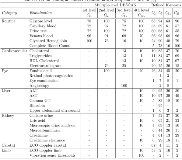
2.10 Multiple-level DBSCAN and refined K-means: most frequent examina-tions in some example clusters (examination frequencies are in %) . . . . 32

2.11 Example of maximal sequential patterns for some clusters from multiple-level DBSCAN . . . 33

2.12 First- and second-level clusters in the paralympics dataset (DBSCAN parametersM inP ts=30,Eps=0.39 andM inP ts=25,Eps=0.49 for first-and second-level iterations, respectively) . . . 43

2.13 First- and second- level clusters in the concert dataset (DBSCAN param-eters M inP ts=40, Eps=0.41 and M inP ts=21, Eps=0.62 for the first-and second-level iterations, respectively) . . . 44

2.14 Functional areas and corresponding wards . . . 48

2.15 Example of hospital admission dataset . . . 48

2.16 Transactional format of hospital admission data. . . 50

2.17 Sequential format of hospital admission data . . . 51

2.18 Intra-area association rules . . . 56

2.19 Support and confidence of inter-area association rules (2007 - 2013). . . . 59

2.20 Example of intra-area Sequential rules . . . 59

3.1 Patient conditions for discovered clusters. . . 69

3.2 Exam frequencies in first level clusters (M inP ts=30,Eps=0.04,wa= 0.3, wg = 0.05,wE = 0.65) . . . 69

3.3 Exam frequencies in second level clusters (M inP ts=25,Eps=0.07, wa= 0.3,wg = 0.05,wE = 0.65) . . . 70

3.4 Tweet example . . . 76

3.5 List of some topics . . . 82

3.6 Main characteristics of dataset partitions . . . 84

3.7 Characterization of five example clusters in Figure 3.5 . . . 87

(10)

3.8 Rules characterizing cluster C extracted from Dataset a1 . . . 89

3.9 Rules characterizing clusters in Datasetsa1,b1, and c1 (rule class WC) . . 90

3.10 Dataset attributes . . . 94

3.11 Discretized humidity values and UV radiations . . . 95

3.12 Example taxonomy . . . 96

3.13 Rule examples. . . 100

4.1 Monitored physiological signals . . . 107

4.2 Characteristics of the dataset. For all signals, mean and standard devia-tion (SD), minimum, and maximum values are reported. . . 111

4.3 Rule types. . . 124

4.4 Prediction quality of STOP in different time periods by using AODEsr and L3. . . 126

(11)

Introduction

Nowadays, the rapid development of online systems or devices have given rise to a huge amount of electronic data. The inexpensive effort for data capturing and storage has enabled huge data generation from various industries and innovations, such as banking, healthcare, social network, e-commerce and urban context. The need to extract useful knowledge from these huge, complex, information-rich data collections is becoming more and more important in the real world.

Data mining techniques are powerful instruments that can be effectively used to ana-lyze these large data collections and extract hidden and useful knowledge. Data mining techniques have been successfully applied in various application domains as telecommu-nications, healthcare, and web. They allow extracting previously unknown interesting patterns such as discovering groups of similar data objects (cluster analysis), mining correlations among data objects (association analysis), building a model describing data classes and assigning a class label to a new unlabeled data object (classification), or predict the future values for continous data (regression).

The research activity carried out in the PhD is on using data mining techniques for data analysis on complex application domains. For these domains, some common critical issues arise for the data analysis process. Data collections can be characterized by a

large cardinalityanddimensionality, avariable data distributionandinherent sparseness. In addition, to model the different facets of the targeted domain heterogeneous data

types should be considered in the data analysis process. Historical data should also be considered to properly characterize the problem under analysis. Consequently, the extraction of useful knowledge from such data collections is a challenging task, and proper data mining solutions should be devised.

(12)

Figure 1.1: User-Generated Data in the research work

In the PhD research activity, three application domains characterized by the above critical issues are considered as reference example case. These domains are the health care domain, the social network domain, and the urban environment.

Particularly relevant for the knowledge extraction process in these domains is the anal-ysis of User-Generated data (UGD). The vast amount of UGD created every day is a significant challenge for data analysis due to the various data types and their common critical issues. The UGD considered in this study for the three reference domains in-cludes data on user behavior, on user exploitation of available services, on user mobility and on user-generated content (see Figure1.1). For example, in the health care domain, data on user behavior refer to the patient history on the underwent treatments. These data can be analysed to extract a variety of information on the medical treatments cur-rently adopted and gain insights for improving medical guidelines for a give disease. In the social network domain, User-Generated Data refer to the content in tweet messages, possibly also including spatio-temporal information on “when” and “where” the tweet has been posted. These data can be analysed to extract various knowledge such as user activities or topics of interest, personal options and user emotions.

This thesis work focuses on design and development of innovative solutions to analyze User-Generated Data (UGD) in complex application domains. Since a single data mining technique may not fit the heterogeneous characteristics of the data under analysis, the research activity addressed the integration of different data mining techniques in a unified framework, as the jointly exploitation of clustering and classification techniques and clustering and association analysis. Real datasets are considered to assess the proposed approaches. More specifically, data mining techniques have been studied and developed in the PhD research to address the following issues.

Analysis of sparse, high-dimensional data with variable distribution. Real-world data collections are usually characterized by an inherent sparseness and variable

(13)

distribution, since they are generated by a large variety of events, and high data di-mensionality because features used to model real objects and human actions may have very large domains. The variability in data distribution grows with data volume, thus increasing the complexity of mining such data. In the research activity, some reference examples of sparse, high-dimensional data coming from the health care and social net-work domains have been considered. For example in health care domain, because of the variety of medical treatments usually adopted for the different degrees of severity of a given pathology, patient data collections are usually characterized by inherent sparse-ness, high dimensionality and variable distribution. To deal with these issues, in the research activity a unified framework named Multiplel-Level Data Analysis (MLDA) framework has been proposed, by jointly exploiting multiple-level clustering, association, and classification analysis.

Analysis of heterogeneous data with large cardinality. Heterogeneous data is a common characteristic of datasets in various domains to model data under different facets. Failing to take the heterogeneous issue into account can easily derail the discov-eries from these data. In the research activity we considered some reference examples of heterogeneous data coming from the health care, social network and urban environment domains. For example, when analyzing patient treatments in the health care domain, despite patient examinations, patient profile information such as age and gender can be also taken into account. Innovative data analytics solutions able to acquire, integrate and analyze data containing large amount of heterogeneous dimensions are needed. To address the above issues, in the research activity, novel combined distance measures tak-ing into account all considered facets of the problem under analysis have been proposed and integrated into the clustering process. When aimed at discovering interesting corre-lations in the heterogeneous UGD, data taxonomy integrated with association analysis has been also presented to discover correlations among heterogeneous data at different abstraction levels.

Analysis of historical data. Historical data is data collected in past-periods, used usually as a basis for forecasting the future data values or trends. Historical data is often represented as time series records, which has been useful in helping predict the future of a company and a market through predictive analyses. In the research work we considered some reference examples of historical data coming from the health care and urban environment domains. In health care domain, an example of historical UGD is the collection of physiological signal values describing the cardiac and respiratory response of patients during a cardiopulmonary exercise test, where the physiological

(14)

signal values are multivariate time series. Since the test is physically very demanding, innovative data analysis techniques are needed to predict patient response thus lowering body stress and avoiding cardiopulmonary overload. To deal with these issues, in the research activity, a framework has been proposed to predict future values based on historical UGD collected in a time window, by jointly exploiting windowing approach and classification or regression techniques.

This thesis is organized as follows. The analysis of sparse, high-dimensional data with variable distribution is described in Chapter 2. Chapter 3 presents the analysis of heterogeneous data with large cardinality. Chapter 4 describes the extraction of useful knowledge from historical data. Finally, Chapter 5 presents conclusions and discusses future developments for the proposed approaches.

(15)

Analysis of sparse,

high-dimensional data

This chapter describes data mining algorithms designed and developed in this PhD thesis to analyze sparse, high-dimensional User-Generated Data. Real-world data collections are usually characterized by aninherent sparsenessand variable distribution, since they are generated by a large variety of events, andhigh data dimensionalitybecause features used to model real objects and human actions may have very large domains. The variability in data distribution grows with data volume, thus increasing the complexity of mining such data. However, at present, most single data mining algorithms perform better with uniform data distribution, while their performance as well as the quality of the extracted knowledge tend to decrease in non-uniform collections. Consequently, the extraction of useful knowledge from such data collections is a challenging task. It’s necessary to jointly exploit data mining techniques and proper data mining solutions should be devised for the problem under analysis.

In the research activity carried out during the PhD study, some reference examples char-acterized by these issues have been considered coming from the health-care domain and social network domain (see Figure 2.1). In the health care domain, data on treatments

Figure 2.1: Considered sparse, high-dimensional data analysis

(16)

Figure 2.2: Multiplel-LevelDataAnalysis framework

underwent by patients and on patient transfers in hospital admissions have been con-sidered. Health care data collections can have large volume due to the large cardinality of patient records. Because of the variety of medical treatments usually adopted for the different degrees of severity of a given pathology, patient data collections are also usually characterized by high dimensionality, variable data distribution and inherent sparseness. Because of the various wards among which patients may transfer in hospital admission, during the analysis of patient transfers the issues also exist. In social network domain, User Generated Content (UGC) from Twitter messages is also characterised by inherent sparseness, due to the limitation of 140 characters in the message.

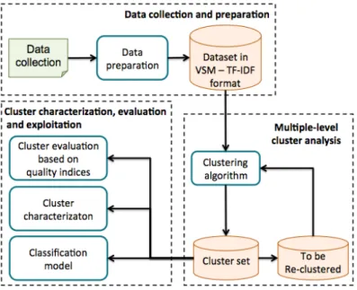
Aimed at addressing the above issues, in the research activity, a unified data anal-ysis framework named _Multiplel-_Level _Data _Analysis (_MLDA) framework, has been proposed, by jointly exploiting multiple-level clustering, association, and classification analysis. The main architecture blocks, depicted in Figure 2.2, are (i) Data collection and preparation, the considered data collection is first prepared and represented in the Vector Space Model (VSM) [1] using the Term Frequency - Inverse Document Frequency (TF-IDF) method [2]. The VSM representation has been applied in previous works [1] to represent text documents, while the TF-IDF scheme has been used to weight the relevance of words appearing in the document. (ii)Multiple-level cluster analysis, where clustering algorithms are exploited in a multiple-level fashion to iteratively focus on different dataset portions andlocally identify groups of correlated objects. It allows dis-covering cohesive and well-separated clusters with divers data distributions. (iii)Cluster characterization, evaluation and exploitation, where the quality of discovered clusters is evaluated based on various indices such as Sum of Squared Error (SSE), Silhouette, and

(17)

Overall Similarity (see Section2.1.4). The cluster content is also concisely characterized through association analysis capturing correlations among data features. Moreover, for supporting the automatic categorization of a new data object into one of the discovered cluster, a classification model can be created starting from the computed cluster set.

In this thesis, the complete instance of the MLDA framework has been exploited to analyse diabetic patient treatments as a reference case study in Section 2.1. Sections 2.2 and 2.3 describe the application of preliminary instances of the _MLDA framework on User-Generated Content in social network and on patient transfers in health-care domains, respectively.

2.1 Analysis of patient treatments

This section describes the exploitation of a complete instance of theMLDA framework to analyze treatments of diabetic patients. A real dataset including the examination log data of (anonymized) patients with overt diabetes has been considered as a reference case study. Diabetes describes a group of metabolic diseases in which the patient has high blood glucose. Diabetic patients may suffer by various disease complications as eye problems, neuropathy, kidney and cardiovascular diseases. Patients affected by disease complications (or at risk of them) should be tested with more specific examinations in addition to routine tests to monitor its status (or reveal the pathology). The work presented in this section has been published in [3].

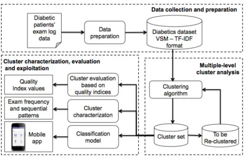
The components of the MLDA framework for patient treatments analysis are depicted in Figure2.3. In thedata preparation phase the collection of diabetic patients’ exam log data is tailored to the Vector Space Model (VSM) representation [1] using the TF-IDF method [2], with the aim of highlighting the relevance of specific data characteristics.

Then, in the data clustering phase prepared data are clustered using a multiple level clustering strategy. In this study, five different multiple-level clustering algorithms have been integrated into_MLDA, based on K-means (i.e., bisecting and refined K-means [4]), K-medoids (i.e., bisecting and refined K-medoids [5]), and DBSCAN methods (i.e., multiple-level DBSCAN [6]). Clustering results have been then analyzed and compared using some well-established quality indices, as SSE, Silhouette and overall similarity, and Rand Index [2].

Finally, in the cluster characterization, evaluation and exploitation phase, the cluster content has been analysed with the aim of providing useful information to the final end-user. For cluster characterization, maximal sequential patterns [7] have been selected to concisely describe temporal correlations among data features appearing in each cluster.

(18)

Figure 2.3: TheMLDAframework on treatments of diabetic patients

A classification model has been built using decision trees [2], which have been shown to provide accurate models in various applications. To allow ubiquitous classification on new data, real-time analysis is executed on mobile devices through an ad-hoc Android application exploiting the classification model.

2.1.1 Related work

In health-care domain, many studies addressed the identification of correlated groups of patients affected by different diseases. For example, [8] reviewed the cluster methods used to diagnose heart valve diseases. In [9], clustering techniques were used to diagnose breast cancer based on tutor features, by recognising hidden patterns of benign and ma-lignant tumors. Authors in [10] exploited the K-means algorithm to cluster a collection of patient records aimed at identifying relevant features of patients subjected to heart attack.

Some research efforts have been devoted to exploiting clustering techniques on data re-lated to diabetic patients [11]. Different issues have been addressed as food analysis [12], gait patterns [13], discovering relationships among diabetes and risk factors [14], anal-yses of various imputation techniques [15], and discovering similar medical treatments [6]. [15] focuses on diabetes datasets using the K-means algorithm aimed at analysing various imputation techniques. Different from [15], in the framework we aim at iden-tifying groups of patients with similar examination histories to provide a preliminar patient categorization into a set of predefined classes. Thus, we detailed each cluster

(19)

with sequential patterns to discover how examinations are interleaved and distributed over time.

The wide diffusion of mobile technologies and the increasing capabilities of mobile com-puting devices caused an increased interest in designing, implementing and testing inno-vative applications running on mobile devices to provide a wide range of useful services based on user-generated data. In the medical care scenario, some efforts [16, 17, 18] have been devoted on this appealing research. In [16], a distributed end-to-end per-vasive healthcare system utilizing neural network computations for diagnosing diabetes was developed in small mobile devices. [17] developed a new mobile-based approach to automatically detect seizures, using k-means as unsupervised classification technique. [18] have presented Generalized Discriminant Analysis and Least Square Support Vector Machine models to diagnose the diabetes disease. Also in this study, we integrated in the framework a two-tier architecture to allows ubiquitous patient classification through a mobile application. The proposed solution allows to efficiently and effectively exploit-ing knowledge items discovered through multiple-level cluster analysis to different user profiles (e.g., medical staff, patients). Thus, the proposed mobile application allows ubiquitous patient classification on new unlabelled examination histories.

2.1.2 Data preparation

The considered data collection is characterized by an inherently sparse distribution due to the variety of possible examinations, covering both routine tests and more specific examinations for different degrees of severity in diabetes. In the considered collection of patient records, each record corresponds to a medical examination done by a patient in a given date. For instance, Table 2.1 shows a toy example dataset listing the medical examinations undergone by two patientsp1andp2in year 2014. A more formal definition

of a collection of patient records is given in Definition 2.1.1.

Table 2.1: Example of a collection of patient records

PatientID Examination Date PatientID Examination Date

p1 Glucose level 2014-02-10 p2 Urine test 2014-12-01

p2 Fundus oculi 2014-01-06 p2 Triglycerides 2014-11-30

p2 Urine test 2014-02-28 p2 Urine test 2013-04-16

p1 Fundus oculi 2014-03-10 p1 Urine test 2014-09-06

p2 Urine test 2014-04-11 p2 Triglycerides 2014-08-01

p₁ Glucose level 2014-04-15 p₂ Urine test 2014-07-25

p2 Electrocardiogram 2014-06-16 p1 Fundus oculi 2014-07-10

p1 Glucose level 2014-06-21 p1 Urine test 2014-11-23

Definition 2.1.1. Collection of patient records. A collection of patient records D

(20)

Table 2.2: VSM representation for dataset in Table2.1

PatientID Glucose level Fundus oculi Electrocardiogram Urine test Triglycerides

p1 3 2 0 2 0

p2 0 1 1 5 2

Table 2.3: VSM representation using the TF-IDF weighting score for dataset in Ta-ble2.1

PatientID Glucose level Fundus oculi Electrocardiogram Urine test Triglycerides

p1 0.347 0 0 0 0

p2 0 0 0.077 0 0.154

Θ ={p1, . . . , pn}is the set of patients inD. Each recordrk inDmodels an examination

ej ∈Σ done by a patient pi ∈Θ in a given date.

To enable the mining process and discover valuable knowledge, in the_MLDAframework the collection of patient records is tailored to the Vector Space Model (VSM) represen-tation [1] and the Term Frequency (TF) - Inverse Document Frequency (IDF) scheme [2] has been adopted to weight the examination frequency. In this study, we neglect the information on when an examination has been done because we focus on the frequency of performed examinations.

In the VSM representation, each patient pi is a vector in the examination space. This vector represents the patient examination history. The vector cell (pi, ej) corresponds to examination ej done by patient pi. Cell (pi, ej) is a weight describing the relevance of examination ej for patient pi. A more formal definition of the patient examination history follows.

Definition 2.1.2. Patient examination history. Let D be a collection of patient records, Σ = {e1, . . . , ek} the set of examinations in D and Θ = {p1, . . . , pn} the set of patients inD. Each patientpi inDis represented by a weighted examination frequency vectorvpi of|Σ|cells. Each cell vpi[j] of vectorvpi reports the weighted frequencywpi,ej of examination ej,ej ∈Σ, for patient pi,pi∈Θ. Thus,vpi = [wpi,e1, . . . , wpi,e|Σ|].

Table 2.2 reports a base VSM representation for the example dataset in Table 2.1. Table 2.2 has one row for each patient in Table 2.1, and a number of columns equal to the number of different examinations in Table 2.1. Each cell (pi, ej) in Table 2.2 reports the weight of examinationej for patientpi. In this base VSM representation the weight is simply given by the number of times examinationejwas repeated by patientpi. However, a patient data representation as in Table 2.2 may not properly characterize the patient condition. In fact, it may give more relevance to standard routine tests, which usually appear with higher frequency, than to more specific tests, which often appear with lower frequency. The adoption of the TF-IDF scheme allows highlighting

(21)

the relevance of specific examinations for a given patient condition. The TF-IDF value increases proportionally to the number of times an examination has been done by the patient, but it is offset by the frequency of the examination in the examination dataset, which helps to control the fact that some examinations are generally more common than others. The definitions of TF and IDF are given below.

Definition2.1.3. Term Frequency (TF) and Inverse Document Frequency (IDF).

LetD be a collection of patient records, Σ ={e1, . . . , ek} the set of examinations inD, and Θ ={p1, . . . , pn} the set of patients inD.

1. For each pair (pi,ej) in D, the Term FrequencyT Fpi,ej is the relative frequency of examinationej for patientpi. It is computed asfpi,ej/

P

1≤k≤|Σ|fpi,ek, wherefpi,ej is the number of times patientpi underwent examinationej andP1≤k≤|Σ|fpi,ek is the total number of examinations done bypi.

Mathematically, the base of the log function for IDF computation in Definition 2.1.3 does not matter and constitutes a constant multiplicative factor towards the overall result.

The TF-IDF weight wpi,ej for the pair (pi, ej) is high when examination ej appears with high frequency in patient pi and low frequency in patients in the collection D. When examinationej appears in more patients, the ratio inside the IDF’s log function approaches 1, and theIDFej value and TF-IDF weightwpi,ej become close to 0. Hence, the approach tends to filter out common examinations. A more formal definition of TF-IDF weight follows.

Definition 2.1.4. TF-IDF weight. For each pair (pi,ej) inD, the TF-IDF weightwpi,ej is computed aswpi,ej =T Fpi,ej∗IDFej, whereT Fpi,ej is the Term Frequency andIDFej is the Inverse Document Frequency.

Table 2.3 reports the VSM representation using the TF-IDF scheme for the example dataset in Table 2.1. The TF-IDF weights for examinations Fondus oculi and Urine Test are equal to 0 since they are performed by both patients. Instead, TF-IDF weights are different than zero for the other examinations, which are performed by only one of the two patients.

(22)

2.1.3 Multiple-level cluster analysis

The _MLDAframework applies clustering algorithms in a multiple-level fashion to pro-gressively focus on different dataset portions and locally compute clusters. The pseu-docode of the multiple-level clustering strategy is in Algorithm 1. It performs multiple runs over the considered data collection. Initially, the whole dataset is analysed. Then, at each subsequent iteration, the clustering algorithm is applied on a selected portion of the dataset, and clusters are locally identified on it. Clustering algorithm param-eters can be properly set at each iteration according to the local data distribution of the considered dataset portion. Clusters computed at each iteration contribute to the final cluster set. The approach is iterated until the target objective is achieved, as the minimum threshold value of a given quality index or the maximum allowed number of clusters in the final cluster set.

Data: Initialize Dwith the whole initial data object collection

repeat

if first iteration then

select Das target dataset;

else

select a portion of Das target dataset;

end

apply basic clustering algorithm on the target dataset; update the final cluster set;

evaluate the quality of the final cluster set;

until target objective is verified;

Algorithm 1: Multiple-level clustering strategy

Clustering algorithms currently integrated in _MLDA are described in Section 2.1.3.1. Data objects in the analysed data collection corresponds to patients in our application scenario. For patient clustering, patient examination histories are compared using the cosine distance measure (see Section 2.1.3.2).

2.1.3.1 Multiple-level clustering algorithms

Clustering algorithms integrated in theMLDAframework are described in the following. Their main characteristics are summarized in Table2.4, by highlighting the improvement with respect to the corresponding (not multiple-level) standard algorithms. Based on this evaluation, they appear as good candidates for the analysis considered in this study. Objects in the analyzed data collection correspond to patients in our application scenario.

Bisecting K-means [4] applies the standard K-means algorithm in a multiple-level fashion. K-means [19] discovers K clusters modeled by their representatives, named

(23)

centroids, given by the mean value of the objects in the clusters. Initially, K objects of the dataset are randomly chosen as centroids. Then, each object is assigned to the cluster whose centroid is the nearest to that object. Finally, centroids are relocated by computing the mean of the objects within each cluster. The process iterates until centroids do not change or some objective functions are achieved.

Nevertheless K-means is a widely used clustering method, it is biased to spherical clusters and it is sensitive to the initial choice of centroids. Aimed at overcoming this second limitation, the bisecting K-means algorithm adopts a multiple-level clustering approach based on a bisecting strategy. Instead of looking for all representative centroids (and corresponding clusters) at the same time, it iteratively focuses on a dataset portion and locally identifies centroids (and their clusters). More in detail, two clusters are initially generated using the standard K-means algorithm. Then, at each subsequent iteration level, a cluster is selected among those generated up to the current step. The selected cluster is split into two subclusters using K-means. K-1 level iterations are needed for discovering the desired K clusters. Different criteria can be exploited to choose the cluster to split: (i) The cluster size (i.e., the number of objects in the cluster), (ii) the cluster SSE (Sum of Squared Errors), which measures the squared total distances among cluster objects and cluster centroid, and (iii) a criterion based on both cluster size and SSE. In this study, the cluster with the largest SSE value is split.

Bisecting K-medoids [5] relies on the standard K-medoid algorithm (PAM) [20] for implementing a multiple-level clustering technique similar to bisecting means. K-medoid works similarly to K-means, but clusters are in this case represented by an object (medoid) instead of a mean point (centroid). As for bisecting K-means, bisecting K-medoids is less susceptible to the initialization problems than standard K-medoids. K-medoids methods were also investigated in this study, since they can be less sensitive to outliers than K-means methods.

Refined K-means and refined K-medoids[4]. Both bisecting strategies described above use the standard (K-means and K-medoids) clustering algorithms to bisect indi-vidual clusters. It follows that the final cluster set does not represent a local minimum with respect to the total SSE value over the whole cluster set. To deal with this problem, the cluster set generated by bisecting K-means and bisecting K-medoids can be refined as follows. The centroids (resp. medoids) in the computed cluster set are used as the initial centroids (resp. medoids) for the standard K-means (resp. K-medoids) algorithm.

Multiple-Level DBSCAN[6] progressively applies the standard DBSCAN [21] algo-rithm on different (disjoint) dataset portions. DBSCAN separates dense regions (with a

(24)

Table 2.4: Comparison of multiple-level clustering algorithms

Bisecting and Refined Bisecting and Refined Multiple-level

K-means K-medoids DBSCAN

Initialization problem Reduced Reduced No

Sensitivity to outliers Reduced Reduced No

Unclustered data objects No No Reduced

Need of convex shape Yes Yes No

Parameter specification K K Eps, MinPts

Num. of iterations

Num. of iterations K-1 K-1 To be specified

Dealing with variable Improved Improved Improved

data distribution

similar density) from a sparse one in the dataset, driven by the user-specified parameters

Epsand MinPts. A dense region in the data space is a n-dimensional sphere with radius

Eps and containing at least MinPts objects. Objects are classified as being (i) in the interior of a dense region (a core point), (ii) on the edge of a dense region (a border point), or (iii) in a sparsely occupied region (an outlier point). A cluster contains any two core points close within a distanceEps, and any border point close within a distance

Eps to at least one core point in the cluster. Outlier points are filtered out and they are unclustered.

Standard DBSCAN can discover clusters with different sizes and shapes, but it is weak in recognizing clusters with variant density. The multiple-level DBSCAN algorithm al-lows overcoming this limitation, by decomposing the clustering process into subsequent steps. The whole original dataset is clustered at the first level. Then, at each subse-quent level, objects labeled as outliers in the previous level are re-clustered using the standard DBSCAN. With the multiple-level approach, parametersEps andMinPts can be set at each level by adapting the definition of dense region to the local data density. Furthermore, the number of unclustered outlier points progressively reduces at each it-eration level. Consequently, the multiple-level DBSCAN algorithm can finally provide a more homogenous but also richer cluster set, because it includes a larger portion of the original dataset. The number of iteration levels can be tuned based on the final number of unclustered objects and the number of computed clusters.

2.1.3.2 Comparing patient examination histories

For all clustering algorithms described above, the weighted examination frequency vec-tors representing the patient examination histories are compared using the cosine dis-tance measure [2]. In our reference case study, letpi andpj be two arbitrary patients in the collection D. Letvpi and vpj be the corresponding weighted examination frequency vectors. The cosine distance between patientspi and pj is computed as

(25)

dist(pi, pj) = arccos (cos(vpi, vpj)) (2.1)

where the cosine similarity between patientspi and pj is computed as

cos(vpi, vpj) = vpi•vpj kvpik vpj = P 1≤k≤|Σ|vpi[k]vpj[k] q P 1≤k≤|Σ|vpi[k]2 q P 1≤k≤|Σ|vpj[k]2 . (2.2)

The cosine distance in Equation2.1verifies the triangle inequality. The cosine similarity is in the range [0,1]. cos(vpi, vpj) equal to 1 describes the exact similarity of examination histories for patients pi and pj, while cos(vpi, vpj) equal to 0 points out that patients have complementary histories (i.e., the sets of their examinations are disjoint).

2.1.4 Cluster evaluation based on quality indices

For the (internal) validation of clustering results, _MLDA adopts the quality indices typically used for the considered algorithms. The Total SSE index [2] is used for K-means and K-medoids methods, while the Silhouette coefficient [22] for the multiple-level DBSCAN approach. Similar to [4], the overall similarity measure is used to compare cluster sets computed by different algorithms. Finally, the Rand Index [23] has been used to evaluate the agreement between different clustering results.

TheSum of Squared Error (SSE)is used to evaluate the cluster cohesion for center-based clusters, as clusters generated using K-means and K-medoids methods [2]. For an arbitrary patient, its error is computed as the squared distance between the patient and the centroid (resp. medoid) in the cluster including the patient. The SSE for a cluster Ci is computed as

SSE(Ci) =

X

pj∈Ci

dist(ci, pj)2 (2.3)

where dist(ci, pj) is the distance between the centroid (resp. medoid) ci of cluster Ci and a patient pj in Ci. The cosine distance metric in Equation 2.1 has been used for distance evaluation. The smaller the SSE, the better the quality of the cluster. The

Total SSE on a set of K clusters is computed by summing up the SSE values of the K clusters.

TheSilhouetteindex measures both intra-cluster cohesion and inter-cluster separation to evaluate the appropriateness of the assignment of a data object to a cluster rather

(26)

than to another one [22]. The silhouette value for a given patient pi in a cluster C is computed as s(pi) = b(pi)−a(pi) max{a(pi), b(pi)} , s(pi)∈[−1,1], (2.4)

where a(pi) is the average distance of patient pi from all other patients in cluster C, andb(pi) is the smallest of average distances from its neighbour clusters. The silhouette value for clusterC is the average silhouette value on all patients inC. Silhouette values in the range [0.51,0.70] and [0.71,1] show that a reasonable and a strong cluster structure has been found [20]. Lower silhouette values progressively indicate clusters with a weak structure until a no substantial structure. The cosine distance metric in Equation 2.1 has been used for silhouette evaluation.

The Overall Similarityindex evaluates the cluster quality. In this study, it has been adopted for comparing the cluster sets from the algorithms integrated into the _MLDA framework. Specifically, it is used to measure the cluster cohesiveness based on the pairwise cosine similarity of patients in a cluster. For each clusterC, the overall similarity is computed as Overall_Similarity(C) = 1 |C|2 X vpi∈C vpj∈C cos(vpi, vpj) (2.5)

where |C|is the cluster size, cos(vpi, vpj) is the cosine similarity between two patients

pi and pj inC represented by their weighted examination frequency vectorsvpi andvpj. The overall similarity on a set of K clusters is computed as the weighted similarity of the clusters Overall Similarity = K X i=1 |Ci| N Overall_Similarity(Ci) (2.6) where N is the total number of patients in the cluster set.

TheRand Indexcomputes the number of pairwise agreements between two partitions of a set [23]. It is exploited to measure the similarity between the cluster sets obtained by two different clustering techniques. In our case study, let O be a set of N patients, and X and Y two different partitions of set O to be compared. The Rand Index R is computed as

(27)

R= a_N+b

2

(2.7)

whereadenotes the number of pairs of patients inO which are in the same cluster both in X and Y, and b denotes the number of pairs of patients in O which do not belong to the same cluster neither in X nor in Y . Therefore, the term a+b is the number of pair wise agreements ofX andY, while N₂

is the number of different pairs of elements which can be extracted fromO. The Rand Index ranges from 0 to 1, where 0 indicates that the two partitions do not agree for any patient pair, and 1 that the two partitions are equivalent.

2.1.5 Cluster characterization based on exam frequency and sequential patterns

In the MLDA framework, the content of each computed cluster is concisely described as follows. (i) The most representative examinations occurring in their patient histo-ries. (ii) The temporal relationship among examinations underwent by patients, i.e., which examinations frequently precede or follow other examinations. This information provides a more detailed characterizion of patient histories because the distribution of patient examinations over time is analysed. The two analyses can support a first cat-egorization of the cluster content into a category of patients (possibly) affected by a given diabetes pathology. In fact, the different pathologies usually require monitoring the patient through some specific examinations.

To support temporal data analysis, the patient data collection contained in each cluster is represented as asequence database[2]. Then, within each cluster, thesequential patterns of medical examination sets underwent by patients in subsequent days are analyzed.

Definition 2.1.5. Sequence database. Let D be a collection of patient records. Let C⊆ D be a cluster onDcontaining a subset of patient records. The sequence database

DS defined on C is a collection of sequences pi:S, where pi is the patient identifier and

S=< s1 . . . sn> is the temporal list of setsst of examinations ej done by pi.

When examinations are done within a short time frame, their temporal order may not be relevant being due to scheduling reasons rather than prescription constraint. For example, in the considered case study of diabetic patients, routine checks through blood tests are usually performed on the same day. Thus, in our data representation, each element st in a sequence pi:S represents the set of examinations done patient pi on the same day.

(28)

The number of elementsstin a sequence S is thesequence length. It corresponds to the number of different days in which the patient has performed at least one examination. The sequence length provides the information on how frequently the patient conditions have been monitored. For example, sequence pi :S =<(e1)(e2,e3)(e4)(e1)> has length

equal to 4 because patientpi performed examinations on 4 different days. The sequence element (e2 e3) includes examinationse2 and e3 done on the same day.

A sequence S is said to contain a sequence S0 if S0 is a subsequence of S, i.e., S0 contains a subset of the elements in S and preserves their order. S is called super-sequence of S0. For example, sequence S0 =<(e3)(e1)> is a subsequence of sequence

S =<(e1)(e2,e3)(e4)(e1)>. Thesupport (or frequency) on the sequence database DS of a sequence S0 is the percentage of sequences in D_S that contain S0. A sequence S0 is a

sequential pattern if its support is above a user-specified minimum support threshold. Mining the complete set of sequential patterns in all discovered clusters may often pro-vide a too large solution set, making difficult for end-users the comprehension of the results. To overcome this limitation, compact representations of the sequential pattern set have been proposed (as closed sequential patterns and maximal sequential patterns). Among them, maximal sequential patterns [7] have been adopted in this study. The set of maximal sequential patterns is representative since it can be used to recover all sequential patterns, and the exact frequency of these latter can also be computed with a single database pass. Besides, the set of maximal sequential patterns is generally a small subset of the set of (closed) sequential patterns. A sequential patternS0 is said to be amaximal sequential pattern if there is no other sequential patternS00 so that S00 is a superpattern ofS0 [7].

2.1.6 Classification model and mobile application

Clusters computed as described in Section2.1.3.1 and characterized as reported in Sec-tion2.1.5can be analyzed with the support of a domain expert to describe their content from a medical perspective and assign a representative class label to each of them. Then, to automatically categorize a new patient into one cluster based on his/her examination history, a classification model can be created starting from the discovered cluster set. The possibility of automatically categorize patient histories using the classification model has been made accessible to end-users through a mobile application (app). The mobile app also allows collecting and updating the user-generated data such as examinations inserted by the patients.

(29)

2.1.6.1 Patient classification model

Classification is the task of learning a classification model that maps each data object to one of the predefined class labels [2]. A classification model is typically used to assign the class label for a new unlabeled data object. Among various classification methods, decision tree classifiers have been used in this study to characterize the results of the clustering process. Decision trees are powerful classification methods that have been widely used in many different application domains. Besides, they provide a readable classification model that can also serve to explain what features characterize objects in each class.

The decision tree is grown in a recursive fashion by iteratively partitioning the training records into successively purer subsets. In the tree structure, each node specifies a test on an attribute, and each branch descending from that node corresponds to one of the possible values for that attribute. Each leaf node represents class labels associated with the instances having, as attribute values, the values appearing in the path reaching the leaf node. Once the decision tree has been created, a new data object is classified by navigating the tree from the root to a leaf node, according to the outcome of the tests along the path.

For the patient representation considered in this work, each node represents one exami-nation undergone by the patient, while each branch descending on a node represents a possible value, or a range of values, for the TF-IDF weight associated with each exami-nation. Decision trees have been previously applied in text mining to classify documents weighted through the TF-IDF scheme [24]. In the analysis, the Gini index impurity-based criterion has been considered to split the record set for growing the tree. The Gini index [2] measures how often a randomly chosen instance from the set would be incorrectly labeled if it were randomly labeled according to the distribution of labels in the subset. To evaluate the quality of constructed classification model, we have adopted the three usually metrics, i.e., accuracy, precision and recall [2] (see Section 2.1.8.4).

2.1.6.2 Mobile application

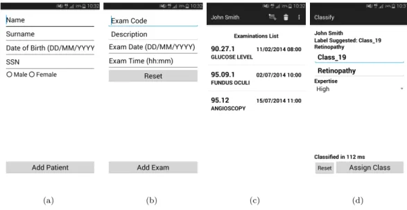
This section describes the main functionalities of the proposed mobile applications, while some example screenshots are reported in Figure 2.4.

New patients canregister to the application by inserting reference information as their fiscal code and birthdate (Figure 2.4(a)). The application allows both visualizing and updating the list of examinations underwent by the patient (Figures 2.4(b)and 2.4(c)). Any new underwent examination can be inserted by specifying the examination name

(30)

and code together with the date and time the patient underwent the examination. To enhance usability, the autocomplete feature is used for entering the examination name and code. Moreover, only one of the two fields must be specified, while the other is automatically filled by the application. For the diabetes dataset considered in this study, examination codes have been defined based on the ICD 9-CM (International Classification of Diseases, 9th revision, Clinical Modification) [25].

Through the application, the patient can be classified into one of a set of predefined categories based on his/her examination history and a precomputed classification model (Figure 2.4(d)). Moreover, the application allows collecting feedbacks and suggestions

from the domain expert on the proposed categorization. Specifically, he/she can either confirm this categorization or suggest an alternative one, by also specifying his/her degree of expertise in the provided feedbacks (Figure 2.4(d)).

In the medical domain, possible end-users of the application are mainly medical staff and patients to some extent. The application can support the medical staff in the patient evaluation by automatically proposing the patient classification into one out of a set of predefined categories. This automatic categorization can be a valuable support since usually the classification model is computed considering large data collections, and tuned to guarantee an accurate classification. Medical staff still preserves the possibility of proposing an alternative classification based on his/her degree of expertise. The application can also support patients in a self-evaluation of their condition.

The proposed architecture includes mobile devices (e.g., tablet, smartphone) running the application and a server storing the collection of patient examination histories used for creating the classification model. A web server provides functionalities to query this repository and read/insert new data from the application.

To minimize data exchange between the server and the mobile devices at any new classi-fication request, once generated on the server the classiclassi-fication model is downloaded on the mobile devices running the application. Consequently, any new classification request is locally processed by accessing the copy of the classification model stored on the mobile device. On the other hand, this local copy can be periodically updated by downloading the new version of the model generated on the server. More in detail, the classification model based on decision trees is stored on a text file as a list of if-then-else rules.

To allow enriching the central data repository available on the server, new data collected on the mobile device can be transmitted to the central server using the application. New data includes newly registered patients, updated examination histories and feedbacks provided by the domain expert. This enriched data collection can be later used for recomputing the classification model, aimed at increasing the classification accuracy.

(31)

(a) (b) (c) (d)

Figure 2.4: Mobile app: (a) patient registration, (b) insertion of a new examination done by the patient, (c) visualize patient examination history, (d) patient classification

2.1.7 Experimental results

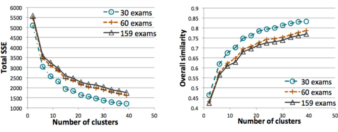
This section presents the results of the experiments with theMLDAframework regard-ing (i)quality evaluation for the computed cluster sets, (ii)execution timefor cluster set computation, and (iii) impact of data dimensionality, given by the number of different examinations used to describe patient histories, on the quality of the cluster sets. The

MLDAmethodology has been validated on a real collection of examination log data for

diabetic patients.

2.1.7.1 Dataset

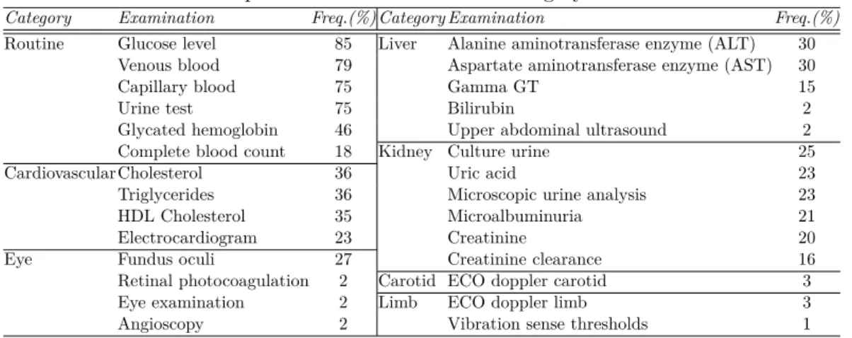
As a main reference case study we considered a real dataset of (anonymized) diabetic patients collected by an Italian Hospital. The diabetic patients dataset contains the examination log data of a set of 6,380 patients with overt diabetes, covering the time period of one year. Both male and female patients in a wide age range are included. The domain of the examinations includes 159 different examination types. Table2.5lists the most frequent examinations including routine examinations as well as more specific di-agnostic tests for diabetes complications with varying degrees of severity. Complications due to diabetes can affect for example the cardiovascular system, eyes, and liver. The diagnostic and therapeutic procedures are defined using the ICD 9-CM (International Classification of Diseases, 9th revision, Clinical Modification) [25].

(32)

Table 2.5: Most frequent examinations for each category in the diabetes dataset

Category Examination Freq.(%) Category Examination Freq.(%)

Routine Glucose level 85 Liver Alanine aminotransferase enzyme (ALT) 30 Venous blood 79 Aspartate aminotransferase enzyme (AST) 30

Capillary blood 75 Gamma GT 15

Urine test 75 Bilirubin 2

Glycated hemoglobin 46 Upper abdominal ultrasound 2 Complete blood count 18 Kidney Culture urine 25

Cardiovascular Cholesterol 36 Uric acid 23

Triglycerides 36 Microscopic urine analysis 23 HDL Cholesterol 35 Microalbuminuria 21

Electrocardiogram 23 Creatinine 20

Eye Fundus oculi 27 Creatinine clearance 16

Retinal photocoagulation 2 Carotid ECO doppler carotid 3 Eye examination 2 Limb ECO doppler limb 3 Angioscopy 2 Vibration sense thresholds 1

2.1.7.2 Evaluation setup and parameter configuration

The MLDA framework has been implemented as follows. To perform the multiple-level cluster analysis, the DBSCAN, K-means and K-medoids algorithms available in the RapidMiner toolkit have been used, and they have been applied in a multiple-level fashion. RapidMiner is an open-source platform including a number of data mining algorithms [26]. For a more accurate evaluation of the multiple-level strategy, also the standard (not multiple-level) K-means, K-medoids, and DBSCAN algorithms have been considered for performance comparison.

We developed in Java programming language the procedures for transforming the patient examination log data into the corresponding VSM representation using the TF-IDF weighting score, and for cluster evaluation through the SSE, silhouette, and overall similarity measures. Procedures for cluster evaluation have been implemented as a RapidMiner plugin. The procedure for Rand Index computation has been developed in Python programming language.

For K-means and K-medoids methods, experiments have been run by varying the K parameter, corresponding to the number of clusters in the final cluster set. For bisecting algorithms, this set is computed with K-1 iteration levels of the bisecting approach. For refined algorithms, the refinement process has been run for each final cluster set provided by bisecting algorithms. The usual approach has been adopted to address the problem of centroids and medoids initialization for bisecting algorithms, and for standard K-means and K-medoids when considered for performance comparison. Multiple runs, each with set of randomly chosen initial centroids (resp. medoids) have been performed, and then the cluster set with the minimum SSE has been selected. Specifically, RapidMiner pa-rameters maximum number of random initialisations and maximum number of iterations for each initialisation have been set to 50 and 300, respectively, for K-means methods.

(33)

The same parameters have been set to 10 and 100 (default values in RapidMiner) for K-medoids methods because of their relevant execution time on the considered use case (see Section2.1.7.4).

For the multiple-level DBSCAN, in setting the number of iterations, and the Eps and M inP ts values at each iteration level, we aimed at avoiding clusters with few patients, to discover representative examination sets, and at limiting the number of outlier pa-tients, to take into account the contribution of various examination histories. Clusters should show good cohesion and separation (i.e., silhouette values greater than 0.5). Dif-ferent Eps and M inP ts values have been selected at each iteration level due to the different data distribution of the dataset portion locally analyzed. This portion tends to be progressively sparser because it includes subsets of patients with more and more specific examinations (see Section 2.1.8). Consequently, at each subsequent iteration level, smaller M inP ts values are progressively selected to define a dense area region. The Eps value has been then locally tuned by trading-off the quality of the cluster set and the number of outlier patients.

Maximal sequential patterns have been extracted using the VMSP algorithm [27] avail-able at [28]. This algorithm has been adopted because it uses a data vertical representa-tion for a depth-first explorarepresenta-tion of the search space, that has been shown to be effective in various domains.

To create the classification model, the decision trees algorithm available in the Rapid-Miner toolkit have been used. The mobile application has been developed on the Android environment version 4.4.

Experiments were performed on a 2.66-GHz Intel(R) Core(TM)2 Quad PC with 8 GBytes of main memory, running linux (kernel 3.2.0).

2.1.7.3 Cluster quality evaluation

The quality for the computed cluster sets has been evaluated based on the SSE (for K-means and K-medoids methods), Silhouette (for DBSCAN methods), and overall similarity (for all methods) measures.

Evaluation of K-means methods

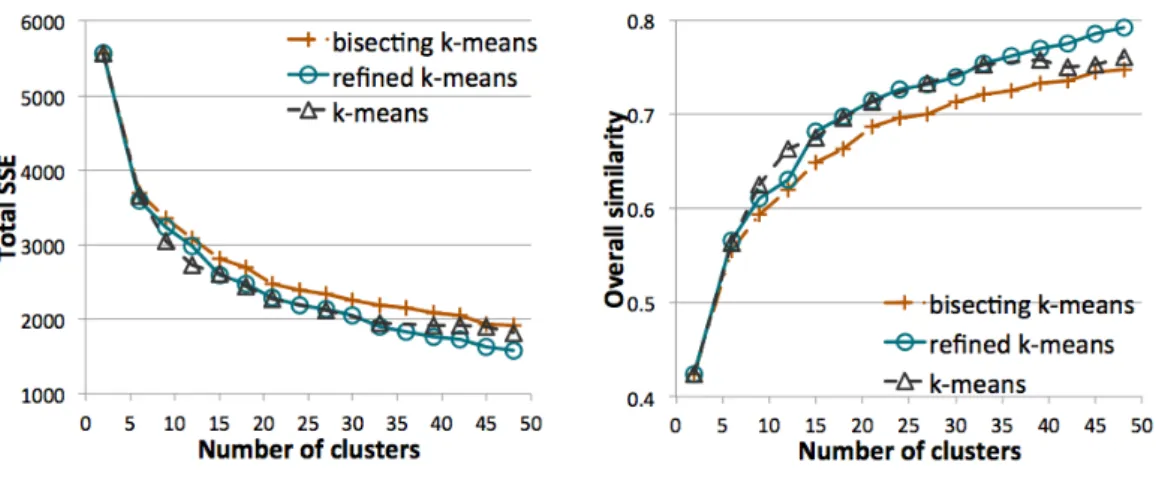
For all K-means methods, the total SSE measure progressively decreases, and the overall similarity measure progressively increases, when growing the value of K and thus the number of clusters (see Figure2.5). The bisecting K-means algorithm always provides the worst results for both measures, i.e., the cluster sets with the highest total SSE and

(34)

Figure 2.5: K-means methods: quality of the cluster set when varying the number of clusters

the lowest overall similarity values. Nevertheless, the refined K-means algorithm always provides better results than bisecting K-means, showing that the use in a subsequent clustering phase of the “centroids" computed with the bisecting K-means algorithm can improve the quality of the final cluster set.

Compared to standard K-means, the refined K-means algorithm provides better results when increasing K (about K>30, i.e., more than 30 clusters). It is worse than standard K-means when a lower value of K is considered (5≤K≤15, i.e., between 5 and 15 clusters). It follows that the final cluster set can benefit from a multiple-level clustering strategy when the number of iteration levels, and thus the final number of clusters, increases. The K parameter can be selected based on the desired number of clusters and the expected quality of the cluster set.

As a reference example, Table 2.6 reports the main characteristics of the solution with 32 clusters, in terms of number of patients, different examinations, SSE and overall similarity for each cluster.

Evaluation of K-medoids methods

The experimental results reported in Figure2.6show that K-medoids methods exhibit a similar behavior to K-means ones. The bisecting K-medoids algorithm always provides the worst results in terms of overall similarity and total SSE values. The refined K-medoids algorithm always improves bisecting K-K-medoids and provides comparable results to standard K-medoids.

K-medoids methods showed a very high computational cost which limited their appli-cability in the _MLDA framework (see Section 2.1.7.4). Due to this cost, solution sets with a larger number of clusters have not been generated.

(35)

Table 2.6: Detailed clustering results for refined K-means C1 C2 C3 C4 C5 C6 C7 C8 C9 C10 C11 C12 Number of patients 96 172 169 97 124 239 233 206 13 88 38 376 Number of examinations 42 39 25 18 52 51 44 40 31 34 38 60 SSE 67.6 112 39.9 8.72 43.3 105 88.7 65.5 5.17 22.4 14.7 134 Overall similarity 0.51 0.50 0.80 0.92 0.70 0.63 0.67 0.72 0.70 0.79 0.67 0.69 C13 C14 C15 C16 C17 C18 C19 C20 C21 C22 C23 C24 Number of patients 18 78 402 231 351 50 47 26 201 182 226 146 Number of examinations 33 30 56 44 67 28 34 51 37 41 46 54 SSE 7.43 38.3 137 100 149 24.2 17.6 15.7 98.7 48.9 76.3 113 Overall similarity 0.66 0.61 0.70 0.63 0.64 0.60 0.69 0.54 0.59 0.77 0.71 0.45 C25 C26 C27 C28 C29 C30 C31 C32 Number of patients 74 1,126 509 61 169 170 257 205 Number of examinations 39 35 35 40 20 24 28 30 SSE 58.7 55.3 57 34.2 22.5 65.5 43.9 55.8 Overall similarity 0.43 0.96 0.90 0.57 0.88 0.76 0.85 0.76 Whole cluster set

Total SSE 1,926.01

Overall similarity 0.75

Figure 2.6: K-medoids methods: quality of the cluster set when varying the number of clusters

Evaluation of DBSCAN methods

As reported in Table 2.7, when iterating the multiple-level DBSCAN approach for four levels, 32 clusters are computed in total showing good overall similarity and silhouette values (greater than 0.5). These clusters globally includes 3,510 patients (about 55% of the diabetes dataset). Most patients belong to clusters computed at the first level, while a comparable number of patients is included in clusters computed at the next levels. After four iterations, 2,870 patients are labeled as outliers and remain unclustered. Note that these patients can be additionally clustered by iterating the approach for more levels.

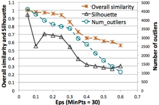
Clustering about 55% of the patients using the standard DBSCAN algorithm generates a lower quality cluster set than when using the multiple-level DBSCAN approach. To deepen into the analysis of this point, Figure2.7plots the silhouette and overall similarity

(36)

Figure 2.7: DBSCAN algorithm: quality of the cluster set and number of outlier patients when varying theEps value (M inP ts=30)

values, and number of outlier patients, when the whole patient collection is analyzed using the standard DBSCAN. With parameters Eps=0.36 and M inP ts=30, a cluster set is generated including almost the same number of patients than the cluster set from the multiple-level DBSCAN approach, but with a significantly lower quality. The overall similarity value is 0.73 and the silhouette is 0.4 (i.e., lower than 0.5), while these values are 0.85 and 0.55, respectively, for the multiple-level DBSCAN when iterated for four levels (see Table 2.7). It follows that, also for the DBSCAN method, the final cluster set can benefit of the multiple-level strategy.

Clusters computed with four level iterations are described in Table2.8in terms of their number of patients, different examinations and overall similarity value, while silhouette plot is reported in Figure2.8. Clusters mainly show a rather prominent silhouette. Few patients have negative silhouette values in clusters computed at the first level, i.e., 198 patients out of 1,764 in cluster C₁₁, 2 patients out of 223 in C₂₁ and 7 patients out of 294 in C₄₁. At the fourth level, cluster C₃₄ shows a less prominent silhouette, but the average silhouette value is almost 0.5.

Table 2.7: Clustering results for multiple-level DBSCAN 1st level 2nd level 3rd level 4th level (MinPts, Eps) (30, 0.3) (30, 0.5) (20, 0.5) (10, 0.35)

Number of clusters 11 5 4 12

Number of patients 2,872 260 104 274

Silhouette 0.54 0.61 0.66 0.6

Overall similarity 0.85 0.86 0.89 0.94

Whole cluster set

Number of clusters 32

Number of clustered patients 3,510 Number of outliers 2,870

Silhouette 0.55