Semi-supervised multi-layered clustering model for intrusion detection

journal homepage: www.elsevier.com

Semi-supervised Multi-Layered Clustering

Model for Intrusion Detection

Omar Y. Al-Jarrah

, Yousof Al-Hammdi

, Paul D. Yoo

, Sami Muhaidat

,

Mahmoud Al-Qutayri

a_{Department of Electrical and Computer Engineering, Khalifa University of Science, Technology and Research (KUSTAR)}

, Abu Dhabi, UAE

b_{Centre for Electronic Warfare, Information and Cyber (CEWIC), Cranfield University, Defence Academy of the United Kingdom}

, Shrivenham, Swindon, SN6 8LA, United Kingdom

Abstract

A Machine Learning (ML) -based Intrusion Detection and Prevention System (IDPS) requires a large amount of labeled up-to-date training data, to effectively detect intrusions and generalize well to novel attacks. However, labeling of data is costly and becomes infeasible when dealing with big data, such as those generated by IoT (Internet of Things) -based applications. To this effect, building a ML model that learns from non- or partially-labeled data is of critical importance. This paper proposes a novel Semi-supervised Multi-Layered Clustering Model (SMLC) for network intrusion detection and prevention tasks. The SMLC has the capability to learn from partially labeled data while achieving a comparable detection performance to supervised ML-based IDPS. The performance of the SMLC is compared with well-known supervised ensemble ML models, namely, RandomForest, Bagging, and AdaboostM1 and a semi-supervised model (i.e., tri-training) on a benchmark network intrusion dataset, the Kyoto 2006+. Experimental results show that the SMLC outperforms all other models and can achieve better detection accuracy using only 20% labeled instances of the training data.

c

2015 Published by Elsevier Ltd.

KEYWORDS:

Semi-supervised intrusion detection, machine learning, classification, ensembles, and big data.

1. Introduction

As we head towards the IoT (Internet of Things) era, the number of objects that have the capability to col-lect and exchange data is increasing at a phenomenal rate. This is due to the advances in semiconductors, networking, communications, sensors, and Internet re-lated technologies, which result in ubiquitous connec-tivity to vast arrays of Internet-based infrastructures, services and applications, such as banking and energy utility. Many applications in different fields, such as social networking, economy, healthcare, industry and

∗

Omar Y. Al-Jarrah (Corresponding au-thor)(email:[email protected]).

1_{Yousof Al-Hammadi, Sami Muhaidat, Mahmoud}

Al-Qutayri (email:{yousof.alhammadi, sami.muhaidat, mqutayri}@kustar.ac.ae).

2_{Paul D. Yoo (email:[email protected]).}

science, produce a huge amount of data namely big data. In fact, it is predicted that there will be as much data created as was created in the entire history of planet Earth, with 90% of current data were created in the last couple of years [1]. The emergence of big data combined with the disappearing network boundaries and the sophisticated attacks elevate the risk of net-work intrusions. Maintaining the integrity and secu-rity of the Internet-based services and infrastructures, particularly from cyber-attacks, is of paramount im-portance. Smart cities that are evolving based on IoT technologies, for example, will simply not function re-liably without agile secure infrastructures.

An Intrusion Detection and Prevention System (IDPS) is an essential component of networks’ secu-rity infrastructure, as it monitors, detects, and iden-tifies potential intrusions. IDPSs are classified based

on their ability to recognize known and unknown at-tacks [2]. Rule-based IDPSs make their decisions based on rule-sets defined by domain experts. Such IDPSs are successful in detecting known attacks, but they have limited capabilities in front of novel at-tacks. Given the significant increase in network traffic, finding and coding rule-sets of rule-based IDPSs be-come difficult and time-consuming [3]. An anomaly-based IDPS builds a model of normality and consid-ers deviation from this model as an attack. Although anomaly-based IDPSs are shown to be capable of de-tecting novel/unknown attacks, they require pure train-ing datasets of normal traffic in order to build their detection models. However, collecting pure training datasets of benign/normal network traffic is difficult due to the high similarity between the normal and the malicious traffic.

Machine learning (ML) algorithms have been adopted for IDPSs due to their model-free proper-ties, which allow them to learn complex malicious and normality models [2]. Although ML algorithms brought significant advantages to IDPSs by automat-ing the generation process of the models/rules of de-tection, they have been deployed in limited scale in real-world [2, 4]. This is due to the fact that super-vised ML-based IDPSs require a sufficient supply of labeled training data. Unfortunately, data labeling, which is normally done by domain expert, is expen-sive in terms of time and cost [3]. In contrast, un-supervised ML-based IDPSs, such as clustering-based IDPS, build models with unlabeled data. However, the performance of unsupervised ML-based systems, in general, is not as good as the performance of su-pervised ML-based systems [5]. Thus, with the ever-increasing size of data, there is a need for powerful unsupervised or semi-supervised learning algorithms that can perform the tasks of IDPS.

This paper introduces a novel Semi-supervised Multi-Layered Clustering (SMLC) model for network intrusion detection and prevention tasks. The pro-posed model mitigates the deployment issues of the existing supervised ML-based IDPSs as it can achieve comparable/better performance with partially labeled data. The SMLC builds an ensemble model of multi-ple randomized layers using K-Means algorithm. The local learning models of the SMLC are learned from the resultant clusters at different layers. The final pre-diction of a test instance is obtained by choosing the classification with the most votes of all decisions from all layers. The contributions of this work are as follow:

• Design and development of a semi-supervised model for network intrusion detection tasks. The proposed model utilizes the fact that instances of the same class-type stay close in the Euclidean space to reduce data labeling error, which im-proves the final detection accuracy (Section 3).

• Relying on the concept of weighted Euclidean

distance measure and atomic clusters, we argue that the time to update model and classification time of the proposed model can be significantly reduced by building binary classifiers at non-atomic clusters only (Section 3.1).

• Comparisons of the SMLC with the well-known supervised ensemble ML models, namely, Ran-domForest (RF), Bagging, and AdaBoostM1, and a semi-supervised, the tri-training algorithm, in terms of model accuracy, detection rate, false alarm, F-score, and Matthews correlation coef-ficient on a benchmark network intrusion dataset, the Kyoto 2006+. (Section 4).

This paper is organized as follows. Section 2 provides an overview of current development of ML models for IDPS. Section 3 describes the proposed SMLC model. Section 4 discusses the settings of the experiments and the results. Section 5 presents the conclusions of this work.

2. Related Work

Machine Learning (ML) refers to computer algo-rithms that learn from experiences without being pro-grammed. A ML algorithm takes data of instance space as an input and outputs a hypothesis of a defined hypothesis space that describes regularities in the data [2]. Supervised ML algorithms build learning mod-els on training dataset of paired input instances and their corresponding labels or outputs. On the other hand, unsupervised algorithms group input instances into clusters based on some similarity measures. Its worth noting that the ability of a ML algorithm to learn the underneath patterns in a training data and general-ize to unseen events depends on the quality and quan-tity of the training data [6]. Recently, combining ML techniques, which are also known as ensemble mod-els, has gained significant attention in ML community as they often perform better than individual models and adapt quickly to new concepts [7, 8, 9]. Basically, an ensemble model generates multiple base classifiers that commit error on identical data pattern indepen-dently. The final verdict of ensemble model is derived from the individual predictions of the constituent base classifiers. Clustered ensemble [10], Bagging [11] and Boosting [12] are well-known ensemble mod-els. Unlike previously mentioned ML models, semi-supervised models use both labeled and unlabeled data to build their final hypothesis [13, 14]. Several studies in literature, such as, [15, 16, 17, 18, 19], have adopted semi-supervised learning approaches for intrusion de-tection and prevention tasks. Wagh and Kolhe [15] presented a semi-supervised approach to intrusion de-tection. The proposed approach uses the most con-fident filtered data from testing dataset to refine the existing training dataset, which is used automatically to train the system again. Chenet al. [16] proposed

two semi-supervised classification methods, Spectral Graph Transducer and Gaussian Fields Approach, to detect unknown attacks and one semi-supervised clus-tering method, the MPCK-means. Liet al. [17] pro-posed an intrusion detection algorithm based on the semi-supervised fuzzy clustering where a few labeled instances are used as seeds to initialize the classifier of the system. Chiu et al. [18] introduced a semi-supervised learning mechanism to build an alert filter that reduces false alarms and keeps high detection rate. The proposed mechanism uses Two-Teachers-One-Student (2T1S) as a learner for the proposed ML en-gine. Yuxin Menget al. [19] applied a disagreement-based semi-supervised learning algorithm to construct a false alarm filter and investigated its performance on alarm reduction in a network environment.

Contrary to the co-training-based IDPS introduced in [20], the proposed SMLC does not require generat-ing different views of the data. More importantly, the SMLC presents a new methodology to generate semi-supervised ensemble model. In addition, the SMLC does not put any constrains on the used supervised algorithm. The SMLC model augments the learning process of its local learning models by: 1) utilizing the unlabeled data and 2) dividing the training data into mutually exclusive clusters at each layer, exploiting that instances of the same class-type tend to stay close to each other in the Euclidean space. The SMLC en-hances its overall detection accuracy by: 1) providing diversity among its base classifiers as it generates mul-tiple randomized layers using the K-Means clustering, 2) identifying difficult- and easy-to-classify instances, and 3) employing majority vote to find the final pre-diction of an instance.

3. Proposed Semi-supervised Multi-Layered Clus-tering Model

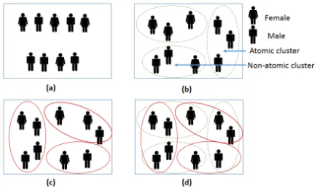
In this section, we present our Semi-supervised Multi-Layered Clustering (SMLC) model based on the concept of data clustering. The SMLC adopts the work presented in [21] and exploits that resultant clus-ters of the K-Means algorithm depend on the initial-ization parameters (e.g., seed, number of clusters), to provide diversity among its base classifiers [21]. Data instances might be assigned to different clusters when different initialization parameters are used [22]. In this context, a layer is defined as an object of K-Means us-ing a randomized parameter (i.e., seed). Thus, a dat-apoint/instance might belong to different clusters on different layers. Clusters at different layers might have overlapping but non-identical data, though; clusters at the same layer are mutually exclusive and might have datapoints of one or multiple classes. To clarify this, consider a dataset of two classes as in Fig. 1. (a). In this context, as in Fig. 1. (b), a layer is defined as an object of a K-Means clustering algorithm based on one set of initialization parameters (i.e., seed). Thus,

a datapoint/instance might belong to different clus-ters on different layers as in Fig. 1. (b), and (c). Clusters at the same layer are mutually exclusive (i.e., non-overlapping). However, clusters at different lay-ers might have overlapping but no-identical data as in Fig. 1. (d). Hence, clusters at different layers might be used to build diverse base classifiers, which can be used to construct an ensemble model that covers the whole decision space as in Fig. 1. (d).

Fig. 1: (a) a dataset of two classes (male and female). (b) resultant clusters of K-Means algorithm using seed 1 (i.e, layer 1). (c) resul-tant clusters of K-Means algorithm using seed 2 (i.e., layer 2). (d) a projection of the resultant clusters at different layers.

The SMLC generates multiple layers of randomized K-Means algorithm. Training dataset is fed to all lay-ers in the SMLC model and portioned intoKclusters at each layer. The resultant clusters at each layer might have datapoints/instances of different classes or one class. We refer to the cluster of instances of one class type as an atomic cluster (e.g., cluster 3 in Fig.1. (b)), whereas, non-atomic cluster is defined as the cluster of instances of multiple classes (e.g., cluster 2 in Fig. 1. (b). In order to infer dependencies of the data, the SMLC builds local learning models on the resultant clusters at each layer. Basically, it builds binary clas-sifiers at non-atomic clusters and remembers the class label of atomic clusters. In the following subsections, we describe 1) the data clustering using K-Means and propose weighted Euclidean distance, 2) the training, 3) and testing processes of the SMLC model.

3.1. Data Clustering and Weighted Euclidean Dis-tance

The K-Means clustering algorithm is well-known and widely used due to its simplicity and ease of im-plementation [23]. However, the resultant clusters of K-Means depend, heavily, on the initialization param-eters. The SMLC exploits this property to provide di-versity among its base classifiers. It also builds local learning model on the generated overlapping but not identical clusters at different layers.

Let x1,x2, ...,xn be a set of instances in

d-dimensional space and K is a predefined number of clusters. The K-Means algorithm minimizes the

ob-jective function given by [22]: F(x1,x2, ...,xN)= K X k₌1 X xi∈ck kxi−x¯kk2, (1)

whereckdenotes thekthcluster,

¯ xk= 1 nk X xi∈ck xi, (2)

is the center of the kth cluster, and nk is the number

of instances in kth cluster. k.kdenotes the Euclidean norm used by the K-Means algorithm. The algorithm starts withKinstances that represent the centroids of the clusters. Each instance in the training dataset is assigned to the centroid of the closest cluster and the mean of the instances in the same cluster is calcu-lated. The procedure is repeated iteratively until con-vergence or an exit condition is satisfied.

Distance measure is an important aspect to con-sider in the application of the K-Means algorithm. Eu-clidean distance is the most widely used distance mea-sure, and is given by the following [22]:

d(x,z)= v u t d X j=1 (xj−zj)2, (3)

wheredis the number of dimensions or features. xj

andzj are the values of the jth attribute of x and z,

respectively. Although the Euclidean distance works well for clusters with spherical homogeneous covari-ance matrices, it still treats all attributes equally when computing the distance between instances. Such ap-proach is not desirable when some attributes are more important to discriminate between patterns [24]. As such, deploying such measures might yield low perfor-mance and affect the required number of iterations un-til the convergence of the K-Means algorithm. There-fore, we introduce the use of a weighted Euclidean dis-tance measure based on the observation that different attributes might have a strong impact on the resultant partitions of data. The weighted Euclidean distance assigns a weight for each attribute based on its signif-icance in distinguishing between class types. These weighted attributes can lead to a higher probability of obtaining atomic clusters with lower value ofK (i.e., number of clusters), which have the following advan-tages:

1. Reducing the overall complexity of the proposed model. This is mainly due to the fact that the SMLC uses the class labels of atomic clusters only, eliminating the need for building binary classifiers.

2. Increasing the prediction efficiency of the sys-tem, since the overall number of binary classifiers used is reduced. In this case, the test instances are examined by fewer binary classifiers, which reduces the testing time per instance.

In this paper, the Information Gain Ratio (IGR) [25] is used as an attribute’s weight, since it reflects the utility and significance of the attribute in detecting a class type, which is given by:

IGR(Y,Aj)=

H(Y)−H(Y|Aj)

H(Aj)

, (4)

whereY is the class, andAjis the jthattribute. Here,

H(.) is the entropy function given by: H(X)=−X

∀i

P(xi) log2[P(xi)], (5)

where,P(.) is the probability operator, andiis an index of the probabilities in a given input. Hereafter, the pro-posed weighted Euclidean distance based on theIGR is given by: d(x,z)= v u t d X j=1 wj(xj−zj)2, (6)

wherewjdenotes the weight of the jthattribute. The

weights of the attributes are calculated and then passed to each layer in the SMLC. The value ofIGRof thejth attribute is assigned towjas follows:

wj=IGR(Y,Aj), (7)

3.2. Training Process of The SMLC

The SMLC deals with partially labeled data. In this case, the training data includes labeled and un-labeled instances. Each labeled instance is given a class label. On the other hand, unlabeled in-stances are not given any label. Let the train-ing dataset be denoted by T = {TLabeled,TUnlabeled},

where TLabeled = {(x1,y1),(x2,y2), ...,(xn,yn)}, n

de-notes the number of labeled instances in TLabeled,

TUnlabeled = {(xn+1),(xn+2), ...,(xN)}, N is the

num-ber of instances inT,xi denotes theithinstance (i.e.,

xi=<xi1,xi2, ...,xid >),drepresents the number of

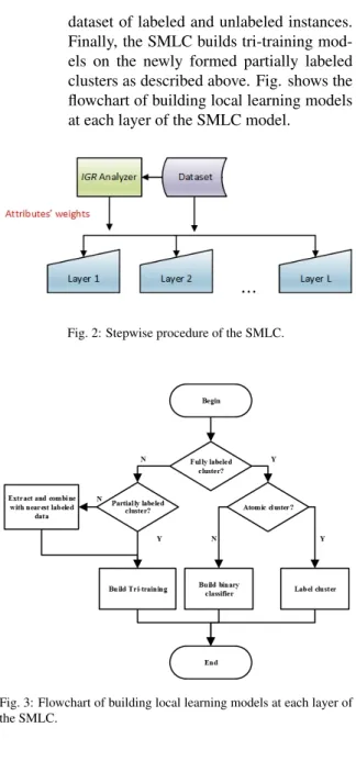
at-tributes, andyi∈Yis the class label set. Fig. 2 shows

the stepwise procedure of the SMLC. The training pro-cess of the SMLC has two main phases:

1. The SMLC generates overlapping but diverse clusters at different layers by using different ini-tialization parameters set (i.e., random seed). The K-Means generates diverse clusters at different layers, {C1,2, ...,C1,K}, ...,{CL,2, ...,CL,K}. Here we modified the K-Means algorithm to use the distance measure illustrated in (6). wj is

calcu-lated according to (7) and its value is obtained from the IGRAnalyzer. It should be noted that IGRAnalyzer uses theTLabeledonly to calculate

the weights of the attributes. The class labels of the training instances have not been considered in data clustering because the training dataset con-tains labeled and unlabeled instances.

2. The resultant cluster could be one of three types: a) fully labeled cluster that contains labeled in-stances only; b) partially labeled cluster that con-tains labeled and unlabeled instances; and c) un-labeled cluster. During the second phase, the SMLC identifies fully labeled, partially labeled, unlabeled clusters and builds a learning model on each cluster as follows:

• In the case of fully labeled clusters, the SMLC identifies atomic and non-atomic clusters at each layer. Equation (8) illus-trates how a class distribution function is calculated for each clusterCl,k:

FCl,k(yj)= X ∀(xi,yi)∈Cl,k θ(yj,yi), (8) where, θ(yj,yi)= ( 1 ifyj=yi 0 otherwise (9)

The clusterCl,kis defined as atomic if it sat-isfies the following:

Max∀yj∈Cl,k(FCl,k(yj))

P

∀yj∈Cl,kFCl,k(yj)

=1. (10)

Thereafter, the SMLC builds binary classi-fiers with non-atomic clusters and remem-bers the class label of atomic clusters. • The SMLC builds tri-training models with

partially labeled clusters, which contain labeled and unlabeled instances, at each layers. A tri-training model builds three non-identical classifiers with the labeled instances in each partially labeled cluster [26]. The three classifiers are then refined using unlabeled instances in the partially la-beled cluster. In each iteration of the tri-training, an unlabeled instance is labeled for a classifier if the other two classifiers agree on the labeling [26]. Unless the three base classifiers are drawn from different distribu-tions, they will always agree on the class la-bel of the unlala-beled instance. Therefore, the base classifiers are initially trained on boot-strapped training datasets from the labeled instances. The final hypothesis is produced via majority voting among all individual de-cisions of the three base classifiers. • The resultant clusters might contain

unla-beled instances only. In that case, at each layer, the SMLC finds the nearest neigh-bor labeled instances from the labeled por-tion of the training dataset (TLabeled) to the

centroids of the unlabeled clusters. Then, it combines the unlabeled clusters with its corresponding labeled data to form a new

dataset of labeled and unlabeled instances. Finally, the SMLC builds tri-training mod-els on the newly formed partially labeled clusters as described above. Fig. shows the flowchart of building local learning models at each layer of the SMLC model.

Fig. 2: Stepwise procedure of the SMLC.

Fig. 3: Flowchart of building local learning models at each layer of the SMLC.

3.3. Testing Process of The SMLC

The testing process of a test instance begins with finding the nearest clusters centroid at each layer of the SMLC. The cluster that has the minimum distance between its centroid and the testing instance at each layer is selected as the appropriate cluster. Then, the correspondent classifier at that layer is used to predict the class type of the testing instance. The final label of the testing instance is determined by the majority vote corresponding classifiers at different layers.

4. Evaluation and Analysis

Thorough evaluation of an IDPS is of crucial in-terest as many approaches fail to meet what are ex-pected from them in real-world scenario [4]. This re-quires an appropriate dataset that represents the real-world scenario. The most widely used datasets are DARPA/Lincoln packet traces [27], [28] and KDD Cup [29] derived from it, however, these datasets

# Name Description

1. Duration The length (seconds) of the connection. 2. Service The connection’s service type,e.g., http, telnet. 3. Source bytes The number of data bytes sent by the source IP address. 4. Destination

bytes

The number of data bytes sent by the destination IP address.

5. Count The number of connections whose source IP address and desti-nation IP address are the same to those of the current connection in the past two seconds.

6. Same srv rate % of connections to the same service in Count feature. 7. Serror rate % of connections that have SYN errors in Count feature. 8. Srv serror rate % of connections that have SYN errors in Srv count (the number

of connections whose service type is the same to that of the current connection in the past two seconds) feature. 9. Dst host count Among the past 100 connections whose destination IP address

is the same to that of the current connection, the number of connections whose source IP address is also the same to that of the current connection.

10.Dst host srv count

Among the past 100 connections whose destination IP address is the same to that of the current connection, the number of connections whose service type is also the same to that of the current connection.

11.Dst host same src port rate

% of connections whose source port is the same to that of the current connection in Dst host count feature.

12.Dst host serror rate

%of connections that have SYN errors in Dst host count feature.

13.Dst host srv serror rate

% of connections that SYN errors in Dst host srv count feature.

14.Flag The state of the connection at the time the connection was writ-ten.

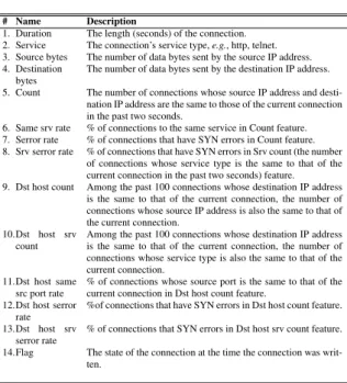
Table 1: Features of the Kyoto 2006+dataset.

are now outdated. In this paper, we use the Ky-oto 2006+ dataset [30] to evaluate the performance of the proposed model as well as other ML models. The Kyoto 2006+dataset contains real network traf-fic data collected from Nov 2006 to Aug 2009. It has 93,076,270 sessions where 50,033,015 are normal sessions, 42,617,536 are known attacks sessions, and 425,719 are unknown attacks sessions.

Known attacks refer to networks sessions that trig-gered IDS alarm. On the other hand, unknown at-tacks refer to networks sessions that did not trigger IDS alarm but contain shellcodes. Each session has 24 attributes, of which 14 attributes are derived from the attributes of the KDD99 dataset and represent the most significance and essential characteristics of a network session. The attributes of contents are excluded, be-cause they are not suitable for Network Intrusion De-tection System (NIDS) and need domain knowledge to extract them. Additional 10 attributes, which can be used for further analysis and evaluation of NIDS and determining the kind of attacks happened in the network, were extracted and added to the attributes of the dataset. As our main objective is to detect attacks regardless of their type (known or unknown attack), we consider the fourteen essential attributes and we further give the known and unknown attacks the same label. Table 1 shows descriptions of the attributes of the Kyoto 2006+dataset, excluding the class label.

4.1. Data Selection and Preprocessing

Based on the findings in [31], data of five days of traffic is an appropriate learning size when the Kyoto 2006+dataset is used. Therefore, we use the data from 1st to 5th January as training dataset, which has 560, 527 instances.

Labeled % Normal Attacks Unlabeled JSD

1 3,216 2,390 554,921 1.304×10−3 5 16,077 11,950 532,500 3.392×10−4 10 32,150 23,903 504,474 1.904×10−4 20 63,990 48,116 448,421 9.692×10−5 30 96,179 71,980 392,368 6.203×10−5 40 128,290 95,921 336,316 4.070×10−5 50 160,529 119,735 280,263 2.789×10−5 60 192,542 143,775 224,210 1.844×10−5 70 224,480 167,889 168,158 1.209×10−5 80 256,676 191,746 112,105 7.024×10−6 90 288,530 215,945 56,052 3.258×10−6

Table 2: Statistics of the selected training datasets and Jensen-Shanon divergence.

Dataset Normal Attacks Total Training 320,764 239,763 560,527 Validation 484,408 272,561 756,969 Testing 323,301 181,345 504,646 Table 3: Statistics of the training, validation, and testing datasets.

We study the performance of the proposed SMLC model with the number of labeled instances in the training dataset. Initially, we randomly remove the la-bel of a specific percentage of instances in the train-ing dataset (e.g., 90%, 10%) and repeat the process 10 times. Then, we pick the best representative dataset of the ten partially labeled datasets. Here, we used the Jensen-Shannon divergence to select the best rep-resentative dataset based on the statistical similarity between the labeled portion of the dataset and the original fully labeled training dataset. The Jensen-Shannon divergence between two probability distribu-tions is given by [32]: JS D(P||Q)=1 2D(P||M)+ 1 2D(Q||M), (11) where M=1 2(P+Q), (12) D(P||Q)=X i

P(i) logP(i)

Q(i), (13)

and

0≤JS D(P||Q)≤1. (14) Table 2 shows the statistics of selected training datasets and the calculated Jensen-Shannon diver-gence measure (JSD).

We generate validation and test datasets by merging the data of 12 days of traffic, pulled from the last six months of the year 2008. The merged data includes the data of the 10th _{and 25}th_{of each month from July} to December in the year 2008. We replace the data of the 25thof September, 2008 by the data of the 23rd of September, 2008 since the dataset does not contain traffic of that day [31]. We use 60% of the merged data as a validation dataset and the remaining 40% as a test dataset. Table 3 shows the statistics of the training, validation and test datasets.

Actual Predicted Attack Predicted Normal

Attack TP FN

Normal FP TN

Table 4: Confusion matrix. 4.2. Performance Analysis

We compare the prediction capabilities of the SMLC model with the well-known supervised ensem-ble models, namely, RandomForest (RF) [33], Bag-ging [11], AdaBoostM1 [12] and the semi-supervised learning model, tri-training [26]. The results of the SMLC were obtained by modifying the Java code of Weka package [34]. The measures used to evaluate the performance of each classifier are as follows: clas-sification accuracy (Acc), detection rate (DR, a.k.a., sensitivity), false positive rate (FPR), F1-score (F1), and Matthews correlation coefficient (Mcc). These measures could be derived from the confusion matrix shown in Table 4.

True-Positive (TP) is the number of correctly clas-sified intrusions/attacks, True-Negative (TN) is the number of correctly classified normal connections, False-Negative (FN) is the number of incorrectly clas-sified intrusions as normal connections, and False-Positive (FP) is the number of incorrectly classified normal traffic as intrusions. Acc measures the clas-sifiers ability to correctly classify normal and attack traffics; DR is the number of intrusions detected by the model divided by the total number of attack in-stances in the test set; FPR refers to the percentage of normal traffic classified as intrusions; Mcc is a corre-lation coefficient between the observed and detected binary classification that has a value between -1 and +1, a coefficient of+1 represents a perfect detection, 0 means no better than random detection and -1 in-dicates total disagreement between detection and ob-servation. A high value of Mcc means more robust detection model. We aim for a high Acc, DR, F1 and Mcc, and low FPR. Acc= T P+T N T P+T N+FP+FN, (15) DR= T P T P+FN, (16) FAR= FP T N+FP, (17) F1= 2T P 2T P+FN+FP, (18) Mcc= √ (T P×T N−FP×FN) (T P+FP)(T P+FN)(T N+FP)(T N+FN). (19) 4.3. Parameters Tuning

The performance of the proposed model is con-strained by two parameters, number of layers (L), and

number of clusters (K). We have studied the perfor-mance of the SMLC model while varyingLandKand selected the values of LandKthat maximize the de-tection accuracy of the SMLC. Although the number of clusters is empirically selected, Davies-Bouldin In-dex (DBI) might be used to select the optimal number of clusters. DBI is a metric to evaluate clustering al-gorithm [35]. DBI considers the separation between different clusters and the scatter within each cluster. It is defined as the ratio of scatter of clusteriand the separation between cluster iand other clusters. The lower the value of DBI, the better the separation be-tween clusters and dense clusters.

The final decision of the proposed SMLC is derived from the individual decisions at different layers, aim-ing to eliminate the uncorrelated errors among base classifiers, which requires that each individual classi-fier commits its error independently from other base classifiers [36, 37]. Kohvai-Wolpert (KW) variance [38] has been used in the literature to compute the di-versity, which represents the correlation between base classifiers of an ensemble model [39]. Parameter tun-ing process might include findtun-ing the value ofKthat minimizes DBI and then find the value ofLthat max-imizes Kohvai-Wolpert (KW) variance.

For fair comparison, we optimized the selected su-pervised ensemble models by using Sequential Model-based Algorithm Configuration (SMAC) [40], which makes progressively better estimates by considering the configuration that outperforms the previous ones in every comparison made. We run the SMAC algo-rithm ten times for all selected models (i.e., RF, Bag-ging, and AdaBoostM1), where different seed is used in each iteration, then, we pick the best performing pa-rameters set among the resultant ten configurations of each model.

4.4. Comparative Performance Analysis

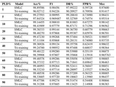
We compare the detection performance of the SMLC against the semi-supervised tri-training algo-rithm while varying the percentage of labeled data (PLD) in the training dataset from 1% to 90%. Table 5 shows the performance of both models. The detec-tion accuracy of both models is improved as the PLD increases. It is noticed that performance of tri-training reaches its maxima with a PLD of 40%. For exam-ple, the tri-training achieved a detection accuracy of 99.24700% when the PLD is 40%, whereas it correctly classifies 98.31208% of the testing instances with 90% PLD value. The SMLC shows almost a stable perfor-mance as its detection perforperfor-mance is positively cor-related with the PLD value. Moreover, the SMLC outperforms the tri-training algorithm in all perfor-mance measures. Of particular interest is the ability to achieve better detection accuracy using less PLD. For example, the Tri-training achieves a detection ac-curacy of 99.24700% using 40% PLD whereas the SMLC achieves a detection accuracy of 99.38333%

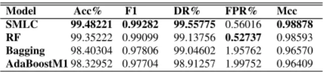
Model Acc% F1 DR% FPR% Mcc SMLC 99.48221 0.99282 99.55775 0.56016 0.98878 RF 99.35222 0.99099 99.13756 0.52737 0.98593 Bagging 98.40304 0.97806 99.04602 1.95762 0.96570 AdaBoostM198.32952 0.97704 98.91257 1.99752 0.96409

Table 6 shows the performances of different ensemble models on the testing dataset. The SMLC was given the following parameters: K=7 and L=3, RandomForest, Bag-ging and AdaBoostM1 were optimized by using SMAC algorithm and given the following parameters: weka.classifiers.trees.RandomForest I 161 K 0 S 1 depth 19 -num-slots 1, Bagging: weka.classifiers.meta.Bagging -P 164 -S 1 --num-slots 1 -I 9 -W weka.classifiers.trees.J48 decimal-places 0 – -S -C 0.089484066 -B -M 36 numdecimalplaces 0, AdaBoostM1: weka.classifiers.meta.AdaBoostM1 P 84 S 1 I 12 -W weka.classifiers.trees.J48 decimal-places 0 – -C 0.19157031 -B -M 1 -A -num-decimal-places 0.

Table 6: Performance of different models on Kyoto 2006+dataset when the training dataset is fully labeled.

using only 20% PLD. This is because the SMLC en-hances the detection performance of the base classi-fiers by building local learning models with the resul-tant data clusters, leading to reduction in the errors due to data labeling, and capably infer decision boundaries of overlapping-data-patterns (i.e., non-atomic clus-ters). In addition, the SMLC enhances its overall de-tection accuracy by identifying easy and diffi cult-to-classify instances and employing majority vote.

Table 6 shows the performance of well-known en-semble models on Kyoto 2006+dataset. As can be seen in Table 6, the SMLC outperforms all other models as it achieves the highest detection accu-racy (99.48221%), F1-score (0.99282), detection rate (99.55775%), and Matthew’s correlation coefficient (0.98878), and the low false-positive rate (0.56016%), which outperform those of RF, Bagging, and Ad-aBoostM1.

We can observe from Table 5 and 6 that SMLC achieves the same/better detection performance com-pare to the performance of RF, Bagging and Ad-aBoostM1 by using 20% PLD, mitigating the depen-dency of ML-based IDPS on the labeled training data. In principle, it is possible to maintain high detection performance while decreasing the cost associated with data labeling, promoting the deployment of ML-based IDPS in real world. In the era of big data, SMLC ex-ploits the abundance of heterogeneous unlabeled data that comes from sources, to enhance the performance of the constituent classifiers.

With the rapid growth of large data volumes not only the detection accuracy is important but also the efficiency and scalability. Although, in this paper, the implementation of the proposed model was done in single machine, conceptually, the SMLC has the potential to efficiently handle large volumes of data by distributing its computational cost among multi-ple IoT devices as it provide scalable infrastructure for large data processing on a distributed computing sys-tem consisting of large number of processing nodes.

5. Conclusion

In this paper, we proposed a novel Semi-supervised Multi-Layered Clustering (SMLC) model, and its

per-formance was evaluated on the well-known bench-mark dataset, Kyoto 2006+. The SMLC generates multiple randomized layers of K-Means algorithm to improve the diversity among its base classifiers, re-sulted in more accurate detection. We show that the SMLC, using a weighted Euclidean distance measure, enables obtaining pure clusters of class-type instances (i.e., atomic clusters), leading to more efficient classi-fication. The results of the experiments show that the SMLC outperforms the well-known ensembles as well as the semi-supervised tri-training model with only 20% of PLD. The high detection capabilities and the low cost denoted by the low PLD, make the SMLC preferable for real world IDPS tasks. This can be seen as a significant contribution as it bridges the gap be-tween the researches of ML-based IDPS and its prac-tical deployment.

Acknowledgements

This publication was made possible with the sup-port of ICT Fund. The statements made herein are solely the responsibility of the authors.

References

[1] O. Y. Al-Jarrah, P. D. Yoo, S. Muhaidat, G. K. Kara-giannidis, K. Taha, Efficient machine learning for big data: A review, Big Data Research 2 (3) (2015) 87 – 93, big Data, Analytics, and High-Performance Computing. doi:http://dx.doi.org/10.1016/j.bdr.2015.04.001.

[2] S. Abt, H. Baier, A plea for utilising synthetic data when per-forming machine learning based cyber-security experiments, in: Proceedings of the 2014 Workshop on Artificial Intelligent and Security Workshop, ACM, 2014, pp. 37–45.

[3] O. Y. Al-Jarrah, O. Alhussein, P. D. Yoo, S. Muhaidat, K. Taha, K. Kim, Data randomization and cluster-based par-titioning for botnet intrusion detection, IEEE transactions on cybernetics 46 (8) (2016) 1796–1806.

[4] R. Sommer, V. Paxson, Outside the closed world: On using machine learning for network intrusion detection, in: IEEE Symposium on Security and Privacy (SP), IEEE, 2010, pp. 305–316.

[5] T. S. Barhoom, R. A. Matar, Network intrusion detection using semisupervised learning based on normal behaviour’s standard deviation, International Journal of Advanced Re-search in Computer and Communication Engineering 4 (1) (2015) 375–382.

[6] T. Mitchell, Machine Learning, McGraw-Hill International Editions, McGraw-Hill, 1997.

URLhttps://books.google.ae/books?id=EoYBngEACAAJ

[7] P. Zhang, C. Zhou, P. Wang, B. J. Gao, X. Zhu, L. Guo, E-tree: An efficient indexing structure for ensemble models on data streams, IEEE Transactions on Knowledge and Data En-gineering 27 (2) (2015) 461–474.

[8] D. Opitz, R. Maclin, Popular ensemble methods: An empiri-cal study, Journal of Artificial Intelligence Research 11 (1999) 169–198.

[9] Z. Yu, L. Li, J. Liu, G. Han, Hybrid adaptive classifier ensem-ble, IEEE Transactions on Cybernetics 45 (2) (2015) 177–190. [10] B. Tang, M. I. Heywood, M. Shepherd, Input partitioning to mixture of experts, in: Proceedings of the 2002 International Joint Conference on Neural Networks, 2002. IJCNN’02., Vol. 1, IEEE, 2002, pp. 227–232.

[11] L. Breiman, Bagging predictors, Machine learning 24 (2) (1996) 123–140.

PLD% Model Acc% F1 DR% FPR% Mcc 1 SMLC 98.89586 0.98456 97.99222 0.59728 0.97600 Tri-training 96.02712 0.94226 90.20927 0.70956 0.91417 5 SMLC 99.27593 0.98995 99.28810 0.73090 0.98431 Tri-training 97.84324 0.969487 95.32769 0.74574 0.95314 10 SMLC 99.14455 0.98810 98.81883 0.67275 0.98142 Tri-training 98.41909 0.97779 96.87171 0.71296 0.96562 20 SMLC 99.38333 0.99144 99.36750 0.60779 0.98663 Tri-training 98.48270 0.97868 96.95387 0.65976 0.96701 30 SMLC 99.47230 0.99268 99.57484 0.58521 0.98857 Tri-training 97.11104 0.95868 93.28131 0.74080 0.93735 40 SMLC 99.36926 0.99124 99.35758 0.62419 0.98632 Tri-training 99.24700 0.98952 98.97488 0.60037 0.98364 50 SMLC 99.48122 0.99280 99.53900 0.55119 0.98875 Tri-training 98.39908 0.97807 99.35868 2.13918 0.965763 60 SMLC 99.48578 0.99286 99.55058 0.55057 0.98885 Tri-training 98.37332 0.97713 96.71841 0.69842 0.96463 70 SMLC 99.46993 0.99264 99.52411 0.56047 0.98851 Tri-training 98.33210 0.97714 99.20097 2.15527 0.96428 80 SMLC 99.48538 0.99286 99.57209 0.56325 0.98885 Tri-training 98.33685 0.97720 99.18663 2.13980 0.96437 90 SMLC 99.47706 0.99274 99.51474 0.54408 0.98866 Tri-training 98.31208 0.97685 99.13425 2.14908 0.96383

This table shows the performance of the SMLC and tri-training on Kyoto 2006+when the dataset is partially labeled. The parameters of the SMLC model were selected based on its performance on the validation dataset. The SMLC builds decision trees with non-atomic clusters and it parameters as follows: weka.classifiers.trees.J48 C 0.25 M 2. Note that decision trees were used as base classifiers in the tri-training model as well.

Table 5: Models’ performance on Kyoto 2006+dataset with different PLD Values. [12] Y. Freund, R. E. Schapire, A desicion-theoretic generalization

of on-line learning and an application to boosting, in: Compu-tational learning theory, Springer, 1995, pp. 23–37.

[13] O. Chapelle, B. Schlkopf, A. Zien, Semi-Supervised Learning, 1st Edition, The MIT Press, 2010.

[14] F. Breve, L. Zhao, Semi-supervised learning with concept drift using particle dynamics applied to network intrusion detec-tion data, in: BRICS Congress on Computadetec-tional Intelligence and 11th Brazilian Congress on Computational Intelligence (BRICS-CCI & CBIC), Ieee, 2013, pp. 335–340.

[15] S. K. Wagh, S. R. Kolhe, Effective intrusion detection system using semi-supervised learning, in: International Conference on Data Mining and Intelligent Computing (ICDMIC), IEEE, 2014, pp. 1–5.

[16] C. Chen, Y. Gong, Y. Tian, Semi-supervised learning methods for network intrusion detection, in: IEEE International Con-ference on Systems, Man and Cybernetics, 2008. SMC 2008., IEEE, 2008, pp. 2603–2608.

[17] Y. Li, Z. Li, R. Wang, Intrusion detection algorithm based on semi-supervised learning, in: 2011 International Conference on Information Technology, Computer Engineering and Man-agement Sciences (ICM), Vol. 2, IEEE, 2011, pp. 153–156. [18] C.-Y. Chiu, Y.-J. Lee, C.-C. Chang, W.-Y. Luo, H.-C. Huang,

Semi-supervised learning for false alarm reduction, in: Ad-vances in Data Mining. Applications and Theoretical Aspects, Springer, 2010, pp. 595–605.

[19] Y. Meng, et al., Intrusion detection using disagreement-based semi-supervised learning: detection enhancement and false alarm reduction, in: Cyberspace Safety and Security, Springer, 2012, pp. 483–497.

[20] C.-H. Mao, H.-M. Lee, D. Parikh, T. Chen, S.-Y. Huang, Semi-supervised co-training and active learning based ap-proach for multi-view intrusion detection, in: Proceedings of the 2009 ACM symposium on Applied Computing, ACM, 2009, pp. 2042–2048.

[21] A. Rahman, B. Verma, Novel layered clustering-based ap-proach for generating ensemble of classifiers, IEEE Transac-tions on Neural Networks 22 (5) (2011) 781–792.

[22] I. Melnykov, V. Melnykov, On k-means algorithm with the use of mahalanobis distances, Statistics & Probability Letters 84

(2014) 88–95.

[23] A. A. Ghorbani, I.-V. Onut, Y-means: an autonomous clus-tering algorithm, in: Hybrid Artificial Intelligence Systems, Springer, 2010, pp. 1–13.

[24] P.-N. Tan, M. Steinbach, V. Kumar, et al., Introduction to data mining, Vol. 1, Pearson Addison Wesley Boston, 2006. [25] J. R. Quinlan, Induction of decision trees, Machine learning

1 (1) (1986) 81–106.

[26] Z.-H. Zhou, M. Li, Tri-training: Exploiting unlabeled data using three classifiers, IEEE Transactions on Knowledge and Data Engineering 17 (11) (2005) 1529–1541.

[27] R. Lippmann, R. K. Cunningham, D. J. Fried, I. Graf, K. R. Kendall, S. E. Webster, M. A. Zissman, Results of the darpa 1998 offline intrusion detection evaluation., in: Recent ad-vances in intrusion detection, Vol. 99, 1999, pp. 829–835. [28] R. Lippmann, J. W. Haines, D. J. Fried, J. Korba, K. Das, The

1999 darpa off-line intrusion detection evaluation, Computer networks 34 (4) (2000) 579–595.

[29] Kdd cup dataset.

URLhttp://kdd.ics.uci.edu/databases/kddcup99

[30] J. Song, H. Takakura, Y. Okabe, M. Eto, D. Inoue, K. Nakao, Statistical analysis of honeypot data and building of kyoto 2006+dataset for nids evaluation, in: Proceedings of the First Workshop on Building Analysis Datasets and Gathering Ex-perience Returns for Security, ACM, 2011, pp. 29–36. [31] K. Kishimoto, H. Yamaki, H. Takakura, Improving

perfor-mance of anomaly-based ids by combining multiple classi-fiers, in: 2011 IEEE/IPSJ 11th International Symposium on Applications and the Internet (SAINT), IEEE, 2011, pp. 366– 371.

[32] C. D. Manning, H. Sch¨utze, Foundations of statistical natural language processing, Vol. 999, MIT Press, 1999.

[33] l. Breiman, Random forests, Machine learning 45 (1) (2001) 5–32.

[34] M. Hall, E. Frank, G. Holmes, B. Pfahringer, P. Reutemann, I. H. Witten, The weka data mining software: an update, ACM SIGKDD explorations newsletter 11 (1) (2009) 10–18. [35] S. Petrovic, A comparison between the silhouette index and

the davies-bouldin index in labelling ids clusters, in: Proceed-ings of the 11th Nordic Workshop of Secure IT Systems, 2006,

pp. 53–64.

[36] T. L¨ofstr¨om, Utilizing diversity and performance measures for ensemble creation.

[37] K. Tumer, J. Ghosh, Error correlation and error reduction in ensemble classifiers, Connection science 8 (3-4) (1996) 385– 404.

[38] R. Kohavi, D. H. Wolpert, et al., Bias plus variance decom-position for zero-one loss functions, in: ICML, Vol. 96, 1996, pp. 275–83.

[39] L. I. Kuncheva, C. J. Whitaker, Measures of diversity in clas-sifier ensembles and their relationship with the ensemble ac-curacy, Machine learning 51 (2) (2003) 181–207.

[40] C. Thornton, Auto-weka: combined selection and hyperpa-rameter optimization of supervised machine learning algo-rithms, Electronic Theses and Dissertations (ETDs) 2008+.