Deep Learning Binary Neural Network on an FPGA

Worcester Polytechnic Institute

Digital WPI

Masters Theses (All Theses, All Years) Electronic Theses and Dissertations

2017-04-27

Deep Learning Binary Neural Network on an

FPGA

Shrutika Redkar

Worcester Polytechnic Institute

Follow this and additional works at:https://digitalcommons.wpi.edu/etd-theses

This thesis is brought to you for free and open access byDigital WPI. It has been accepted for inclusion in Masters Theses (All Theses, All Years) by an authorized administrator of Digital WPI. For more information, please [email protected].

Repository Citation

Redkar, Shrutika, "Deep Learning Binary Neural Network on an FPGA" (2017).Masters Theses (All Theses, All Years). 407.

Deep Learning Binary Neural Network on an FPGA

by

Shrutika Redkar A Thesis

Submitted to the Faculty of the

WORCESTER POLYTECHNIC INSTITUTE In partial fulfillment of the requirements for the

Degree of Master of Science in

Electrical and Computer Engineering by

May 2017 APPROVED:

Professor Xinming Huang, Major Thesis Advisor

Professor Yehia Massoud

Abstract

In recent years, deep neural networks have attracted lots of attentions in the field of computer vision and artificial intelligence. Convolutional neural network exploits spatial correlations in an input image by performing convolution operations in local receptive fields. When compared with fully connected neural networks, convolu-tional neural networks have fewer weights and are faster to train. Many research works have been conducted to further reduce computational complexity and memory requirements of convolutional neural networks, to make it applicable to low-power embedded applications. This thesis focuses on a special class of convolutional neu-ral network with only binary weights and activations, referred as binary neuneu-ral networks. Weights and activations for convolutional and fully connected layers are binarized to take only two values, +1 and -1. Therefore, the computations and memory requirement have been reduced significantly. The proposed architecture of binary neural networks has been implemented on an FPGA as a real time, high speed, low power computer vision platform. Only on-chip memories are utilized in the FPGA design. The FPGA implementation is evaluated using the CIFAR-10 benchmark and achieved a processing speed of 332,164 images per second for CIFAR-10 dataset with classification accuracy of about 86.06%.

Acknowledgments

I would like to acknowledge and thank my advisor, Prof. Xinming Huang for all of his support, guidance and patience. I would like to express my sincere thanks to him for giving me this opportunity to be a part of Intelligent Transportation group. I am thankful to Prof. Yehia Massaoud and Prof. Thomas Eisenbarth to be my committee members. I would like to express my gratitude for all those, who have supported me throughout my work. I would like to especially thank my fellow team member, Yuteng Zhou, for his valuable thoughts and support.

At last, I would like express my sincere gratitude to my parents for believing in me and for their constant love and encouragement throughout this journey. I would also like to thank all my friends and family members for their wishes and support.

Contents

1 Introduction 1

1.1 Background . . . 1

1.2 Motivation. . . 3

1.3 Thesis Outline . . . 4

2 Neural Network Background: 6 2.1 Neural Network Basic Terms and Concepts . . . 6

2.2 Convolutional Neural Network . . . 10

2.2.1 Convolutional layer . . . 10

2.2.2 Pooling Layer . . . 13

2.2.3 ReLU Layer . . . 14

2.2.4 Fully Connected Layer . . . 15

2.2.5 Backpropagation and Fradient Descent . . . 15

2.3 Related Work . . . 17

2.3.1 Binary Neural Network[1] . . . 21

3 Hardware Implementation 25 3.1 FPGA Overview . . . 25

3.2 ZYNQ ZC706 FPGA Platform . . . 26

3.4 Binary Neural Network Hardware Implementation . . . 29 3.5 Top Level System Design . . . 35

4 Classification and Result 38

4.1 BNN Classification Result . . . 38

5 Conclusion and future work 43

5.1 Conclusion . . . 43 5.2 Future work . . . 44

List of Figures

2.1 Single Neuron Model . . . 6

2.2 Forward Propagation . . . 8

2.3 First Convolutional Layer Operation . . . 12

2.4 Image size reduces with 3x3 filter size without zero padding and 1 stride . . . 13

2.5 Image size is retained with 3x3 filter with 1 border of zeros padding and 1 stride . . . 14

2.6 Pooling Layer Operation . . . 14

2.7 Fully Connected Layer Structure . . . 16

2.8 Gradient Descent Graph of Error vs Individual Weight . . . 17

2.9 Example of Binary Neural Network . . . 22

3.1 ZC706 FPGA Platform[2] . . . 27

3.2 HDMI Input Output FMC Architecture [3] . . . 28

3.3 Architecture of Binary Neural Network . . . 30

3.4 Line buffers to scan 3×3 pixels at a time . . . 31

3.5 first convolution layer . . . 32

3.6 First Convolution Layer, multiply accumulate implemented by addi-tion subtracaddi-tion . . . 32

3.8 Fully Connected Layer Realization . . . 34

3.9 Example of AXI4-Stream interface transmission [4] . . . 36

3.10 Top Level System Design . . . 37

List of Tables

3.1 Resolutions supported by HDMI Input Output FMC Card [3] . . . . 29 4.1 Resource utilization, when weights and activations are of fixed point

8 bit . . . 40 4.2 Resource utilization, when weights are binarized and activations are

of fixed point 8 bits . . . 40 4.3 Resource utilization, when weights and activations are binarized . . . 40 4.4 Parameters required by each layer of proposed network . . . 41 4.5 Resource utilization, when number of convolutional and fully

Chapter 1

Introduction

1.1

Background

In the last few years, deep neural network has become an active field of research, because it has achieved outstanding results in the areas such as computer vision, voice recognition, natural language processing, regression, and robotics. Deep neural networks are originally designed to model the structure of human brains. Human brain has a deep architecture of biological neural networks. These biological neural networks can identify complex objects by first detecting simpler features and then combining them to detect complex features. In a similar way, the artificial neural network identifies different objects by distinguishing simple patterns in the object and then combining simpler patterns to recognize the complex patterns.

Until the year of 2006, it was very difficult to train the neural network, because whenever neural network was trained, due to the problem of vanishing gradient, training was slow and error rate was quite high. Hinton, Lucan, and Banjio pub-lished three papers [6, 7, 8], which solved the problem of vanishing gradient. After that many researchers achieved breakthrough results in various neural networks

ap-plications. Today there are various types of deep neural networks available to handle various applications. For many real world applications, sufficient labeled data is dif-ficult to find. For identifying patterns from unlabeled data, Restricted Boltzmann Machine (RBM) [9] and autoencoders [10] are often used. If patterns in the data are changing with respect to time, then Recurrent Neural Net [11] can be a better choice to identify patterns. When data to be trained is available in the form of images, where spatial patterns have to be recognized, convolutional neural network [12] can be a great choice.

In the recent years, Convolutional Neural Networks are the most widely used neural network for deep learning. They provide very good accuracy for image clas-sification problems. The key factor in increasing CNN accuracy over the years is multiple stacks of convolutional layers and large training set [12]. Convolutional lay-ers extract spatial patterns from images in hierarchical manner. First convolutional layer extracts simple features such as lines, curves, edges and corners. The next convolution layer extracts more abstract features such as complex shapes made up from lines, curves, edges and corners. With more convolutional layer added in the stack of the layers, more abstract features can be extracted. At the end, using fully connected layers, classifier gives the scores of each class. Highest score refers to the class of input image.

The drawbacks of convolutional nets are complex computation and large mem-ory requirement with increasing convolutional layers in the stack. Thus, Graphic Processing Units (GPU) are often used as hardware processor [13] to implement convolutional nets. GPUs can perform complex repetitive operations through mas-sive parallelism. Thus, GPUs can handle large models of convolutional nets with large dataset. The main drawback of GPUs is that they consume a lot of power, which makes GPUs unsuitable for low power and real-time embedded applications.

Embedded FPGA platforms have been widely used for real-time embedded sys-tems. However, FPGA has limited computing resources and limited on-chip memory, which could cause problem for implementing the convolutional neural network. In this thesis, a binary neural network which uses significantly less memory than the convolutional neural network is implemented on FPGA. The binary neural network was proposed by Coubariaux in 2016[1]. This network is derived from the convolu-tional neural network by forcing the parameters to be binary numbers. Hence, It becomes more suitable for hardware implementation than convolutional neural nets.

1.2

Motivation.

Recently, there is been a great deal of interest in designing Advanced Driver Assis-tance System (ADAS). ADAS system is developed to assist the driver by notifying him about the probable problems and avoiding chances of vehicle accidents. Vehicle detection is a major task in ADAS. The result of vehicle detection can be used for applications such as accident prevention, adaptive cruise control, and automated headlamp dimming. In the field of computer vision, for simple pattern recognition, logistic regression and SVM can be better choices. They give sufficiently good accu-racy and are computationally less expensive than neural network. However, vehicles can have a number of different shapes, angles, colors, and ambiance. This increases pattern complexity and for such complex pattern problems, a deep neural network performs better than the traditional classification models. For implementing clas-sification at real time in ADAS system, reconfigurable nature of FPGA provides an advantage over ASIC- based implementation. Additionally, the cost and power consumption of FPGAs are relatively lower than CPUs and GPUs. By implement-ing binary neural network on an FPGA platform, we can make an efficient vehicle

classification system which has the advantages of reconfigurability and better power efficiency.

1.3

Thesis Outline

This thesis is arranged into different chapters as follows.

Chapter 1, Introduction: Introduction to the thesis objective is provided. It explains the motivation behind the research presented. The introduction of neural network and ADAS is also included for the readers.

Chapter 2, Background: Related background information is given to

under-stand neural networks. This chapter walks through the basic mathematical models of artificial neurons and gives information about how convolutional neural network evolved for finding patterns in images effectively.

Chapter 3, Literature Review: A literature review on the state of the art neu-ral networks is provided with the real-time implementations on different hardware platforms such as CPUs, GPUs, FPGAs, and ASICs. At the end of the chapter, it also introduces the idea of binary neural network and provides theory and mathe-matical background to understand the concepts behind it.

Chapter 4, Hardware Implementation: Proposed hardware architecture of

the binary neural network is included. FPGA design for each of the binary neural network layer is presented. This chapter also specifies details about the System on Chip (SoC) platform used for implementation of proposed design.

Chapter 5, Classification Results: In this section, information about the dataset used for training and testing binary neural network is provided. Classification results and resource utilization are also presented in this chapter.

Chapter 6, Conclusions and Future Work: This section draws the conclusions

Chapter 2

Neural Network Background:

2.1

Neural Network Basic Terms and Concepts

The neural network is inspired by the structure of the human brain. Human brain has about 1011 _{neurons and these neurons are connected by about 10}15 _synapses.

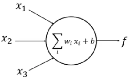
Every neuron has two types branches, the axon and the dendrites. A neuron receives input signals from its dendrites and it outputs signals using its axons. Branches of axons are then connected to dendrites of other neurons. In a similar way, the artificial neural network also consists of millions of neurons and it models biological neuron with the help of weight, bias and activation function. Fig. 2.1 describes single neuron in an artificial neural network.

This neuron receives 3 inputs x1, x2 and x3 and computes activation function f = P

wixi +b, where wi corresponds to the ith weight and b corresponds to the bias of that neuron. one of the common activation function which is used in neural networks is the sigmoid function, as expressed mathematically in equation (2.1). The sigmoid function takes the real valued number and converts it to a value within 0 and 1.

σ(x) = 1

1 +ex (2.1)

Another activation function which is often used in the neural network is the hyperbolic tangent function as shown in equation (2.2). It constrains input signal in the range of -1 to +1.

tanh(x) = e

x_−e−x

ex_+e−x = 2σ(2x)−1 (2.2) In recent years, Rectified Linear Unit (ReLU) has become one of the popular ac-tivation function in the deep neural network. ReLU function is represented as shown in the equation (2.3). ReLU function is not continuously differentiable or bounded, unlike sigmoid and tanh functions. It works better in deep networks because it expedites stochastic gradient descent convergence when compared to sigmoid and tanh function.

f(x) =max(0, x) (2.3)

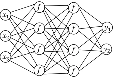
A generic neural network model is shown in Fig. 2.2. It consists of an input layer, an output layer and a number of hidden layers. Every neuron receives an input, it performs dot product between input and its weights, adds the bias and applies an activation function and sends the output to other neurons. Input layer receives

input data, each neuron in the input layer does the same processing and sends the output to the first hidden layers. The Hidden layer does the same processing and sends the output to next hidden layer. This process is repeated until the rightmost layer, also called as output layer is reached. At the output layer, scores for each class is computed and the object is classified, with the highest score representing the class of input image. The entire process of beginning from the input layer to converting signals into output score is called forward propagation.

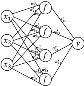
Figure 2.2: Forward Propagation

In this example of forward propagation model, the leftmost layer is an input layer, the rightmost layer is an output layer and the model has only one hidden layer in between input and output layer. Weights corresponding toith _{hidden layers} are denoted as wi

mn, where mcorresponds mth neuron in the previous (i−1)th layer and n corresponds to nth neuron in the current ith layer. Every neuron in the ith hidden layer has its own bias bi_n. Activation from every neuron in the hidden layer is calculated as shown in the equation (2.4), (2.5), (2.6) and (2.7).

ay₁₁=f(w1₁₁x1+w211 x2+w311 x3 +b11) (2.4)

ay₂₁=f(w1₁₂x1+w221 x2+w321 x3 +b12) (2.5)

ay₃₁=f(w1₁₃x1+w231 x2+w331 x3 +b13) (2.6)

ay₄₁=f(w1₁₄x1+w241 x2+w341 x3 +b14) (2.7)

In training of neural network, after the forward propagation, the loss or cost is calculated, which is the difference between predicted output score and ground truth table. In the training process, the next step is to tweak weights and biases so that the loss is minimized. This process is called optimization. The gradient of the cost with respect to weights and biases gives the rate at which weights and biases should be changed. The process of computing gradient of the cost with respect to weights and biases in the entire network is called backpropagation. The gradient is computed repeatedly and parameters are updated accordingly. This process is also known as gradient descent. In the backpropagation, the gradient at every neuron is calculated using the gradient chain rule going from output layer backward to input layer.

There is another kind of parameters called hyperparameters involved in machine learning. They decide higher level settings of neural network model such as rate of change and complexity of the model. One of the common hyperparameters used in deep neural networks is a learning rate. Learning rate decides the step size for the parameter update along the direction of the gradient. Learning rate has to be chosen carefully because if learning rate is too small, the convergence of the network for finding suitable weights will be slow and if it is too large, it may give us higher loss because of the less precision in step size.

2.2

Convolutional Neural Network

The convolutional neural network works on the same principle of the neural network. These nets also have an input layer, an output layer, and a number of hidden layers. Similar to any other neural network, every neuron in the convolutional network receives input data, it performs dot product between input data and weights, adds the bias, applies the activation function and sends the output to other neurons. The output from one layer is used as input to the next layer. At the end of propagation, scores of the classes are computed similar to any fundamental neural network. The concepts of backpropagation also remain the same in the convolutional network. The main difference between convolutional neural net and any other neural net is that convolutional neural net takes advantage of the fact that input consists of images, by arranging its neuron in 3 dimensions corresponding to width, height, and depth of the input image. In fact, the convolutional neural net can be used on any data which can be arranged in the form of spatially correlated structures such as images. In other words, if the available data is represented in the form of image structure such that spatially closer information is more related to each other than spatially farther information, the convolutional neural net can classify pattern among such data with good accuracy.

2.2.1

Convolutional layer

The convolutional layer is the core building block of the convolutional network. Neurons in this layer are not connected to every neuron in the previous layer. In-stead, every neuron is connected to the local region in the previous layer. Neurons in the convolutional layer are like a set of filters. Every filter is very small along the width and height, but every filter extends along the full depth of the input

acti-vation. During forward propagation, every filter slides across the entire image, and performs convolution between filter elements and the corresponding local regions in the input activation and produces two-dimensional output activation which is the convolutional output of the filter at every spatial position of the input activation. When filter slides across the image, it gets activated, when it is convolved with the certain type of image features such as line, curve, edge, corner or a certain combi-nation of colors. Every filter tries to identify different features from given input and stores the result in one 2-D activation map. N number of filters generates N 2-D feature maps. These N feature maps are joined along the depth to make one 3-D output activation map, which is then used as input for the next layer.

In other words, convolutional layer receives input feature map and weights for that layer and it performs the 3-D convolutional operation, as described mathemat-ically by equation (2.8). Y[n, i, j] = D−1 X d=0 K−1 X y=0 K−1 X x=0 W[n, d,2−x,2−y]∗X[d, i+x, j+y] (2.8)

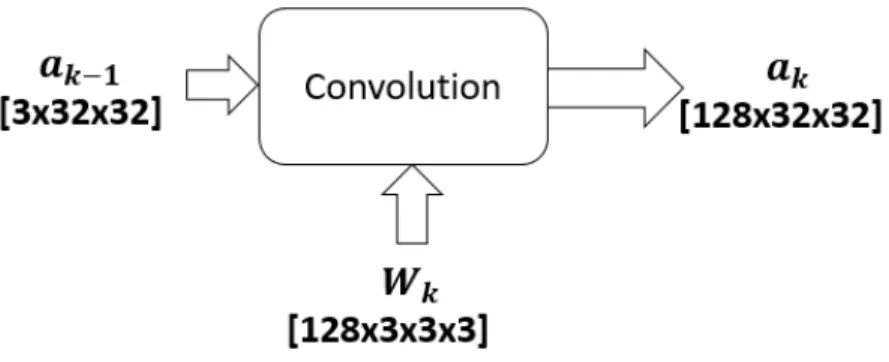
In this expression, input feature map is of size D×W ×H and output feature map is of size N ×W ×H, where N is the number of feature maps. K×K is the kernel size. Above expression gives(i, j) the value of nth _{feature map. For example,} in our first layer implementation, input feature map is an image of size 3×32×32 and the kernel is of size 3×3 and there are 128 weights of size 3×3 and depth 3, which then generates output feature map of size 128×32×32. This convolutional operation is shown in Fig. 2.3.

Important hyperparameters in the convolutional layers are a number of filters, the size of the filter, stride, and zero-padding. The number of filters corresponds to the depth of the output activation. Each filter looks for some different visual feature

Figure 2.3: First Convolutional Layer Operation

in the input. A number of filters determine the number of features that convolutional layer is extracting. The size of the filter is also called as the receptive field of the neuron. It can be anything like 3×3, 5×5, 7×7 etc. The size of the filter is always smaller in width and height as compared to width and height of input activation. But, depth of the receptive field is always same as that of input activation. Stride controls how the filter slides across the input volume. Stride decides the amount by which filter shifts. If the stride is 1, then the filter shifts every time by one pixel. If the stride is 2, then the filter shifts by 2 pixels every time. The amount of stride also determines how much output volume would shrink. If the stride is increased, then overlap between two adjacent filters decreases. Zero padding is basically used to control the size of output activation with respect to input activation.

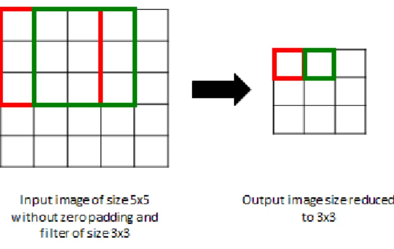
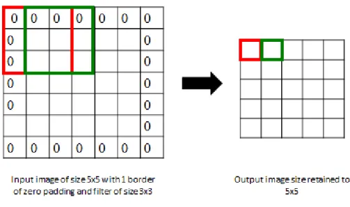
For example, consider if we have 32×32×3 input image, if we use a filter of size 3×3×3 with a stride of 1 without zero padding, it would give output activation of 30×30×3. Thus, the output volume has shrunk. If it is necessary to keep the output activation size same as the input activation, zero padding of one border can be used. Then, it would keep the output activation size to 32×32×3. Figure 2.4 and 2.5 demonstrate the significance of zero padding and stride with 2-D input and output activations

Figure 2.4: Image size reduces with 3x3 filter size without zero padding and 1 stride

2.2.2

Pooling Layer

Another layer, which is often used in between successive convolutional layers is a pooling layer. Pooling layer is used to reduce the spatial dimension of input activation layer. There are different kind of pooling layers used such as average pooling layer. In this paper, max pooling layer is used to reduce the dimension of input activation by applying simple maximum function. The example of max pooling layer application is shown in the Fig. 2.6.

Important hyperparameters involved in pooling layer is window size and window stride. The window of constant size is applied to each 2-D map in the input acti-vation independently and maximum operation is carried out. Figure 2.6 shows an example of max pooling, where window size was 2×2 and stride was 2. Pooling reduces dimension of input image from 4×4 to 2×2. Reduction in spatial dimen-sions reduces the number of parameters required in the next convolutional layers, which in turns, reduces memory requirement and computation cost for next convo-lutional layers. Additionally, pooling layer also helps in controlling overfitting. In the case, when trained neural network gives very good accuracy on trained data, but

Figure 2.5: Image size is retained with 3x3 filter with 1 border of zeros padding and 1 stride

Figure 2.6: Pooling Layer Operation

gives a way lesser accuracy for test data, that occurrence is referred as overfitting of the neural network. Applying pooling layer in between other neural network layers provides distortion and scale invariance which helps in controlling overfitting.

2.2.3

ReLU Layer

The non-linear activation function is applied after almost every convolutional and fully connected layer in most of the neural networks. There are different types of

tant non-linear functions are discussed in Section 2.1. Rectified Linear Unit function has been proven to give better results in the neural network than other non-linear function[14], because it requires lesser computational time and it also gives perfor-mance improvement when used along with some regularization scheme like dropout [15]. Regularization schemes are used to control overfitting of the neural network. In the dropout, during the training process, randomly some activation units are set to zero. This breaks up the co-adaptation of units, which results in preventing overfitting.

2.2.4

Fully Connected Layer

Each neuron in the fully connected layer has connections to all the neurons in the previous layer. However, the fully connected layer does not take into account spatial properties of images. Fully connected layer converts a list of the feature maps into a list of class scores. So, there can’t be any convolutional layer after fully connected layer. The Fig. 2.7 shows an example of several fully connected layers connected to each other. Hyperparameter involved in fully connected layers is a number of neurons in the fully connected layer. Generally, a stack of fully connected layers is used at the end of the neural network.

2.2.5

Backpropagation and Fradient Descent

Backpropagation is a common method [16] which is used along with some opti-mization method such as gradient descent to train the neural network. In other words, backpropagation is a way by which weights and biases in the convolutional and fully connected layers are adjusted so that neural network is trained to identify a particular object. When training the neural network for the first time, weights are randomly initialized. In the forward propagation, image from training dataset is

Figure 2.7: Fully Connected Layer Structure

passed through neural network to generate the class score with the randomly initial-ized weights. Then, the loss function is calculated by comparing generated output with the targeted output. The loss is usually high for the first couple of training data. The aim of backpropagation is to minimize the loss by tweaking the weights and biases.

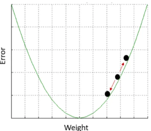
To find the direction in which weight should be changed to minimize the cost, the gradient of loss function with respect to that weight is calculated. Thus, in the backpropagation, the gradient of loss function with respect to every weight is computed using the chain rule. Once derivatives with respect to every weight are computed, then weights are changed in the direction of gradient descent. This last step is referred as parameter update. Gradient descent process is depicted in the graph as shown in Fig 2.8, where weight is adjusted down in the direction of the gradient to minimize the error.

Figure 2.8: Gradient Descent Graph of Error vs Individual Weight

The hyperparameter involved in the backpropagation is the learning rate (η). The choice of the learning rate decides how far along the gradient direction, weight should change. Learning rate is a tricky parameter and should be chosen carefully. Because, if learning step is too high, then bigger steps are taken in parameter up-date and the network will converge fast, but this also could result in insufficient precision to reach the optimal value of weight or it could lead to higher loss due to overstepping. If learning rate is too slow, that means weight training will be slower. The network will take more time to reach to the optimal values of weight.

2.3

Related Work

Simonyan and Zisserman investigated the performance of the convolutional network by increasing the depth of the network [17]. They have shown that by increasing depth of the convolutional network to 16-19 weight layers, the performance of the network can be increased substantially. But, with increasing depth of convolutional layers, computational cost and memory requirement of the neural network also in-crease. Graphic processing units (GPUs) have become solutions to implement con-volutional nets at high speed and to meet such heavy computational requirements

[18]. However, for many real-time embedded applications, high power consumption of GPU is not feasible. For low-power neural network applications, implementation of the pre trained convolutional neural network on embedded FPGA is a promising solution. But, FPGAs have limited on-chip memory resources. Thus, implemen-tation of all of the convolutional network will require external memory to store pre-trained weights and biases. But, even if the external memory is used, the lim-ited bandwidth of FPGA could lower the speed of the neural network. This makes the state of the art convolutional nets unsuitable for real-time embedded systems such as robots and automated driverless cars. To compensate for limited comput-ing and memory resources of the real-time embedded system, many researchers have proposed convolutional nets acceleration techniques on different hardware platforms. In the Farabet’s paper [19], he presented performance comparison between CPU, FPGA, and ASIC for computation of convolutional neural network. He used a neural network composed of 3 convolutional layers and 2 pooling layers. His results dictate that his convolutional system is capable of running in real-time on FPGA and ASIC with the performance better than CPU. Additionally, with ASIC and FPGA, he reported very low power consumption as low as 1W and 15W respectively.

In Dundar’s paper [20], he proposed memory access optimization scheme for convolutional neural network implemented on real-time hardware accelerator. At the input of the deep convolutional network, 3D input has to be passed to the hardware accelerator for convolution operation. However, due to the bandwidth limitation of the hardware accelerator, streaming of entire input data in and out is limited. In this paper, weight and node parallelism which occurs in 3D convolution is exploited. In his work, processes are scheduled in the hardware accelerator to calculate partial multiple outputs instead of one output. This allows optimization of hardware resources by utilizing all the available hardware resources. This achieved

110% better performance than when the routing scheme was not used.

Jiantao Qiu in his paper [21] evaluated different data quantization techniques. When the VGG16 model was used for convolution, he got only 0.4% accuracy loss with 8/4 bit dynamic precision quantization as compared to 16-bit quantization. 8/4 bit quantization also reduced three-fourths memory footprint and increased bandwidth significantly as compared to 16-bit quantization. This paper also pro-posed convolutional neural network accelerator design. This design was verified on VGG16-SVD neural network model and achieved system performance of 136.97 GOP/s.

Recently, Daniel Soudry developed Expectation Backpropagation, an algorithm using which multilayer neural network can be trained without tuning learning pa-rameters such as learning rate an can be made insensitive to the magnitude of the input. Additionally, they restricted weights to have discrete values. This makes them useful for implementing multi-layer neural network on embedded hardware with low precision. When tested on deep neural networks, Expectation Backpropa-gation outperforms the standard backpropaBackpropa-gation with optimal learning rate. They achieved the best performance using Bayes estimate of the output multi-layer neural network with binary weights.

In the recent papers by Hwang and Sung [22, 23], they proposed a technique to use lower precision weights and lower precision signals to implement the deep neural network. In their proposed method, initially trained floating point weights are trained to obtain fixed point weight directly. But, direct quantization for fixed point network does not produce good results. Thus, they proposed weight quantization strategy to retrain weight after direct quantization using backpropagation based retraining. Their fixed point network with ternary weights (+∆,0 and −∆) showed negligible performance loss when compared with the network with floating point

weights.

Courbariaux in 2015 proposed BinaryConnect method [24], which allows the deep neural network to be trained and tested with binary weights. Arithmetic operations, which are involved in deep learning are mainly convolutions and ma-trix multiplications. The most repetitive arithmetic operation in deep learning is accumulate operation. Because each neuron is nothing but a multiply-accumulator. BinaryConnect method constraints weights to be either +1 or -1. As a result, all the multiply-accumulate operations are replaced by series additions and subtractions. This brings great benefit when implementing neural network on spe-cialized hardware by removing the need of around 2/3 of multiplications. Around 1/3 of multiplications are still required while updating parameters in backpropa-gation. Because good precision weights are required to apply stochastic gradient descent for updating parameters. However, since around 2/3 of multiplications can be replaced by fixed point adders, this method can bring benefits in terms of area and power efficiency, when implementing neural network on specialized hardware platforms.

Later in 2016, Courbariaux proposed binary neural network [1], which is a convo-lutional neural network with binary weights and activations. During training binary neural network, he used binary weights and activations to compute parameter gra-dients. These parameter gradients are then used to update weights to minimize loss function. During the testing phase of the binary neural network, he used binary weights and activations to generate the class score. To analyze binary neural net-work, two different frameworks, Torch7 and Theano were used. When tested on three different datasets, CIFAR-10[5], MNIST[25] and SVHN[26], the binary neural network showed small accuracy loss as compared to state of the art results. More details about the working of the binary neural network are given in the next section.

2.3.1

Binary Neural Network[1]

In the binary neural network, weights and activations for each of the convolutional layer are constrained to be either +1 or -1. To transform floating point weights and activations into these two binary values, two different binarization methods are proposed by Courbariaux. One of them is deterministic binarization method, which is a simple sign operation as shown in equation (2.9), where x is the floating point number and xb is the binarized variable of x.

xb =sign(x) =        +1 x≥0 −1 otherwise (2.9)

Another way to binarize floating point weights is stochastic binarization as shown in the equation (2.10). This is a more precise way of binarization than deterministic binarization. xb =        +1 with probability p=σ(x) −1 with probability1−p (2.10)

whereσis the hard sigmoid function, computed as shown in the equation (2.11).

σ(x) =clip(x+ 1

2 ,0,1) = max(0, min(1, x+ 1

2 )) (2.11)

For implementing binarization on hardware, deterministic binarization is re-quired less computation and less memory space. Because stochastic binarization requires hardware to generate random bits while quantizing. Additionally, results are comparable in both cases. Thus, the deterministic method is chosen in this

Figure 2.9: Example of Binary Neural Network thesis.

Forward and Backward Propagation

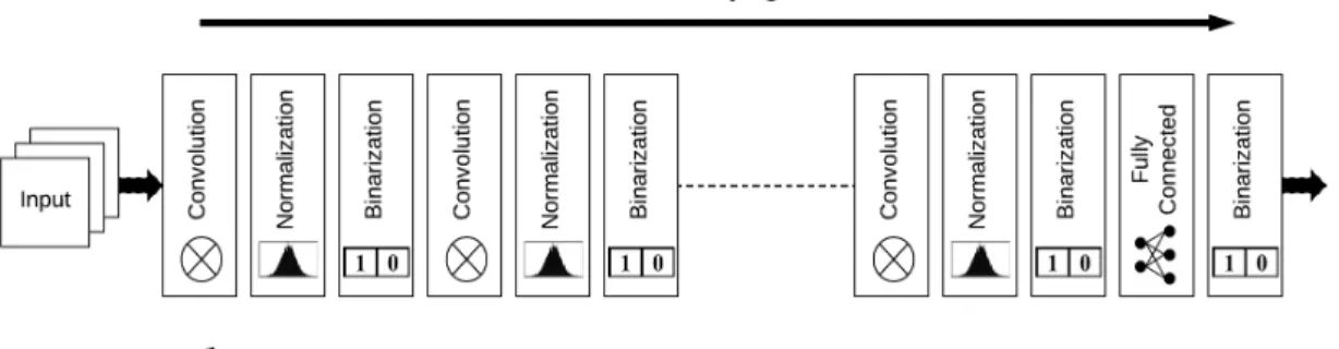
The binary neural network consists of convolutional layer, batch normalization layer, pooling layer, binarization layer and fully connected layer. The example of a binary neural network is shown in the Fig. 2.9.

Using the forward propagation, only binary weights are used for convolutional and fully connected layer. The output from one layer is connected as an input to another layer. For the first convolutional layer, the input is 8 bit fixed point value from each of the red, green and blue channels of colored image input. Thus, convolution is performed between 8 bit fixed point input and binary weight of the first convolutional layer. Since one of the arguments in the convolution is constrained to be either +1 or -1, multiply-accumulate operations in the convolution are replaced by series of additions and subtractions. For example, if x is the 8 bit fixed point input and wb is the binary weight corresponding to that input, output terms for that multiplication can be computed as shown in the equation (2.12).

s=

8

X

n=1

2n−1(x[n−1]·wb) (2.12)

wherex[7]will be most significant bit of inputx. Sincex[n] value is a binary num-ber and wbis either +1 or -1, convolution is performed by simple additions and/or subtractions. Thus, convolution performed at every neuron in the first convolu-tional layer is basically series of additions and subtractions. For all the remaining convolutional layers, input activations are binarized and weights are also binarized. Thus, all the multiply-accumulate operations will be XNOR-addition operations. This makes the computation simpler than in the case of first convolutional layers. Similarly, for fully connected layers all the arithmetic operations are replaced by bit-wise operations. Pooling layers are not shown in the Fig. 2.9. But, they are inserted at regular intervals in the binary neural networks to reduce the spatial dimension of activations.

Once the forward propagation is completed and loss is computed, gradient with respect to every parameter is calculated by moving backward in the binary neural network. The real-valued gradients are calculated because the good precision of gradients is required for Stochastic Gradient Descent (SGD) process [27]. SGD is an optimization algorithm for deep learning. SGD typically uses smaller learning rate. SGD takes small noisy step sizes in modifying the parameter until it reaches the optimized parameter value. The real-valued gradients are added to real-valued weights to compute updated weights as shown in the equation (2.13).

wt=clip(wt−1−η ∂c ∂wb

) (2.13)

where,wt−1is the old real-valued weight,ηis the learning rate, _∂w∂c

b is the gradient

clipped to be in the range of -1 to +1. Because, if the weight is beyond the range of -1 to +1, it may grow very large with each weight update. Since binarization anyways constrains the weight to be in the range of -1 to +1, the larger magnitude of weights will not affect the neural network.

The one issue with the sign function is that derivative of sign function is always zero. This causes a problem in backpropagation. While propagating backward, gradients are calculated using the chain rule. When the gradients of the cost with respect to weights are computed, sign function makes gradients to be zero. This is harmful in network learning process. Hinton introduced straight through estimator in 2012 [28], which can be used here to solve zero gradient issue. Straight through estimator applies simple hard threshold function to calculate the gradient. For example, consider sign quantization function, y=sign(x). g is computed as shown in expression (2.14). Straight through estimator performs backpropagation through sign function by treating derivative of sign function as an identity function. This cancels the gradient, only whenxis too large. Straight through estimator has proven to give good results [28] and it is simpler to implement in hardware.

gx =        gy |x| ≤1 0 otherwise (2.14)

Chapter 3

Hardware Implementation

3.1

FPGA Overview

Field Programmable Gate Arrays (FPGAs) are semiconductor devices, which can be electrically programmed to implement any digital circuit. FPGA consists of an array of programmable logic blocks, which are linked using programmable interconnects. Their reconfigurability distinguishes them from Application Specific Integrated Cir-cuits (ASICs), which are custom build for a specific design. Similar to ASICs, FPGA designs are modeled using Hardware Description Languages (HDLs) like Verilog and VHDL. Once the design is described in HDL, then it is compiled and implemented to create a configuration file, also known as bitstream file. This bitstream file contains information about how different components of FPGAs should be wired. Once this bitstream file is downloaded on FPGA, it is configured to run the design until the FPGA is powered off.

From the very beginning, when FPGAs were introduced, they have become a popular choice for engineers to prototype ASICs, ASSPs, and SoCs design to test various aspects of design. The main reason behind this is their reconfigurability. If

the design is found to be faulty, then the design can be corrected just by changing the HDL code and downloading new bitstream onto FPGAs. Being re-configurable, FPGAs can always keep pace with future modification. Another major advantage of FPGA is the time taken to fully develop a functional design. A design can be made functional and verified for different cases on FPGAs without going through long fabrication process and unusual silicon respins of custom ASIC design. FPGAs are often used to demonstrate an idea to customers and to give them assurance that the design is functioning as expected. Parallel processing allows FPGAs to build complex designs with multiple parallel executions. They used as accelerators along with CPUs in my applications because unlike CPU they can execute multiple instructions at the same time giving very high throughput. FPGAs do have some disadvantages over ASICs such as reconfigurability of FPGAs make them slower in clock speed than ASICs because ASIC designs are optimized for a specific design to get the best routing and interconnection for that design. Power consumption in FPGA designs is more as compare to custom ASICs. FPGAs have limited resources. Overall, FPGAs are preferred for lower speed designs and for lower quantity produc-tion. Additionally, FPGAs also have special in-built hardware such as block RAMs, digital clock managers, high-speed I/Os, soft-core embedded CPU, DSP blocks etc., which can be used to built almost any type of design.

3.2

ZYNQ ZC706 FPGA Platform

In this thesis, Xilinx ZC706 evaluation board is used to implement neural network. The ZYNQ 7000 family is based on Xilinx All Programmable SoC (AP SoC) archi-tecture [2]. The ZYNQ 7000 AP SoC combines the software programmability of the ARM-based processor with hardware programmability of FPGA along with CPU,

DSP, ASSP and mixed signal designing on a single silicon. ZC706 board has dual core ARM cortex-A9 processor as the heart of the processing system and 28 nm fabrication technology based ZC7Z045 FPGA as a heart of programming logic. Fig. 3.1 shows ZC706 FPGA board and its different parts. The processing system also includes on-chip memory, external memory interfaces, 8-channel DMA controller, a variety of I/O peripheral interfaces. Programming logic mainly consists of config-urable logic blocks (CLBs), Block RAMs (BRAMs), Digital Signal Processing blocks (DSP blocks), programmable I/O blocks, PCIe blocks, high-speed transceivers and Analog to Digital Converters (ADCs). For this thesis, we used Vivado 2015.2 en-vironment for rapid development of hardware and software designs. A broad range of IPs, provided by Xilinx and other 3rd party companies are used to simplify the process of designing.

Figure 3.1: ZC706 FPGA Platform[2]

Dual core ARM based processing system, on-chip memory or DDR, I/O pe-ripherals and programmable logic are connected to each other via ARM AMBA

AXI interconnects. AMBA AXI interconnect supports multiple master-slave trans-actions. This interconnect is designed in such a way that it provides the shortest path from latency sensitive ARM CPU to memory and it provides high throughput connection from bandwidth critical master such as programmable logic to its slaves. ZC7045 has up to 8 clock management tiles (CMTs), each consisting of one mixed mode clock manager (MMCM) and one phase locked loop (PLL). Both of them are used as frequency synthesizers to generate a wide range of frequencies. They also act as jitter reducers for incoming clocks.

3.3

Avnet HDMI Input Output FMC Module

The FMC-HDMI-CAM-G [3] is a low pin count (LPC) FPGA mezzanine card (FMC). This module itself doesn’t have processing intelligence. It is rather a plug-in module, compatible with FPGA platforms with LPC connector. In this thesis, FMC HDMI CAM is used along with Xilinx ZC706 FPGA platform for interfacing video input and output. Carrier board ZC706 received video data from FMC-HDMI-CAM-G board. ZC706 provides data, control and power processing for this FMC module. Fig. 3.2 shows the architecture of FMC-HDMI-CAM-G module.

Either HDMI input port or camera can be selected as a video input and video output is connected to HDMI output port. HDMI input port has ADV7611 integrated circuit as HDMI receiver and HDMI output port has ADV7511 integrated circuit as HDMI transmitter. The FMC module supports video input and output transmission in YCbCr 4:2:2 format. It supports a variety of resolution at the HDMI input as shown in the Table 3.1.

Resolution Pixel Rate Frame Dimension Frame Rate

1080P60 148.5 MHz 1920 x 1080 60 Hz SXGA 110 MHz 1280 x 1024 60 Hz 720P60 74.5 MHz 1280 x 720 60 Hz XGA 65 MHz 1024 x 768 60 Hz SVGA 40 MHz 800 x 600 60 Hz 576P50 27 MHz 720 x 576 60 Hz 480P60 27 MHz 720 x 480 60 Hz VGA 25.175 MHz 640 x 480 60 Hz

Table 3.1: Resolutions supported by HDMI Input Output FMC Card [3]

3.4

Binary Neural Network Hardware

Implemen-tation

In this thesis, GPU is used to train the neural network with binary weights and acti-vations. During training time, real time weights and real-time parameter gradients are used to perform parameter updates. Once the training is finished, updated real time weights are converted into the binary form using deterministic binarization and then pre-trained weights are stored in the on-chip memory of an FPGA. Since all the pre-trained weights are in binary format, this step saves the significant amount of memory. Since now, instead of 8 bit/16 bit weights, 1-bit weights are saved into the on-chip memory of FPGA, memory usage reduces by 8/16 times.

The small BNN architecture implemented on ZYNQ ZC706 platform is as shown in figure 3.3. This architecture consists of only 2 convolutional layers and 3 fully connected layers.

Figure 3.3: Architecture of Binary Neural Network

For the first layer of BNN, input is CIFAR-10 RGB image of dimensions 3×32×32 and each pixel is of 8-bit precision. Since weights to this layer are binarized, the convolution operation is no longer multiply accumulations. Instead, it will be series of addition (when corresponding weight is +1) and subtraction (when corresponding weight is -1). Then, equation (1) for convolution can be rewritten as in (3.1), where Wb =sign(W). In other words, Wb is the stored binary weight obtained by binarizing real time weight W.

Y[n, i, j] = D−1 X d=0 K−1 X y=0 K−1 X x=0 Wb[n, d,2−x,2−y]∗X[d, i+x, j+y] (3.1)

Input for testing phase is an image of size 32×32×3. An image is sent to the binary neural network through AXI4-Stream interface. Each pixel in R, G and B components of images of 8-bit size. Thus, the data width of AXI4-Stream interface is 24 bits. The pixels are received in a raster scanning order. Output image from the

order. The kernel size of the 3D convolutional filter is 3×3×3. 3D convolution is performed by first computing 2D convolutions with kernel size of 3×3 and then adding the results from three 2D convolutions. The hardware module needs to buffer the image pixels to perform 3D convolution. To perform convolution with kernel size of 3×3, an image needs to be buffered up to at least 2 rows of the pixels. For the mask 3×3, output sample is a function of 9 pixels, each of 8 bits corresponding to the pixel in each component of RGB image. To retain width×height of output volume to be 32×32, zero padding of one order is applied to an image. With stride of 1, each pixel is read 9 times as the window is scanned through the image. Pixels adjacent horizontally are required in successive clock cycles, so are buffered and delayed in registers. A row buffer caches the value of previous rows to avoid having to read the pixel values again. A filter of 3×3 spans three rows, the current row and two previous rows as shown in Fig. 3.4. Each buffer delays the input by one row. To implement such delay, N stage shift register is used, where N is the width of the image, which is 34 in this case with 1 level of zero padding.

Figure 3.4: Line buffers to scan 3×3 pixels at a time

Architecture realization of the first layer is as shown in following Fig. 3.5. Input here is a test image from CIFAR-10 dataset of size32×32×3. This figure shows computation of N feature maps when N kernels of size 3×3× 3 convolves with RGB input image of size 128×128×3. A number of output feature maps are equal

to the number of kernels. Since Wb can only take two values +1 or -1, multiply-accumulation operations of convolution changes to series of additions (when Wb is +1) and series of subtractions (when Wb is -1) as shown in Fig. 3.6.

Figure 3.5: first convolution layer

Figure 3.6: First Convolution Layer, multiply accumulate implemented by addition subtraction

All other convolution layers except first layer have binarized weights as well as binarized inputs. Hence, the realization of all other convolution layer is same as shown in Fig. 3.7. This figure shows the computation of N output feature maps when

layer. In this realization, all the multiply operations in the convolutional layer are replaced by xnor operations. Since 2D convolution operation occupies 90% of computation cost in CNN, replacing most of the multipliers by xnor gate reduces the complexity of computations by a significant amount. In other words, replacing most of the 32-bit floating point multiply accumulations by 1-bit xnor count operations reduces hardware usage by an orders of magnitudes.

Figure 3.7: 2nd, 3rd and 4th convolution layer realization

For fully connected layers, inputs are binary feature maps from previous layers and binary weights are stored in the registers of an FPGA. Again, fully connected layers in CNN consist of mainly multiplication operations. Hence, all the multipli-cation operations in the fully connected layer are replaced by XNOR operations. The usual problem faced with the fully connected layer in any CNN model is a large number of weights, which require large memory for storage. However, in the binary neural network, since weights are binary, they are easily stored into the on-chip memory of FPGA. Full connected realizations are shown in Fig. 3.8. This figure

shows computation of output class score of N classes.

Figure 3.8: Fully Connected Layer Realization

Realization of batch normalization requires four fixed point stored parameters, µ, σ, γ, β for each of the input activation layer, according to equation (3.2) [27]. In this expression, x is the input data , y is the output data. During traing,µ and σ2 are mean and variance of current input minibatch x, and during testing they are replaced by avreage statistical mean and variance over training data.

y= √x−µ

σ2₊γ+β (3.2)

However, in binary neural network implementation, we have reduced requirement of stored parameters to two (one fixed point parameter and one binary parameter), for each input activation layer. This is possible due to shifting and scaling of ex-pression (3.2) to (3.3), as follows. After every batch normalization operation, sign function is applied to quantize input to the value of +1 or -1. We have taken

ad-vantage of this, by neglecting magnitude of scaling function _βγ and only storing sign of scaling function as a binary parameter. Because only sign of the scaling func-tion will have a contribufunc-tion in quantizing final batch normalized output. In our implementation, we have batch normalization layer after every convolutional and fully connected layer. By using this shift and scale operation, now memory require-ment for storing batch normalization parameter reduces from 32 bits (8 bits * 4 parameters) to 9 bits (8 bit + 1 bit), for each activation layer.

y=qb(x+p) (3.3) where p= βσ γ −µ , q = γ σ and qb =sign(q)

3.5

Top Level System Design

Avnet HDMI I/O FMC module is connected to Xilinx ZC706 platform via LPC connector. Input video stream of 720p at 60 fps is given to HDMI input port of Avnet HDMI I/O FMC. Avnet FMC has ADV7611 IC integrated on it, which receives an incoming video signal and then pass it to programmable logic design for further processing. In programmable logic design, video input is converted into AXI4-Stream format using Video In to AXI4-Stram IP provided by Xilinx. The video is in YCbCr 4:2:2 format when streamed out of this IP. Chroma Resampler IP and YCbCr to RGB Color Space Converter IP is used to convert YCbCr 4:2:2 video into RGB 4:4:4 format pixel by pixel.

AXI4-Stream interface streams one pixel per clock cycle. It has different signals for tracking positions of input frame pixels. Some of the common AXIS signals are data signal of 24-bit width, start of frame (SOF), end of line (EOL), valid signal

Figure 3.9: Example of AXI4-Stream interface transmission [4]

and ready signal. SOF signal is active high for every first pixel of the video frame. It acts as a frame synchronizer for all of the cores streaming in AXIS video input. EOL signal marks the last pixel of every scanned line. The valid signal is active high for every active high video data. Ready and valid signals are used together for handshaking, whenever data is transmitted between 2 IP core. An example of AXIS interface signals is shown in the form of the waveform in Fig. 3.9.

Once the video is converted into RGB AXI4-Stream format, an encoder is used to store exactly 32×32 pixels each of 24 bit width out of 720p frame inside dual port block RAM. At the same time, a decoder is used to read the data stored in block RAM. The data read by the decoder is used as input for binary neural network module. Neural network uses pre-trained weights stored into registers of FPGA and pass 32×32 RGB frame through several layers of neural network and outputs one bit determining whether the class is detected or not. The output is synchronized with input video stream to send signal whether the particular object is detected or not. This system is shown in Fig. 3.10. Output AXI4-Stream is then again converted to YCbCr 4:2:2 format using proper IPs and then to appropriate video format and transmitted out from Avnet FMC HDMI output port for displaying.

Chapter 4

Classification and Result

4.1

BNN Classification Result

The CIFAR-10 dataset is used for training and testing binary neural network for automobile classification. All the images in the CIFAR-10 are 32×32 color images. CIFAR-10 dataset can be distinguished into 10 different classes. Some examples of images from every class in shown in the following Fig. 4.1.

50,000 images are used to train binary neural network on GPU. The distribution of the images is such that 5,000 images belong to every class. The testing dataset contains 10,000 images with exactly 1,000 randomly ordered images belonging to every class. The proposed design of the neural network is trained and tested for automobile classification.

The architecture used for binary neural network layer is inspired by convolution neural network of VGG Net [29]. When 1-bit binary weights are used in the convo-lutional network instead of fixed point representation, the memory required to store weights decreases by an order of magnitude. In addition to that, resources required to conduct the multiplication-addition operation at every neuron also reduces by a significant amount. Furthermore, if input activations are quantized to 1 bit along with weights for convolutional and fully connected layers, complex arithmetic op-erations are replaced by bitwise opop-erations leading to further decline in resource usage.

For an instance, consider a case when input activation for a convolutional layer is of size 32×32×16 and neurons have a receptive field of size 3×3×16 with depth 16, sliding with stride 1. Input activation is surrounded by one layer of zero padding. Then, the output volume would be of size 32×32×16, same as input activation. In other words, this is the case of convolutional layer with 32∗32∗16 = 16,384 neurons, each having 3∗3∗16 = 144 weights. Table 4.1 shows resource utilization on Virtex -7 FPGA when this convolution layer is implemented. For implementing this convolutional layer, weights and activations are defined to be of fixed point 8 bits.

To carry out 8-bit multiplications at every neuron, DSPs are employed. All other connections are realized using registers and LUTs. When the same convolu-tional layer is implemented using binarized weights and 8-bit activations, resource

Resource Utilization Available Utilization%

Slice Registers 22016 607200 3.63

Slice LUTs 24263 303600 7.99

DSP48 2304 2800 82.29

Table 4.1: Resource utilization, when weights and activations are of fixed point 8 bit

utilization is as shown in Table 4.2.

Resource Utilization Available Utilization

Slice Registers 8592 607200 1.42

Slice LUTs 8698 303600 2.86

Table 4.2: Resource utilization, when weights are binarized and activations are of fixed point 8 bits

Since now all the weights are binarized, DSPs are no longer needed to carry out multiplications at every neuron. Because one of the arguments of multiplication is binarized (+1 or -1) and other is of fixed point 8 bit, multiply operation is no longer required. Output at every neuron can be calculated by just executing series of additions and/or subtractions. In addition to this, registers required decreases by 60.97% and LUTs required decreases by 64.15% , as can be seen from the utilization tables. Table 4.3 shows the utilization of resources when the same convolutional layer is implemented with binarized weights and binarized activations.

Resource Utilization Available Utilization

Slice Registers 2141 607200 0.35

Slice LUTs 2507 303600 0.83

Table 4.3: Resource utilization, when weights and activations are binarized

As can be seen from the table, resource usage further reduces, when both weights and activations are binarized. When both the arguments of multiplications are bi-narized, multiplication output can be carried out by using simple bitwise XNOR

duces by 71.17%, as compared to the implementation with only binarized weights. When this convolution layer implementation with binarized weights and activations is compared with fixed point weights and activations implementation, the require-ment of resources has decreased by 90.27% for registers and 89.66% for LUTs. This is a huge improvement on resource utilization. This implementation saves a good amount of FPGA resources, which can be used to implement other digital system or another network layer on FPGA.

This thesis proposes a binary neural network implementation with 5 convolu-tional layers and 3 fully connected layers. Table 4.4 shows a number of parameters required by this network architecture.

Network layer Weights required for given layer Convolutional layer 3∗3∗3∗128 = 3,456 Convolutional layer 3∗3∗128∗128 = 147,456 Pooling layer 0 Convolutional layer 3∗3∗128∗256 = 294,912 Convolutional layer 3∗3∗256∗256 = 589,824 Pooling layer 0 Convolutional layer 3∗3∗256∗512 = 1,179,648 Pooling layer 0

Fully connected layer 4∗4∗512∗1024 = 8,388,608 Fully connected layer 1024∗1024 = 1,048,576 Fully connected layer 1024∗10 = 10,240

Table 4.4: Parameters required by each layer of proposed network

When the parameters required for all the layers are added, total number of parameters would be _∼ 11.6M illions. If this architecture is implemented with convolutional layers with fixed point 8-bit weights, then memory required would be 11.6M B. On the other hand, if this architecture is implemented with binary neural network with binarized weights, memory required would be 11.6M/8 =_∼145.7KB. Thus, binary neural network reduces memory requirement by 98.75%.

Virtex-7 980T FPGA platform. Xilinx Vivado 2015.2 environment is used to perform synthesis and implementation on the design. Mainly registers and LUTs are used in this design. Table 4.5 shows resource utilization when the binary neural network is implemented with a different number of layers.

no. of convolution layers 1 2 3 4 5

no. of fully connected layers 1 1 2 2 3

Slice Registers 24195 178391 213095 350713 499874

Slice LUTs 3563 507905 650126 888927 1113205

Table 4.5: Resource utilization, when number of convolutional and fully connected layers are varied in the network

When a binary neural network with 5 convolutional layers and 3 fully con-nected layers is implemented on Virtex-7 980T FPGA, maximum frequency of 340.13M Hzis recorded. When tested on CIFAR-10 test dataset, the accuracy achieved is 86.06%. This neural network also has several pooling layers and a batch normalization layer after every convolutional and fully connected layer. Total la-tency of this system is 1670 clock cycles or 4.9µs. Maximum throughput of this design can reach is 332,164 images per second with 32×32 resolution.

Chapter 5

Conclusion and future work

5.1

Conclusion

Over the last few years, Advanced Driving Assistance System (ADAS) is one of the fastest evolving research division in academia and automobile industry. The aim of ADAS is to provide assistance to the driver by alerting him about the poten-tial danger and reducing chances of accidents due to driver’s negligence. Accurate environment perception is essential for ADAS implementation. One of the key tech-nology involved in environment monitoring is computer vision. Computer vision is useful in a variety of applications of ADAS such as lane detection, road sign detec-tion, vehicle detecdetec-tion, automotive cruise control and driver monitoring. To address all these different applications, various computer vision algorithms are studied and discovered. Among those, the deep convolutional neural network has achieved break-through results in the field of image recognition in last few years. The convolutional neural network was then followed by many other modified networks for improving performance further or to make network optimized for specific pattern recognition problem. The binary neural network is one of those modified convolutional

neu-ral network designed to address pattern recognition problems for real-time and low power embedded applications.

In this thesis, FPGA-based SoC design for the binary neural network is pro-posed. Since FPGA has reconfigurable and parallel architecture, it is a powerful platform for the deep neural network. Reconfigurability of FPGA allows neural network architecture to be scalable and adaptable to change. When looked deep down, neural network is nothing but millions of neuron performing the same arith-metic operation. Since the same repetitive operation is performed at every neuron independently, parallel computing architecture of FPGA can be utilized to execute independent operations concurrently. The drawbacks of using FPGA platform are limited on-chip memory size and limited bandwidth if the external memory is used for storing weights. Since FPGA implementation of binary neural network uses pre-trained binary weights, storing weights into only on-chip memory is feasible and limited bandwidth is no longer an issue. This proposed architecture provides very high throughput, since there is no latency due to external memory access and limit on the external memory bandwidth. This design provides processing capacity of 332,164 images per second. This design achieved maximum accuracy is 86.06%, by optimizing usage of memory resources on the FPGA platform. Due to low power and small memory requirements, proposed design can be a suggested solution for many embedded system applications.

5.2

Future work

In this thesis, binary neural network implementation was only targeted for vehicle detection task. In the future work, the binary neural network can be used to ad-dress other real-time computer vision tasks in ADAS such as traffic sign detection,

automotive cruise control and driver drowsiness monitoring tasks.

FPGAs have parallel processing architecture. Thus, it is possible to run multiple computer vision applications of ADAS at the same time on single FPGA if there are enough computational and memory resources. Higher end FPGAs like Ultrascale family FPGAs can be employed to meet more computational and memory resource demand. With the Ultrascale family of FPGA, a deeper neural network can also be realized, which can achieve higher accuracy. In fact, FPGA can be used for entire ADAS designing, because FPGA can provide benefit from parallel processing which will be used in sensor data processing. Simultaneously, it can also be used to handle serial processing task like system control, system monitoring, alerting system etc with the help of ARM processor.

With this FPGA implementation, 86.06% accuracy is achieved for object classi-fication task with 5 convolutional and 3 dense layer architecture. ASIC implementa-tion of the same binary neural network design can further improve the performance per power consumption. Though FPGA provides an advantage of reconfigurabil-ity, ASIC will also allow more depth in the neural network, thus identifying more complex patterns efficiently with the greater accuracy.

Bibliography

[1] Matthieu Courbariaux, Itay Hubara, COM Daniel Soudry, Ran El-Yaniv, and Yoshua Bengio. Binarized neural networks: Training neural networks with weights and activations constrained to+ 1 or-.

[2] Zynq-7000 all Programmable SoC Overview.

[3] Avnet FMC-HDMI-CAM-G Hardware Design Guide.

https://www.avnet.com/shop/us/p/kits-and-tools/development-kits/avnet-engineering-services-ade–1/aes-fmc-hdmi-cam-g-3074457345628965509. [4] AXIStream Data Interface Signal Descriptions.

[5] CIFAR-10 and CIFAR-100 datasets.

[6] Geoffrey E Hinton, Simon Osindero, and Yee-Whye Teh. A fast learning algo-rithm for deep belief nets. Neural computation, 18(7):1527–1554, 2006.

[7] Yoshua Bengio, Pascal Lamblin, Dan Popovici, Hugo Larochelle, et al. Greedy layer-wise training of deep networks. Advances in neural information processing systems, 19:153, 2007.

[8] Marc’Aurelio Ranzato, Christopher Poultney, Sumit Chopra, and Yann LeCun. Efficient learning of sparse representations with an energy-based model. In

Pro-ceedings of the 19th International Conference on Neural Information Processing

Systems, pages 1137–1144. MIT Press, 2006.

[9] George Dahl, Abdel-rahman Mohamed, Geoffrey E Hinton, et al. Phone recog-nition with the mean-covariance restricted boltzmann machine. InAdvances in neural information processing systems, pages 469–477, 2010.

[10] Pascal Vincent, Hugo Larochelle, Isabelle Lajoie, Yoshua Bengio, and Pierre-Antoine Manzagol. Stacked denoising autoencoders: Learning useful represen-tations in a deep network with a local denoising criterion. Journal of Machine

Learning Research, 11(Dec):3371–3408, 2010.

[11] Alex Graves, Abdel-rahman Mohamed, and Geoffrey Hinton. Speech recog-nition with deep recurrent neural networks. In Acoustics, speech and signal

processing (icassp), 2013 ieee international conference on, pages 6645–6649.

IEEE, 2013.

[12] Alex Krizhevsky, Ilya Sutskever, and Geoffrey E Hinton. Imagenet classification with deep convolutional neural networks. In Advances in neural information processing systems, pages 1097–1105, 2012.

[13] Adam Coates, Paul Baumstarck, Quoc Le, and Andrew Y Ng. Scalable learn-ing for object detection with gpu hardware. In 2009 IEEE/RSJ International

Conference on Intelligent Robots and Systems, pages 4287–4293. IEEE, 2009.

[14] George E Dahl, Tara N Sainath, and Geoffrey E Hinton. Improving deep neural networks for lvcsr using rectified linear units and dropout. In Acoustics, Speech and Signal Processing (ICASSP), 2013 IEEE International Conference on, pages 8609–8613. IEEE, 2013.

[15] Nitish Srivastava, Geoffrey E Hinton, Alex Krizhevsky, Ilya Sutskever, and Ruslan Salakhutdinov. Dropout: a simple way to prevent neural networks from overfitting. Journal of Machine Learning Research, 15(1):1929–1958, 2014. [16] Paul J Werbos. Backpropagation through time: what it does and how to do it.

Proceedings of the IEEE, 78(10):1550–1560, 1990.

[17] K. Simonyan and A. Zisserman. Very deep convolutional networks for large-scale image recognition. CoRR, abs/1409.1556, 2014.

[18] Adam Coates, Paul Baumstarck, Quoc Le, and Andrew Y Ng. Scalable learning for object detection with gpu hardware. In Intelligent Robots and Systems,

2009. IROS 2009. IEEE/RSJ International Conference on, pages 4287–4293.

IEEE, 2009.

[19] Cl´ement Farabet, Berin Martini, Polina Akselrod, Sel¸cuk Talay, Yann LeCun, and Eugenio Culurciello. Hardware accelerated convolutional neural networks for synthetic vision systems. In Circuits and Systems (ISCAS), Proceedings of

2010 IEEE International Symposium on, pages 257–260. IEEE, 2010.

[20] Aysegul Dundar, Jonghoon Jin, Vinayak Gokhale, Berin Martini, and Eugenio Culurciello. Memory access optimized routing scheme for deep networks on a mobile coprocessor. In High Performance Extreme Computing Conference

(HPEC), 2014 IEEE, pages 1–6. IEEE, 2014.

[21] Jiantao Qiu, Jie Wang, Song Yao, Kaiyuan Guo, Boxun Li, Erjin Zhou, Jincheng Yu, Tianqi Tang, Ningyi Xu, Sen Song, et al. Going deeper with embedded fpga platform for convolutional neural network. In Proceedings of the 2016 ACM/SIGDA International Symposium on Field-Programmable Gate