Durham Research Online
Deposited in DRO:05 August 2014
Version of attached le:
Accepted Version
Peer-review status of attached le:
Peer-reviewed
Citation for published item:
Coolen-Maturi, T. (2014) 'Nonparametric predictive pairwise comparison with competing risks.', Reliability engineering system safety., 132 . pp. 146-153.
Further information on publisher's website:
http://dx.doi.org/10.1016/j.ress.2014.07.014 Publisher's copyright statement:
NOTICE: this is the author's version of a work that was accepted for publication in Reliability Engineering System Safety. Changes resulting from the publishing process, such as peer review, editing, corrections, structural formatting, and other quality control mechanisms may not be reected in this document. Changes may have been made to this work since it was submitted for publication. A denitive version was subsequently published in Reliability Engineering System Safety, 132, 2014, 10.1016/j.ress.2014.07.014.
Additional information:
Use policy
The full-text may be used and/or reproduced, and given to third parties in any format or medium, without prior permission or charge, for personal research or study, educational, or not-for-prot purposes provided that:
• a full bibliographic reference is made to the original source
• alinkis made to the metadata record in DRO
• the full-text is not changed in any way
The full-text must not be sold in any format or medium without the formal permission of the copyright holders. Please consult thefull DRO policyfor further details.
Durham University Library, Stockton Road, Durham DH1 3LY, United Kingdom Tel : +44 (0)191 334 3042 | Fax : +44 (0)191 334 2971
Nonparametric predictive pairwise comparison
with competing risks
Tahani Coolen-Maturi
Durham University Business School, Durham University, Durham, DH1 3LB, UK
Abstract
In reliability, failure data often correspond to competing risks, where several failure modes can cause a unit to fail. This paper presents nonparametric predictive inference (NPI) for pairwise comparison with competing risks data, assuming that the failure modes are inde-pendent. These failure modes could be the same or different among the two groups, and these can be both observed and unobserved failure modes. NPI is a statistical approach based on few assumptions, with inferences strongly based on data and with uncertainty quantified via lower and upper probabilities. The focus is on the lower and upper prob-abilities for the event that the lifetime of a future unit from one group, say Y, is greater than the lifetime of a future unit from the second group, sayX. The paper also shows how the two groups can be compared based on particular failure mode(s), and the comparison of the two groups when some of the competing risks are combined is discussed.
Keywords: Competing risks, reliability, pairwise comparison, nonparametric predictive inference, lower and upper probabilities, lower and upper survival functions,
right-censored data.
1. Introduction
In reliability, failure data often correspond to competing risks (Bedford et al., 2008; Ray, 2008; Sarhan et al., 2010), where several failure modes can cause a unit to fail, and where failure occurs due to the first failure event caused by one of the failure modes. Throughout this paper, it is assumed that each unit cannot fail more than once and it is not used any further once it has failed, and that a failure is caused by a single failure mode which, upon observing a failure, is known with certainty. Also we assume throughout that the failure modes are independent, inclusion of assumed dependence would be an interesting topic for future research, but cannot be learned about from the data as considered here, as shown by Tsiatis (1975).
Comparison of two groups or treatments with competing risks is a common problem in practice. For example in medical applications, one may want to compare two treatments with multiple competing risks (Luo and Turnbull, 1999), or in reliability one may want to study the effect of the brand of air-conditioning systems which can fail either due to leaks of refrigerant or wear of drive belts (Park and Kulasekera, 2004). One may wish
to compare the two groups either by taking into account all the competing risks or just considering particular competing risks. For example, when studying occurrence of cancer among men and women where cervical cancer (prostate cancer) can cause only women (men) to die and lung cancer can cause both women and men to die, so cervical and prostate cancer each are risks to only one group while lung cancer affects both groups.
In this paper we introduce nonparametric predictive inference (NPI) for comparison of two groups with competing risks. NPI is a statistical method based on Hill’s assump-tion A(n) (Hill, 1968), which gives a direct conditional probability for a future observable
random quantity, conditional on observed values of related random quantities (Augustin and Coolen, 2004; Coolen, 2006). A(n) does not assume anything else, and can be
inter-preted as a post-data assumption related to exchangeability (De Finetti, 1974), a detailed discussion of A(n) is provided by Hill (1988). Inferences based on A(n) are predictive and
nonparametric, and can be considered suitable if there is hardly any knowledge about the random quantity of interest, other than the n observations, or if one does not want to use such information, e.g. to study effects of additional assumptions underlying other statistical methods. A(n) is not sufficient to derive precise probabilities for many events
of interest, but it provides bounds for probabilities via the ‘fundamental theorem of prob-ability’ (De Finetti, 1974), which are lower and upper probabilities in interval probability theory (Augustin and Coolen, 2004; Walley, 1991; Weichselberger, 2000, 2001).
In reliability and survival analysis, data on event times are often affected by right-censoring, where for a specific unit or individual it is only known that the event has not yet taken place at a specific time. Coolen and Yan (2004) presented a generalization of A(n), called ’right-censoring A(n)’ or rc-A(n), which is suitable for right-censored data.
In comparison to A(n), rc-A(n) uses the additional assumption that, at the moment of
censoring, the residual lifetime of a right-censored unit is exchangeable with the residual lifetimes of all other units that have not yet failed or been censored, see Coolen and Yan (2004) for further details of rc-A(n). To formulate the required form of rc-A(n) the
con-cept of M-functions is used Coolen and Yan (2004). An M-function provides a partial specification of a probability distribution and is mathematically equivalent to Shafer’s ‘basic probability assignments’ (Shafer, 1976). The use of lower and upper probabilities to quantify uncertainty has gained increasing attention during the last decade, short and detailed overviews of theories and applications in reliability, together called ’imprecise reliability’, are presented by Coolen and Utkin (2007; 2008). Also, Coolen et al. (2002) introduced NPI to some reliability applications, including upper and lower survival func-tions for the next future observation, illustrated with an application with competing risks data. They illustrated the upper and lower marginal survival functions, so each restricted to a single failure mode. Maturi et al. (2010b) presented NPI for competing risks data, in particular addressing the question due to which of the competing risks the next item will fail. Coolen-Maturi and Coolen (2011) considered the effect of including unobserved, re-defined, unknown or removed competing risks.
Coolen and Yan (2003) presented NPI for comparison of two groups of lifetime data including right-censored observations. Coolen-Maturi et al. (2012) extended this for com-paring more than two groups in order to select the best group, in terms of largest lifetime. Coolen-Maturi et al. (2011) considered selection of subsets of the groups according to several criteria. They allowed early termination of the experiment in order to save time
and cost, which effectively means that all units in all groups that have not yet failed are right-censored at the time the experiment is ended. Recently, Janurov´a and Briˇs (2013) applied NPI for mortality analysis, including comparison of two surgery techniques.
Section 2 of this paper presents a brief overview of NPI for the competing risks problem. NPI for pairwise comparison is introduced in Section 3, presenting the NPI lower and upper probabilities for the event that the lifetime of the next future unit from one group is greater than the lifetime of the next future unit from the second group, with different independent competing risks per group. Comparison of two groups based on particular failure mode(s) and after re-defining the competing risks are presented in Sections 4 and 5. Further results related to the concept of ‘effect size’ are given in Section 6. Our NPI method is illustrated via an example in Section 7. Some concluding remarks are given in Section 8. The paper finishes with appendices including the proofs of main results.
2. NPI for one group with competing risks
In this section, a brief overview of NPI for one group with competing risks is given following the definitions and notations introduced by Maturi et al. (2010b). For group X, let us consider the problem of competing risks with J distinct failure modes that can cause a unit to fail. It is assumed that the unit fails due to the first occurrence of a failure mode, and that the unit is withdrawn from further use and observation at that moment. It is further assumed that such failure observations are obtained for n units, and that the failure mode causing a failure is known with certainty. In the case where the unit did not fail it is right-censored.
Let the failure time of a future unit be denoted by Xn+1, and let the corresponding
notation for the failure time including indication of the actual failure mode, say failure mode j (j = 1, . . . , J), be Xj,n+1. As the different failure modes are assumed to occur
independently, the competing risk data per failure mode consist of a number of observed failure times for failures caused by the specific failure mode considered, and right-censoring times for failures caused by other failure modes. It should be emphasized that it is not assumed that each unit considered must actually fail, if a unit does not fail then there will be a right-censored observation recorded for this unit for each failure mode, as it is assumed that the unit will then be withdrawn from the study, or the study ends, at some known time. Hence rc-A(n) can be applied per failure mode j, for inference on Xj,n+1. Let the
number of failures caused by failure modej beuj,xj,1 < xj,2 < . . . , < xj,uj, and letn−uj
be the number of the right-censored observations,cj,1 < cj,2 < . . . < cj,n−uj, corresponding
to failure mode j. For notational convenience, let xj,0 = 0 and xj,uj+1 = ∞. Suppose
further that there aresj,ij right-censored observations in the interval (xj,ij, xj,ij+1), denoted
bycij j,1 < c ij j,2 < . . . < c ij j,sj,ij, so Puj
ij=0sj,ij =n−uj. The random quantity representing the
failure time of the next unit, with all J failure modes considered, is Xn+1 = min
1≤j≤JXj,n+1.
The NPI M-functions forXj,n+1 (j = 1, . . . , J) are (Maturi et al., 2010b)
Mj(tij j,i∗j, xj,ij+1) = 1 n+ 1(˜ntij j,i∗j )δ ij i∗j−1 Y {r:cj,r<tijj,i∗ j } ˜ ncj,r + 1 ˜ ncj,r (1)
where ij = 0,1, . . . , uj, i∗j = 0,1, . . . , sj,ij and δij i∗ j = ( 1 if i∗j = 0 i.e. tij
j,0 =xj,ij (failure time or time 0)
0 if i∗j = 1, . . . , sj,ij i.e. t ij j,i∗ j =c ij j,i∗ j (censoring time) where ˜ncr and ˜ntij j,i∗ j
are the numbers of units in the risk set just prior to timescr andt ij
j,i∗j,
respectively. The corresponding NPI probabilities are Pj(xj,ij, xj,ij+1) = 1 n+ 1 Y {r:cj,r<xj,ij+1} ˜ ncj,r + 1 ˜ ncj,r (2)
where xj,ij and xj,ij+1 are two consecutive observed failure times caused by failure mode
j (and xj,0 = 0, xj,uj+1 =∞).
In addition to notation introduced above, let tij
j,sj,ij+1 = t
ij+1
j,0 = xj,ij+1 for ij =
0,1, . . . , uj−1. For a given failure mode j (j = 1, . . . , J), the NPI lower survival function
(Maturi et al., 2010b) is, for t∈[tij
j,aj, t
ij
j,aj+1) with ij = 0,1, . . . , uj and aj = 0,1, . . . , sj,ij,
SX j,n+1(t) = 1 n+ 1 n˜tijj,aj+1 Y {r:cj,r<tijj,aj+1} ˜ ncj,r + 1 ˜ ncj,r (3)
and the corresponding NPI upper survival function (Maturi et al., 2010b) is, for t ∈
[xij, xij+1) with ij = 0,1, . . . , uj, SXj,n+1(t) = 1 n+ 1 ˜nxj,ij Y {r:cj,r<xj,ij} ˜ ncj,r + 1 ˜ ncj,r (4)
Then the lower and upper survival functions for Xn+1 (Xn+1 = min
1≤j≤JXj,n+1) are given by SJ CRXn+1(t) = J Y j=1 SXj,n+1(t) and SJ CRXn+1(t) = J Y j=1 SXj,n+1(t) (5)
In fact there is a relationship between the above upper survival function in (5) and the upper survival function when all the different failure modes are ignored, that isSJ CRXn+1(t) = SXn+1(t), for more details we refer to Maturi et al. (2010b).
It is interesting to mention that these NPI lower and upper survival functions bound the well-known Kaplan-Meier estimator (Kaplan and Meier, 1958), which is the non-parametric maximum likelihood estimator of the cause-specific survivor-like functions (Kalbfleisch and Prentice, 2002; Bedford et al., 2008), for more details we refer to Coolen and Yan (2004); Coolen-Maturi et al. (2012).
3. Pairwise comparison with competing risks
LetX and Y be two independent groups (e.g. treatments) with competing risks j = 1, . . . , J and l= 1, . . . , L, respectively. These competing risks could be the same (e.g. the lung cancer may affect both men and women independently) or different across the two groups. These competing risks could be observed or unobserved but must be known, in the sense of not yet having caused any failures (see Coolen-Maturi and Coolen, 2011). For group Y the same notations and definitions as in Section 2 are used, replacing x, uj,
n,c, s, t, ij, i∗j byy,υl,m,d, e, g, il,i∗l, respectively.
In this paper, the main event of interest is that the lifetime of a future unit from group Y is greater than the lifetime of a future unit from group X, i.e. Ym+1 > Xn+1,
with J and L independent competing risks affecting groupX and group Y, respectively. The following notation is used for the NPI lower and upper probabilities for the event of interest, respectively, P = P (Ym+1 > Xn+1) = P min 1≤l≤LYl,m+1 >1min≤j≤JXj,n+1 P = P (Ym+1 > Xn+1) = P min 1≤l≤LYl,m+1 >1min≤j≤JXj,n+1
These NPI lower and upper probabilities for the event Ym+1 > Xn+1 are
P = XXX C(j, ij) L Y l=1 υl X il=0 el,il X i∗ l=0 1(gil l,i∗ l >1min≤j≤J{xj,ij+1})M l(gil l,i∗ l, yl,il+1) J Y j=1 Pj(xj,ij, xj,ij+1) (6) P = XXX C(j, ij, i∗j) " L Y l=1 υl X il=0
1(yl,il+1 > min 1≤j≤J{t ij j,i∗ j})P l(y l,il, yl,il+1) # J Y j=1 Mj(tij j,i∗ j, xj,ij+1) (7) where XXX C(j, ij)
denotes the sums over all ij from 0 to uj for j = 1, . . . , J, and X
XX
C(j, ij, i∗j)
denotes the sums over all i∗j from 0 to sj,ij and over all ij from 0 to uj for j = 1, . . . , J.
The derivation of these NPI lower and upper probabilities is given in Appendix A. As mentioned not all theseJ andLcompeting risks need to have caused observed fail-ures. Coolen-Maturi and Coolen (2011) presented NPI for the case of unobserved failure modes for inference on a single group. Basically, all units, for which data are available, are censored with respect to this unobserved failure mode, and then the corresponding M-functions, introduced in Section 2, are applied per group in order to calculate the NPI lower and upper probabilities from (6) and (7). This will be illustrated in Section 7.
In order to make a decision using our NPI method, we can say that there is strong evidence that the lifetime of a future unit from group Y is likely to be greater than the lifetime of a future unit from group X if P (Ym+1 > Xn+1) > P (Ym+1 < Xn+1),
where from the conjugacy property (Augustin and Coolen, 2004) P (Ym+1 < Xn+1) =
1 −P (Ym+1 > Xn+1), and that there is weak evidence for this if P (Ym+1 > Xn+1) >
P (Ym+1 < Xn+1) and P (Ym+1 > Xn+1)> P(Ym+1 < Xn+1).
We can also compare the two groups with competing risks using the lower and upper survival functions in (5), namely SJ CRX
n+1, S J CR Xn+1, S LCR Ym+1 and S LCR
survival functions for the case of unobserved failure modes are presented in Coolen-Maturi and Coolen (2011). This will also be illustrated in Section 7.
4. Comparing two groups based on particular failure modes
One may wish to compare the two groups based on a particular failure mode per group, say failure modej for groupX and failure model for groupY. These failure modes could be, for example, the failure mode that caused most units to fail from each group, or they could for example both be lung cancer but affecting the different groups independently. Then, from (6) and (7), the NPI lower and upper probabilities, based on failure modes j and l, that the lifetime of the next future unit from group Y is greater than the lifetime of the next future unit from group X are
P (Yl,m+1 > Xj,n+1) = uj X ij=0 υl X il=0 el,il X i∗l=0 1(gil l,i∗l > xj,ij+1)M l(gil l,i∗l, yl,il+1) Pj(xj,ij, xj,ij+1) (8) P (Yl,m+1 > Xj,n+1) = uj X ij=0 sj,ij X i∗j=0 " υ l X il=0 1(yl,il+1 > t ij j,i∗j)P l(y l,il, yl,il+1) # Mj(tij j,i∗j, xj,ij+1) (9)
And if we consider this event with l = j (i.e. we compare the two groups based on the same failure mode, say j, so we replace every l in (8) and (9) with j), in this case this results coincide with these obtained by Coolen and Yan (2003) and it is a special case of the results presented by Coolen-Maturi et al. (2012). This case could be interesting since one may wish to compare the two groups based on one common (shared) failure mode.
If we compare the two groups based on a failure mode that is observed in group X but unobserved in group Y, then the upper probability P (Yj,m+1 > Xj,n+1) = 1. If
we compare the two groups based on a failure mode that is observed in group Y but unobserved in group X, then the lower probability P (Yj,m+1 > Xj,n+1) = 0.
Another interesting special case is when we compare the two groups based on only one unobserved failure mode each, say Uy for group Y and Ux for group X. In this case
P YUy,m+1> XUx,n+1
= 0 andP YUy,m+1 > XUx,n+1
= 1, which is in line with intuition since we compare the two groups based only on unobserved risks.
5. Pairwise comparison with re-defined competing risks
Suppose now we re-grouped or re-defined the J and Lcompeting risks into new com-peting risks, say sJ < J for group X and sL < L for group Y. Now we can use (6) and
(7) but replacingJ andLbysJ and sL, respectively. We notice here a nice feature of our
NPI approach, that is regardless how we re-grouped or re-defined theJ and Lcompeting risks, for fixed numbers sJ and sL, we get the same lower and upper probabilities. This
terms of the NPI lower and upper survival functions of Xn+1 and Ym+1 as P (Ym+1 > Xn+1) = u X i=0 1 ˜ nxi+1 + 1 SsLCR Ym+1(xi+1)SXn+1(xi) (10) P (Ym+1 > Xn+1) = n X i=0 SYm+1(ti) h SsJCR Xn+1(ti)−S sJCR Xn+1(ti+1) i (11)
wherexi+1 (i= 0, . . . , u−1) is the (i+ 1)th failure time (so ignoring all failure modes) and
x0 = 0 and xu+1 =∞. Similarly,ti (i= 1, . . . , n) is theith value which could be a failure
or censored observation and t0 = 0 and tn+1 =∞. The proofs of these probabilities (10)
and (11) are given in Appendix B.
In addition to the nice consistency property above that for fixed sJ and sL we get
the same lower and upper probabilities, we found from (10) and (11) that the lower probability depends only on the number of competing risks for group Y, i.e. sL, and the
upper probability depends only on the number of competing risks for group X, i.e. sJ.
That is if we fixsJ and increasesL(so study the data in more details for groupY) then the
lower probability (10) will decrease and the upper probability (11) remains constant, thus leading to more imprecision. And, similarly, if we fixsLand increase sJ (so study the data
in more details for group X) then the upper probability (11) will increase and the lower probability (10) remains constant, thus more imprecision. The proof of this nice property is quite trivial, it results from (10) and (11) and from the fact thatSs1CR(·)≥Ss2CR(·) if s1 < s2 (Coolen-Maturi and Coolen, 2011). This will also be illustrated in Section 7. 6. Pairwise comparison with competing risks and effect size
In addition to the results presented in the previous sections, it is also of interest to consider in more detail the difference between groupsXandY. We introduce an attractive and natural way of doing this in NPI, that is similar to the use of the so-called ‘effect size’ in hypothesis testing (Borenstein et al., 2009). Continuing with the notation and concepts introduced above, we consider the following generalizations of (6) and (7), for d≥0, as P (Ym+1 > Xn+1+d) = X X X C(j, ij) L Y l=1 υl X il=0 el,il X i∗l=0 1(gil
l,i∗l >1min≤j≤J{xj,ij+1}+d)M l (gil l,i∗l, yl,il+1) × J Y j=1 Pj(xj,ij, xj,ij+1) (12) P (Ym+1 > Xn+1+d) = X X X C(j, ij, i∗j) " L Y l=1 υl X il=0
1(yl,il+1 > min 1≤j≤J{t ij j,i∗j}+d)P l(y l,il, yl,il+1) # × J Y j=1 Mj(tij j,i∗j, xj,ij+1) (13)
Considering these NPI lower and upper probabilities as functions of d provides valuable insight into the actual strength of the evidence in the data with regard to the differ-ences for the future units of the two groups considered. Pairwise comparison based on P (Ym+1 > Xn+1) and P (Ym+1 > Xn+1) does not provide a clear indication of the actual
size of the difference between these two future observations, while in practice further insight into this may be important to support decisions, e.g. if there is choice between two different systems (Park and Kulasekera, 2004) or two treatments (Luo and Turn-bull, 1999; Janurov´a and Briˇs, 2013). Similarly, we can generalize the lower and upper probabilities presented in Sections 4 and 5 as functions of d ≥ 0. One way to sup-port decisions using the NPI approach is as follows: we can say that we have a strong indication or evidence that the lifetime of the next unit from group Y is at least d greater than the lifetime of the next unit from group X if the lower probability is greater than 0.5, that is P (Ym+1 > Xn+1+d) > 0.5. If we have P (Ym+1 > Xn+1+d) < 0.5 <
P (Ym+1 > Xn+1+d) then we have no strong evidence that the lifetime of the next unit
from one group is greater than the other, while if P (Ym+1 > Xn+1+d) < 0.5 then we
have a strong indication that the complementary event holds, that is the lifetime of the next unit from group Y is not at lease d greater than the lifetime of the next unit from group X. We will illustrate these NPI lower and upper probabilities as functions of d in the example in Section 7.
7. Example
The original data, used by Park and Kulasekera (2004), consist of failure or censoring times for 139 appliances (36 in Group I, 51 in Group II and 52 in Group III) subject to a lifetime test, where a unit is subject to fail due to one of 18 different modes. To clearly illustrate our NPI method, we will use part of this dataset, namely for appliances with lifetimes less than 250. The reduced dataset, in Table 1, consists of 26 appliances (8 in Group I, 11 in Group II and 7 in Group III) where failure mode 11 (FM11) appears at least once across the three groups. FM0 indicates a right censoring time. Table 2 gives the NPI lower and upper probabilities for several cases of interest:
A1. compare the groups by taking into account all the observed failure modes.
A2. compare the groups based on one specific different failure mode per group, say by the failure mode that caused most units to fail, i.e. FM6 for group I, FM11 for group II and FM1 for group III.
A3. compare the groups based on one common failure mode, in this case FM11.
A4. compare the groups such that all units failing due to other failure modes than FM11 are re-grouped together into a single new failure mode, so we have two failure modes per group.
A5. compare the groups such that, for each group, all observed failure modes are re-grouped together into one failure mode, and assume that there is one unobserved failure mode per group. So per group we have two failure modes, one which combined all observed failure modes and the second is the unobserved failure mode.
A6. compare the groups such that, for each group, we re-grouped failure modes 6 and 11 in one failure mode and all the remaining failure modes in a new failure mode, so
Group I Group II Group III
Time FM Time FM Time FM
12 13 45 1 90 1 16 10 47 11 90 11 16 12 73 11 90 11 46 3 136 6 190 1 46 6 136 0 218 0 52 6 136 0 218 0 98 6 136 0 241 1 98 11 136 0 145 11 190 0 190 0
Table 1: Appliances with lifetimes less than 250
Case P , P (II>I) P , P (III>I) P , P (III>II) A1 (0.5944, 0.9724) (0.5993, 0.9890) (0.2914, 0.7840) A2 (0.4909, 0.9091) (0.4900, 0.9500) (0.3023, 0.8375) A3 (0.3636, 0.8712) (0.2857, 0.8095) (0.2760, 0.7922) A4 (0.6551, 0.9282) (0.5993, 0.9444) (0.2914, 0.7500) A5 (0.6551, 0.9282) (0.5993, 0.9444) (0.2914, 0.7500) A6 (0.6551, 0.9282) (0.5993, 0.9444) (0.2914, 0.7500) A7 (0.5944, 0.9440) (0.5177, 0.9630) (0.2475, 0.7840) A8 (0.7222, 0.9074) (0.6944, 0.9167) (0.3437, 0.7083)
Table 2: The NPI lower and upper probabilities
per group we have two failure modes, one combined FM6 and FM11 and the second consist of the remaining failure modes.
A7. compare the groups such that all units fail due to other failure modes than FM6 and FM11 are re-grouped together into a new failure mode, called OFM. So for each group we have three failure modes FM6, FM11 and OFM.
A8. compare the groups such that, for each group, we re-grouped all observed failure modes in one failure mode. So in this case we have one failure mode per group, which is coincided with the results obtained by Coolen and Yan (2003) and it is a special case of the results presented by Coolen-Maturi et al. (2012).
From Table 2 we notice several nice features about our NPI method. For example, the NPI lower and upper probabilities for cases A4, A5 and A6 are the same, since in all cases we have only two failure modes per group regardless of how we re-grouped these failure modes or even if one of these failure modes is an unobserved failure mode. We can also notice that the lower (upper) probability for the event II>I (III>II) is the same in cases A1 and A7 since in case A7 we actually consider all the observed failure modes for group II. For example, for the event II>I, the upper probability for case A1 is greater than the upper probability in case A7, so we have more imprecision when we study the data in more details, i.e. more failure modes for group I. However for the event III>II,
the lower probability for case A1 is greater than the lower probability in case A7, so the imprecision in case A1 is smaller than that for case A7 because we actually consider a further failure mode for group III, FM6 which is unobserved for group III. That is study the data in more details (larger number of competing risks) leads to more imprecision. Increased imprecision if data are included in more details in the NPI approach is a topic of foundational interest that has been observed and discussed before, see Coolen and Augustin (2009) and Maturi et al. (2010b).
From Table 2, we can say that we have strong evidence that the lifetime of a future unit from group I is less than the lifetime of a future unit from group II and III for all cases except for cases A2 and A3 where we have weak evidence for these events. On the other hand, for all cases we have weak evidence that the lifetime of a future unit from group II is less than the lifetime of a future unit from group III.
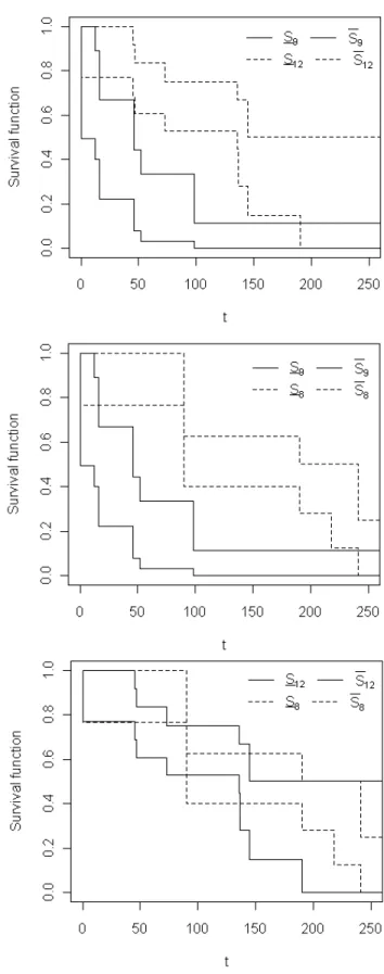
We can also compare these groups using the lower and upper survival functions, see Figure 1. In Figure 1, we provide the NPI lower and upper survival functions for case A1 where the first graph represents the lower and upper survival functions for the next units from groups I and II, the second graph represents the lower and upper survival functions for the next units from groups I and III and the third graph represents the lower and upper survival functions for the next units from groups II and III. Figure 1 shows indeed that the lifetime of a future unit from group I is likely to be less than the lifetime of a future unit from group II and III. However, we have weak evidence that the lifetime of a future unit from group II is less than the lifetime of a future unit from group III, and we see that the lower (and upper) survival functions for these groups cross each other.
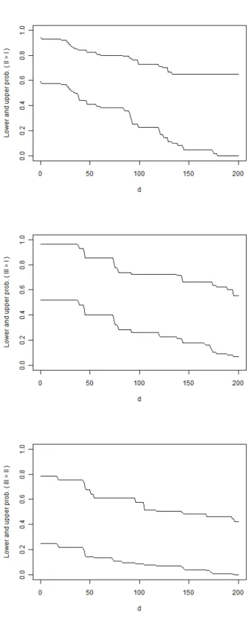
Figure 2 shows the NPI lower and upper probabilities for the events II>I, III>I and III>II for case A7 at different values of d, as presented in Section 6. These lower and upper probabilities are decreasing as functions of d, while the imprecision goes up and down reflecting the evidence in the data towards the events of interest. In fact, the imprecision is minimal at d = 0 for the event II>I, at 0 ≤ d ≤ 37 for the event III>I, and at d ≥ 196 for the event III>II. From the top plot in Figure 2 one can say that we have a strong indication that the lifetime of the next unit from group II is at least d greater than the lifetime of the next unit from group I for 0 ≤ d ≤ 34, as the lower probability P(II>I +d) ≥ 0.5 for these values of d. Similarly, from the middle plot in Figure 2 we have a strong indication that the lifetime of the next unit from group III is at least d greater than the lifetime of the next unit from group I for 0 ≤ d ≤ 38, as the lower probability P (III>I +d) ≥ 0.5 for these values of d. On the other hand, from the bottom plot in Figure 2 we have no evidence or indication that the lifetime of the next unit from group III is at least d greater than the lifetime of the next unit from group II for 0 ≤ d < 143, as P (III>II +d) ≤ 0.5 ≤ P (III>II +d) for these values of d. However, as P(III>II +d)< 0.5 for d≥ 143 we can say we have a strong indication for the complementary event, that the lifetime of the next unit from group III is not at least d greater than the lifetime of the next unit from group II, for d≥143, as P (III<II +d) = 1−P (III>II +d)≥0.5 for these values of d.
8. Concluding remarks
In this paper we presented NPI for pairwise comparison where each group is subject to several competing risks. We introduced NPI lower and upper probabilities for the event that the lifetime of the next unit from one group is greater than the lifetime of the next unit from the second group, taking into account these competing risks. We found that for fixed numbers of competing risks, e.g. after re-grouping competing risks into new defined competing risks, the lower and upper probabilities are the same regardless of how these competing risks are combined. We also found that studying the data in more detail, distinguishing more competing risks, leads to more imprecision.
Another interesting application of the work presented in this paper is the comparison of two sets of series systems lifetimes based on comparing the lifetimes of the two future series systems as we did in Sections 3, 4 and 5. We can do that as components within the series system are assumed independent and any failure of any of them will causes the system to fail, that is these components act as competing risks for the system (Kvam and Singh, 2001). By considering the NPI approach presented in Section 6, one can get a rich insight in the strength of the evidence in the data regarding the differences between these future series systems.
A special topic that involves right-censored data is progressive censoring (Balakrishnan and Aggarwala, 2000; Kundu et al., 2004), where, during a lifetime experiment, non-failing units are withdrawn from the experiments. This could be done to save cost or time, but it may also be useful, at the moment a unit fails, to study the unit in detail in comparison with units in the same experiment that have not failed, to get better knowledge about the underlying cause of failure. Maturi et al. (2010a) introduced NPI for comparing two groups of lifetime data under progressive censoring schemes, with careful discussion of different schemes and comparison to other frequentist approaches for such data. Later, Maturi et al. (2010b) considered progressive censoring combined with competing risks for inference on only one group, where further right-censored observations, due to the progressive censoring scheme, can be deal with in the same way as we dealt with the right-censored observations due to unknown failure modes or other unspecified reasons. Therefore, by applying that per group, i.e. X and Y, one can compare these two groups under progressive censoring with competing risks and use the NPI lower and upper probabilities introduced in Section 3.
Generalizing this NPI method for more than two groups is conceptually straightfor-ward but will lead to complications in notation, therefore developing R codes or other software is desirable, where R commands provided by Maturi (2010) could be a suitable starting point. For example, if interest is in selection of the best group, then one needs to calculate the lower and upper probabilities for the event that the next future observation from one group is greater than the next future observations from the other groups. If there is only one common failure mode which can cause the units to fail, then our results coincide with those obtained by Coolen-Maturi et al. (2012). Inclusion of assumed de-pendence between the competing risks in NPI framework would be an interesting topic for future research.
Appendices Appendix A
The NPI lower and upper probabilities (6) and (7) are derived as the sharpest bounds, based on the relevant rc-A(n) assumptions, for the probability
P =P(Xn+1< Ym+1) =P min 1≤j≤JXj,n+1 <1min≤l≤LYl,m+1 =P \ 1≤l≤L Yl,m+1 > min 1≤j≤JXj,n+1 ! = XXX C(j, ij) P \ 1≤l≤L ( Yl,m+1 > min 1≤j≤JXj,n+1 , \ 1≤j≤J Xj,n+1 ∈(xj,ij, xj,ij+1) )! where XXX C(j, ij)
denotes the sums over all ij from 0 to uj for j = 1, . . . , J.
To derive these NPI lower and upper probabilities, the lemma by Coolen and Yan (2003, p.153) is needed, using M-functions as defined in Section 2. First consider the lower probability (6), which is derived as the sharpest general lower bound for the above probability P, P ≥ XXX C(j, ij) P \ 1≤l≤L Yl,m+1 > min 1≤j≤J{xj,ij+1} ! J Y j=1 Pj(xj,ij, xj,ij+1) ≥ XXX C(j, ij) L Y l=1 υl X il=0 el,il X i∗l=0 1(gil
l,i∗l >1min≤j≤J{xj,ij+1})M l (gil l,i∗l, yl,il+1) J Y j=1 Pj(xj,ij, xj,ij+1)
The derivation of the corresponding NPI upper probability (7) is given below.
P ≤ XXX C(j, ij, i∗j) P \ 1≤l≤L Yl,m+1 > min 1≤j≤J{t ij j,i∗j} ! J Y j=1 Mj(tij j,i∗j, xj,ij+1) ≤ XXX C(j, ij, i∗j) " L Y l=1 υl X il=0
1(yl,il+1 > min 1≤j≤J{t ij j,i∗ j})P l(y l,il, yl,il+1) # J Y j=1 Mj(tij j,i∗ j, xj,ij+1) where XXX C(j, ij, i∗j)
denotes the sums over alli∗j from 0 tosj,ij and over all ij from 0 touj for
j = 1, . . . , J.
This results from the fact that for the lower (upper) probability, the first inequality follows by putting all probability mass for each Xj,n+1 (j = 1, . . . , J) assigned to the
intervals (tij
j,i∗j, xj,ij+1) (ij = 0, . . . , uj andi∗j = 0,1, . . . , sj,ij) at the right (left) end-points
of these intervals, and by using the lemma presented by Coolen and Yan (2003, p.153) for the nested intervals. The second inequality follows by putting all probability mass for Yl,m+1 (l = 1, . . . , L) in each of the intervals (gil,il∗l, yl,il+1) (il = 0, . . . , υl and i∗l =
Appendix B
In this appendix, the proof of (10) and (11) is given, where the following lemma (in-troduced and proven by Coolen-Maturi and Coolen (2011)) is needed.
Lemma: In case ofJ failure modes the following relation holds forXn+1 = min
1≤j≤J{Xj,n+1}, XXX C0(j, ij, xi+1= min 1≤j≤J{xj,ij+1}) J Y j=1 Pj(xj,ij, xj,ij+1) = S(xi) ˜ nxi+1+ 1 where XXX C0(j, ij, xi+1= min 1≤j≤J{xj,ij+1})
denotes the sums over all ij from 0 to uj for j = 1, . . . , J,
such that xi+1 = min
1≤j≤J{xj,ij+1}, where xi+1, i = 0, . . . , u −1, is the (i + 1)th failure
time (so ignoring the failure mode). Let xj,0 = 0 and x0 = min
1≤j≤J{xj,0} = 0, and
for i = u let xi+1 = xu+1 = ∞ and xu+1 = min
1≤j≤J{xj,uj+1} = min1≤j≤J{∞} = ∞, then Qs
j=1P
j(x
j,uj, xj,uj+1) = S(xu).
From the definition of the lower survival function (Coolen et al., 2002) and equation (5), the lower probability in (6) can be written as
P = u X i=0 X XX C(j, ij,xi+1= min 1≤j≤J{xj,ij+1}) L Y l=1 υl X il=0 el,il X i∗l=0 1(gil l,i∗l > xi+1)M l(gil l,i∗l, yl,il+1) J Y j=1 Pj(xj,ij, xj,ij+1) = u X i=0 X XX C(j, ij,xi+1= min 1≤j≤J{xj,ij+1}) L Y l=1 SY l,m+1(xi+1) J Y j=1 Pj(xj,ij, xj,ij+1) = u X i=0 SLCRYm+1(xi+1) XXX C(j, ij,xi+1= min 1≤j≤J{xj,ij+1}) J Y j=1 Pj(xj,ij, xj,ij+1) = u X i=0 SXn+1(xi) ˜ nxi+1+ 1 SLCRYm+1(xi+1)
The fourth equality above follows from the above lemma, where ˜nxu+1 = 0. Similarly, from the definition of the upper survival function (Coolen et al., 2002) and equation (5),
the upper probability in (7) can be written as P = n X i=0 XXX C(j, ij,i∗j,ti= min1≤j≤J{t ij j,i∗ j }) " L Y l=1 υl X il=0
1(yl,il+1 > ti)Pl(yl,il, yl,il+1)
# J Y j=1 Mj(tij j,i∗ j, xj,ij+1) = n X i=0 XXX C(j, ij,i∗j,ti= min 1≤j≤J{t ij j,i∗j}) L Y l=1 SYl,m+1(ti) J Y j=1 Mj(tij j,i∗j, xj,ij+1) = n X i=0 SYm+1(ti) X X X C(j, ij,i∗j,ti= min 1≤j≤J{t ij j,i∗j}) J Y j=1 Mj(tij j,i∗j, xj,ij+1) = n X i=0 SYm+1(ti) SJ CRXn+1(ti)−SJ CRXn+1(ti+1)
The fourth equality above follows from the definition of the NPI lower survival function (corresponding to failure modej) in terms ofM-functions as given in (Coolen et al., 2002) which is equivalent to equation (3).
References
Augustin, T., Coolen, F. P. A., 2004. Nonparametric predictive inference and interval probability. Journal of Statistical Planning and Inference 124 (2), 251–272.
Balakrishnan, N., Aggarwala, R., 2000. Progressive Censoring: Theory, Methods, and Applications. Birkha, Boston.
Bedford, T., Alkali, B., Burnham, R., 2008. Competing risks in reliability. In: Melnick, E. L., Everitt, B. S. (Eds.), Encyclopedia of Quantitative Risk Analysis and Assessment. Chichester: Wiley, pp. 307–312.
Borenstein, M., Hedges, L. V., Higgins, J. P. T., Rothstein, H. R., 2009. Introduction to Meta-Analysis. Wiley, Chichester.
Coolen, F. P. A., 2006. On nonparametric predictive inference and objective bayesianism. Journal of Logic, Language and Information 15 (1-2), 21–47.
Coolen, F. P. A., Augustin, T., 2009. A nonparametric predictive alternative to the im-precise dirichlet model: the case of a known number of categories. International Journal of Approximate Reasoning 50 (2), 217–230.
Coolen, F. P. A., Coolen-Schrijner, P., Yan, K. J., 2002. Nonparametric predictive infer-ence in reliability. Reliability Engineering & System Safety 78 (2), 185–193.
Coolen, F. P. A., Utkin, L. V., 2008. Imprecise reliability. In: Everitt, B. S., Melnick, E. L. (Eds.), Encyclopedia of Quantitative Risk Analysis and Assessment. Chichester:
Coolen, F. P. A., Yan, K. J., 2003. Nonparametric predictive comparison of two groups of lifetime data. In: Bernard, J. M., Seidenfeld, T., Zaffalon, M. (Eds.), ISIPTA’03: Proceedings of the Third International Symposium on Imprecise Probabilities and their Applications. pp. 148–161.
Coolen, F. P. A., Yan, K. J., 2004. Nonparametric predictive inference with right-censored data. Journal of Statistical Planning and Inference 126 (1), 25–54.
Coolen-Maturi, T., Coolen, F. P. A., 2011. Unobserved, re-defined, unknown or removed failure modes in competing risks. Journal of Risk and Reliability 225 (4), 461–474. Coolen-Maturi, T., Coolen-Schrijner, P., Coolen, F. P. A., 2011. Nonparametric
predic-tive selection with early experiment termination. Journal of Statistical Planning and Inference 141 (4), 1403–1421.
Coolen-Maturi, T., Coolen-Schrijner, P., Coolen, F. P. A., 2012. Nonparametric predic-tive multiple comparisons of lifetime data. Communications in Statistics - Theory and Methods 41 (22), 4164–4181.
De Finetti, B., 1974. Theory of Probability: A Critical Introductory Treatment. Wiley, London.
Hill, B. M., 1968. Posterior distribution of percentiles: Bayes’ theorem for sampling from a population. Journal of the American Statistical Association 63 (322), 677–691. Hill, B. M., 1988. De finetti’s theorem, induction, and an, or bayesian nonparametric
predictive inference (with discussion). In: Bernando, J. M., DeGroot, M. H., Lindley, D. V., Smith, A. (Eds.), Bayesian Statistics 3. Oxford University Press, pp. 211–241. Janurov´a, K., Briˇs, R., 2013. A nonparametric approach to medical survival data:
Un-certainty in the context of risk in mortality analysis. Reliability Engineering & System Safety.
URL http://www.sciencedirect.com/science/article/pii/S0951832013000902 Kalbfleisch, J. D., Prentice, R. L., 2002. The Statistical Analysis of Failure Time Data,
2nd Edition. John Wiley & Sons, NewYork.
Kaplan, E. L., Meier, P., 1958. Nonparametric estimation from incomplete observations. Journal of the American Statistical Association 53 (282), 457–481.
Kundu, D., Kannan, N., Balakrishnan, N., 2004. Analysis of progressively censored com-peting risks data. In: Balakrishnan, N., Rao, C. R. (Eds.), Handbook of Statistics 23: Advances in Survival Analysis. Amsterdam: Elsevier, pp. 331–348.
Kvam, P. H., Singh, H., 2001. On non-parametric estimation of the survival function with competing risks. Scandinavian Journal of Statistics 28 (4), 715724.
Luo, X., Turnbull, B. W., 1999. Comparing two treatments with multiple competing risks endpoints. Statistica Sinica 9 (4), 985–997.
Maturi, T., 2010. Nonparametric predictive inference for multiple comparisons. Ph.D. thesis, Durham University, Durham, UK, available from www.npi-statistics.com. Maturi, T. A., Coolen-Schrijner, P., Coolen, F. P. A., 2010a. Nonparametric predictive
comparison of lifetime data under progressive censoring. Journal of Statistical Planning and Inference 140 (2), 515–525.
Maturi, T. A., Coolen-Schrijner, P., Coolen, F. P. A., 2010b. Nonparametric predictive inference for competing risks. Journal of Risk and Reliability 224 (1), 11–26.
Park, C., Kulasekera, K. B., 2004. Parametric inference of incomplete data with competing risks among several groups. IEEE Transactions on Reliability 53 (1), 11–21.
Ray, M. R., 2008. Competing risks. In: Melnick, E. L., Everitt, B. S. (Eds.), Encyclopedia of Quantitative Risk Analysis and Assessment. Chichester: Wiley, pp. 301–307.
Sarhan, A. M., Hamilton, D. C., Smith, B., 2010. Statistical analysis of competing risks models. Reliability Engineering & System Safety 95 (9), 953 – 962.
Shafer, G., 1976. A Mathematical Theory of Evidence. Princeton University Press, Prince-ton (US).
Tsiatis, A., 1975. A nonidentifiability aspect of the problem of competing risks. In: Pro-ceedings of the National Academy of Sciences of the United States of America. 72. pp. 20–22.
Utkin, L. V., Coolen, F. P. A., 2007. Imprecise reliability: An introductory overview. In: Levitin, G. (Ed.), Computational Intelligence in Reliability Engineering, Volume 2: New Metaheuristics, Neural and Fuzzy Techniques in Reliability. New York: Springer, pp. 261–306.
Walley, P., 1991. Statistical Reasoning with Imprecise Probabilities. Chapman & Hall, London.
Weichselberger, K., 2000. The theory of interval-probability as a unifying concept for uncertainty. International Journal of Approximate Reasoning 24 (2-3), 149–170. Weichselberger, K., 2001. Elementare Grundbegriffe einer allgemeineren
Wahrschein-lichkeitsrechnung I. Intervallwahrscheinlichkeit als umfassendes Konzept. Physika, Hei-delberg.