IMPROVED LEARNING OF STRUCTURAL
SUPPORT VECTOR MACHINES: TRAINING
WITH LATENT VARIABLES AND NONLINEAR
KERNELS
A Dissertation
Presented to the Faculty of the Graduate School of Cornell University
in Partial Fulfillment of the Requirements for the Degree of Doctor of Philosophy
by Chun Nam Yu
c
2011 Chun Nam Yu ALL RIGHTS RESERVED
IMPROVED LEARNING OF STRUCTURAL SUPPORT VECTOR MACHINES: TRAINING WITH LATENT VARIABLES AND NONLINEAR KERNELS
Chun Nam Yu, Ph.D. Cornell University 2011
Structured output prediction in machine learning is the study of learning to predict complex objects consisting of many correlated parts, such as sequences, trees, or matchings. The Structural Support Vector Machine (Structural SVM) algorithm is a discriminative method for structured output learning that allows flexible feature construction with robust control for overfitting. It provides state-of-art prediction accuracies for many structured output prediction tasks in nat-ural language processing, computational biology, and information retrieval.
This thesis explores improving the learning of structured prediction rules with structural SVMs in two main areas: incorporating latent variables to ex-tend their scope of application and speeding up the training of structural SVMs with nonlinear kernels. In particular, we propose a new formulation of struc-tural SVM, called Latent Strucstruc-tural SVM, that allows the use of latent variables, and an algorithm to solve the associated non-convex optimization problem. We demonstrate the generality of our new algorithm through several structured output prediction problems, showing improved prediction accuracies with new alternative problem formulations using latent variables.
In addition to latent variables, the use of nonlinear kernels in structural SVMs can also improve their expressiveness and prediction accuracies. How-ever their high computational costs during training limit their wider applica-tion. We explore the use of approximate cutting plane models to speed up
the training of structural SVMs with nonlinear kernels. We provide a theoret-ical analysis of their iteration complexity and their approximation quality. Ex-perimental results show improved accuracy-sparsity tradeoff when compared against several state-of-art approximate algorithm for training kernel SVMs, with our algorithm having the advantage that it is readily applicable to struc-tured output prediction problems.
BIOGRAPHICAL SKETCH
Chun-Nam Yu was born and grew up in Hong Kong, spending the first two decades of his life there. In 2001 he travelled to England to pursue university education, that being the very first time he stepped outside Asia. After over-coming the weather and the food he began to appreciate and enjoy studying inside the historic buildings at Oxford, and loved the weekly academic discus-sions with his tutors in Wadham College. He earned a BA degree in Mathemat-ics and Computer Science with First Class Honours in 2004, and then moved across the Atlantic to pursue a PhD degree in Computer Science at Cornell Un-versity. There he saw real snow for the first time and studied under the guid-ance of Professor Thorsten Joachims. He learned to do research in machine learning, working mainly in the area of support vector machines and structured output learning. After finishing his PhD he continues his trajectory towards the northwest to brave colder weather and will become a postdoctoral fellow at the Alberta Ingenuity Center for Machine Learning at the University of Alberta in Canada.
ACKNOWLEDGEMENTS
First of all I must thank my PhD advisor Professor Thorsten Joachims, for his mentorship and friendship over these years. Looking back, his wise and patient guidance over these six years transformed me from an inexperienced under-graduate to an independent researcher ready to tackle problems on his own. It is hard to describe either my gratitude or my good luck in having Thorsten as my advisor. His taste and choice of problems, discipline and commitment to hard work, all had a great influence on me. His patience during my ups and downs, his encouragement to me to try new and bolder approaches and prob-lems, all made my PhD journey much smoother and at the same time much more exciting.
I would also like to thank my committee members, Professor Adam Siepel and Professor Mike Todd. Their careful reading of this thesis helps improve its presentation greatly. I want to thank Adam for teaching me graphical models and many things in computational biology, and Mike for teaching me optimiza-tion and for his discussions when I encountered issues involving optimizaoptimiza-tion in my research. Many other mentors also helped me greatly in my development during these PhD years, to whom I want to express my gratitude: to Professor Ron Elber for his encouragement and collaboration for my first research project at Cornell; to Dr Balaji Krishnapuram at Siemens for teaching me good work habits and time management in my first summer internship; and to Dr Sathiya Keerthi at Yahoo! Research for his interest in my development and discussions of research problems.
To my fellow PhD students I need to thank Dan Sheldon, Tudor Marian, and Kevin Walsh for being great officemates for many years. Thanks must also be given to fellow students in the Machine Learning Discussion Group
(MLDG) over the years for their friendships and collaboration, including Alex, Niculescu-Mizil, Filip Radlinski, Tom Finley, Benyah Shaparenko, Art Munson, Yisong Yue, Daria Sorokina, Nikos Karampatziakis and Ainur Yessenalina. Pa-per discussions and brainstorming half-baked ideas with them made studying and doing research in machine learning a much more fun experience.
I would also like to thank all the brothers and sisters in the Hong Kong Christian Fellowship and FICCC over the years for all their encouragements and prayers. Their love makes the winter in Ithaca warm. And thank God for His faithfulness and answering of my prayers, for the blessings I’ve received during these six years in Ithaca far exceed what I have asked or imagined.
Finally I need to thank my parents, my brother and my sister for their en-during patience and support over all these years when I am away from home, and for their believes in me in completing this degree. This thesis is dedicated to them.
The works presented in this thesis are supported by the grants NSF-Project IIS-0713483, NSF-Project IIS-0412894, and NSF-Project IIS-0905467.
TABLE OF CONTENTS
Biographical Sketch . . . iii
Dedication . . . iv
Acknowledgements . . . v
Table of Contents . . . vii
List of Tables . . . x
List of Figures . . . xi
1 Introduction 1 1.1 Structured Output Prediction . . . 1
1.2 Generative and Discriminative Models . . . 4
1.2.1 Generative Models for Structured Output Predictions . . . 5
1.2.2 Discriminative Models for Structured Output Predictions 7 1.3 Structural Support Vector Machines . . . 10
1.4 Organization and Contributions of this Thesis . . . 12
1.4.1 Structural SVM for Protein Alignments . . . 12
1.4.2 Latent Structural SVM . . . 13
1.4.3 Training Nonlinear Structural SVMs with Kernels using Approximate Cutting Plane Models . . . 14
1.4.4 Thesis Organization . . . 15
2 Structural Support Vector Machines 17 2.1 A Part-Of-Speech Tagging Example . . . 17
2.2 Support Vector Machines . . . 22
2.3 From Binary to Multi-Class Support Vector Machines . . . 29
2.4 From Multi-class to Structural Support Vector Machines . . . 31
2.4.1 Kernels in Structural SVMs . . . 35
2.4.2 Slack-rescaling . . . 36
2.5 Bibliographical Notes . . . 38
2.5.1 Related Models . . . 38
2.5.2 Applications of Structural SVMs . . . 42
3 Cutting Plane Algorithms for Training Structural SVMs 44 3.1 Cutting Plane Algorithm . . . 45
3.2 Proof of Iteration Bound . . . 51
3.3 Loss-Augmented Inference . . . 56
3.4 Bibliographical Notes . . . 58
4 Structural SVMs for Protein Sequence Alignments 60 4.1 The Protein Sequence Alignment Problem . . . 60
4.2 Sequence Alignments and the Inverse Alignment Problem . . . . 63
4.2.1 Dynamic Programming for Sequence Alignments . . . 64
4.3 Learning to Align with Structural SVMs . . . 69
4.3.1 Loss Functions . . . 70
4.4 Aligning with Many Features . . . 73
4.4.1 Substitution Cost Model . . . 74
4.4.2 Gap Cost Model . . . 78
4.5 Experiments . . . 79
4.5.1 Data . . . 79
4.5.2 Results . . . 81
4.6 Conclusions . . . 86
4.7 Bibilographical Notes . . . 87
5 Structural SVMs with Latent Variables 88 5.1 Latent Information in Structured Output Learning . . . 88
5.2 Structural SVMs with Latent Variables . . . 90
5.3 Training Algorithm . . . 95
5.4 Three Example Applications . . . 98
5.4.1 Discriminative Motif Finding . . . 98
5.4.2 Noun Phrase Coreference Resolution . . . 100
5.4.3 Optimizing Precision@kin Ranking . . . 104
5.5 Conclusions . . . 107
5.6 Bibliographical Notes . . . 108
6 Training Structural SVMs with Nonlinear Kernels 110 6.1 Nonlinear Support Vector Machines with Kernels . . . 110
6.2 Kernels in Structural SVMs . . . 114
6.3 Cutting Plane Algorithm for Kernel SVMs . . . 115
6.4 Cut Approximation via Sampling . . . 119
6.4.1 Convergence and Approximation Bounds . . . 121
6.4.2 Experiments . . . 128
6.5 Cut Approximation via Preimage Optimization . . . 135
6.5.1 The Basis . . . 137
6.5.2 Projection . . . 138
6.5.3 Basis Extension . . . 139
6.5.4 Theoretical Analysis . . . 140
6.5.5 Experiments . . . 143
6.6 Applications in General Structural SVMs . . . 149
6.7 Conclusions . . . 150
6.8 Bibliographical Notes . . . 151
7 Conclusions and Future Directions 153 7.1 Conclusions . . . 153
7.2 Future Directions . . . 156
7.2.1 Approximate Inference for Training . . . 156
7.2.3 Reducing Dependence on Labeled Data . . . 158
LIST OF TABLES
2.1 Conditional Probabilty Tables for HMM example . . . 19
4.1 Q-score of the SVM algorithm for different alignment models (average of 5CV, standard error in brackets). . . 82
4.2 Comparing training for Q-score with training forQ4-score by test set performance. . . 83
4.3 Comparing training for Q-score with training for Q4-score by test set performance. . . 85
5.1 Classification Error on Yeast DNA (10-fold CV) . . . 100
5.2 Clustering Accuracy on MUC6 Data . . . 103
5.3 Precision@kon OHSUMED dataset (5-fold CV) . . . 107
6.1 Runtime and training/test error of sampling algorithms com-pared to SVMlightand Cholesky. . . 134
6.2 Prediction accuracy with kmax = 1000 basis vectors (except SVMlight, where the number of SVs is shown in the third line) using the RBF kernel (except linear). . . 145
6.3 Number of SVs to reach an accuracy that is not more than 0.5% below the accuracy of the exact solution of SVMlight(see Ta-ble 6.2). The RBF kernel is used for all methods. ’>’ indicates that the largest tractable solution did not achieve the target accu-racy. . . 148
6.4 Training time to reach an accuracy that is not more than 0.5% be-low the accuracy of the exact solution of SVMlight(see Table 6.2). The RBF kernel is used for all methods. ’>’ indicates that the largest tractable solution did not achieve the target accuracy. . . 149
LIST OF FIGURES
1.1 Three examples of structured output prediction problems . . . . 2
1.2 Examples of generative structures: HMM for speech recognition example (left) and parse tree (right) . . . 5
2.1 HMM example . . . 18
2.2 Binary Support Vector Machines . . . 24
2.3 Binary Support Vector Machine with Slack Variables . . . 25
2.4 Binary support vector Machine with slack variables, with sup-port vectors highlighted . . . 27
2.5 Binary SVM with Gaussian Kernels. The solid line is the decision boundary, while the dotted lines arew·x=±1. Notice the ability to introduce nonlinear and even disjoint decision regions using the Gaussian kernel. . . 28
2.6 Illustration of the joint feature mapΦapplied to the HMM example 33 2.7 Structural Support Vector Machine on POS tagging example . . . 34
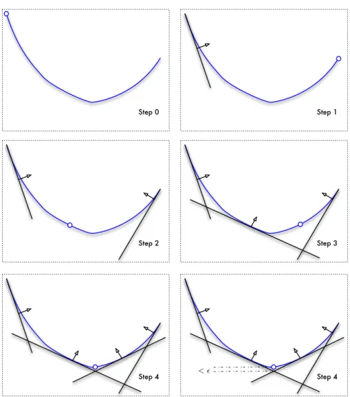
3.1 Illustration of cutting plane algorithm: the blue curve is the true objective function, while the black straight lines are the cutting planes. . . 48
4.1 The 20 Common Amino Acids . . . 62
4.2 BLOSUM62 substitution matrix . . . 65
4.3 Dynamic Programming Table for Sequence Alignments . . . 67
4.4 Illustration of Q-loss: out of three ”match” operations in the reference alignment, the alternative alignment agrees on two of them. The Q-loss is therefore1/3. . . 71
4.5 Illustration of Q4-loss: out of three ”match” operations in the reference alignment, the alternative alignment has all three of them aligned to another residue within shift 4. The Q4-loss is therefore0. . . 71
4.6 Q-score of theAnova2alignment model againstC. . . 83
5.1 French-English word alignment example from Brown et al. [17] . 89 5.2 The circles are the clusters defined by the labely. The set of solid edges is one spanning foresththat is consistent withy. The dot-ted edges are examples of incorrect links that will be penalized by the loss function. . . 101
5.3 Latent Structural SVM tries to optimize for accuracy near the region for the top k documents (circled), when a good general ranking directionwis given . . . 106
6.1 Proof Idea for Theorem 6.2: the objective difference betweenw∗ and v∗ is bounded by + γ. is the usual stopping criterion whileγis the error introduced by the use of approximate cutting planes, and is bounded by
q
4CR2 k log
T
δ. . . 128
6.2 CPU Time Against Training Set Size . . . 130
6.3 Training Set Error Against Training Set Size . . . 130
6.4 Test Set Error Against Training Set Size . . . 131
6.5 CPU Time(Left) and Number of Iteration (Right) Against Sample Size . . . 132
6.6 Training Set Error(Left) and Test Set Error(Right) Against Sample Size . . . 132
6.7 Decrease in accuracy w.r.t. exact SVM for different basis-set sizes kmax. . . 146
CHAPTER 1 INTRODUCTION
1.1
Structured Output Prediction
Structured output prediction is the problem of teaching machines to predict complex structured output objects such as sequences, trees, or graph matchings. It includes a very broad and diverse set of tasks, for example, parsing a Chinese sentence, aligning two protein sequences, segmenting a picture into people and objects, or translating a Japanese news article into English. It is very different from traditional tasks in machine learning and statistics such as classification or regression, where the output setY contains only simple categorical labels or real values.
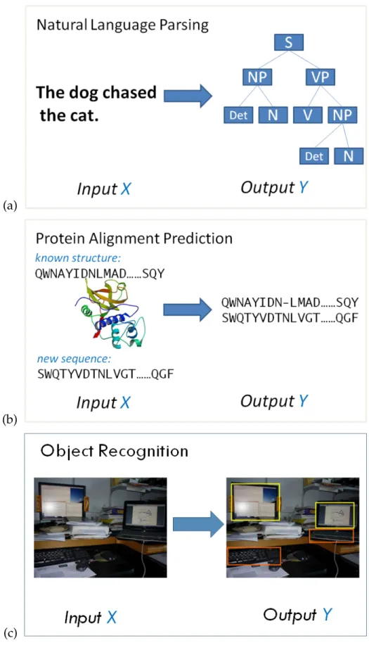
Figure 1.1 shows three specific structured output prediction tasks: parsing, protein sequence alignment, and object recognition. In natural language pars-ing (Figure 1.1(a)), the input spaceX is the set of well-formed English sentences, and the output space Y is the set of parse trees that show how the words are joined together to form meaningful sentences. In protein sequence alignment (Figure 1.1(b)), the input spaceX contains protein sequence pairs from a pro-tein database, and the output space Y consists of alignments between these sequence-pairs that align structurally similar regions together. In object recog-nition (Figure 1.1(c)), the input space X can be different images taken inside offices, and the output space Y is the set of bounding boxes around monitors and keyboards inside the image.
(a)
(b)
(c)
traditional machine learning problems such as classification or regression? The first observation is that these complex output objects usually consist of many correlated ”parts”. In Figure 1.1, the terminal node labels in the parse tree de-pends on the node labels of their parents. For example a verb phrase (VP) has to contain a verb (V) in its children. The alignment operations in protein sequence alignments also depend on the neighbouring alignment operations. For exam-ple, it is much more common to have long stretches of aligned amino acids or long stretches of unaligned gaps than to have short interleaving of aligned and unaligned positions. The neighbouring pixels in an image tend to belong to the same object, and different object-pairs can have certain spatial relations (e.g., it is quite common to locate a monitor above a keyboard). These local and global dependencies between the ”parts” have to be taken into account when mak-ing predictions. These statistical dependencies are quite commonly, though not always necessarily, expressed using graphical models [70].
Another prominent common feature of these structured prediction tasks is the use of combinatorial optimization and search algorithms in prediction. For example, parsing can be performed using the CYK algorithm [72, 149], protein sequence alignments can be computed using the Smith-Waterman algorithm [118], which are both dynamic programming based algorithms. Image segmen-tation can be computed using graph cuts [16]. Once the local and global de-pendencies between the ”parts” are fixed and the cost parameters determined, these combinatorial optimization algorithms help us to find out the highest scor-ing output parse tree, alignment, or segmentation. The problem of structured output learning is to learn the cost parameters so that the parse trees, align-ments, or segmentations are as close to what we observe in the training set as possible. Thus it can be regarded in some way as the inverse problem of
combi-natorial optimization. We try to find out parameters given example structures, as opposed to finding highest scoring structures given fixed parameters.
1.2
Generative and Discriminative Models
We can state the structured output prediction problem more formally as follows. Given a set of training examplesS ={(x1, y1), . . . ,(xn, yn)} ∈(X ×Y)n, we want
to learn a prediction functionh:X → Y in the following form:
h(x) = argmaxy∈Yfθ(x, y). (1.1)
The functionf is a scoring function that evaluates how well a particular output structurey ∈ Y matches an input x ∈ X, and it is parameterized by the vector θ that we want to learn. The argmax over all possibley ∈ Y extracts the high-est scoring output as the prediction for x, and is usually computed using the combinatorial optimization algorithms such as the CYK algorithm or the Smith-Waterman algorithm previously mentioned. This is a very general setting that includes most learning problems for structured output prediction.
How should we learn the parameter vector θ so that predictions that are close to what we observe in the training set can be reproduced? There are cur-rently two main approaches for this. The first approach is called generative modeling while the second approach is called discriminative modeling.
Ithaca is gorgeous "Ithaca" "is" "gorgeous" S NP VP Det N V NP Det N
The dog chased
the cat
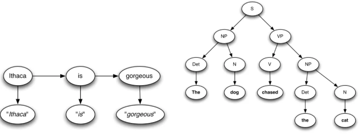
Figure 1.2: Examples of generative structures: HMM for speech recogni-tion example (left) and parse tree (right)
1.2.1
Generative Models for Structured Output Predictions
Given an inputxand an outputy, generative model tries to estimate a joint dis-tributionP(x, y)ofxandy. However this is usually a difficult problem to tackle directly given that bothxandyare complex high-dimensional objects. The key idea here is to break down the complexity or high dimensionality by explicitly stating how the complex input-output pair(x, y) are generated by composing simple parts, and thus the namegenerativemodeling. This is also equivalent to stating how the complex distributionP(x, y)factorizes into a product of simpler distributions on the parts inx, y.
The classic Hidden Markov Model (HMM) [105] is a good example of gener-ative modeling, and it was very widely applied to the problem of speech recog-nition in the early days. In speech recogrecog-nition (a simplified version of the prob-lem) the inputx(called observations) is a sequence of sounds in human speech, and the output y (called hidden states) is a corresponding set of words in the English language. Hidden Markov models make the assumption that the ob-servations at time stept are generated by the hidden state at time step t only,
and the hidden state at time stept depends only on the previous hidden state at time step t−1. Thus to generate English speech for the sentence ”Ithaca is gorgeous”, we would first generate the word ”Ithaca” randomly from the initial distribution, and then generate a pronunciation of ”Ithaca” from our emission distribution. Next we generate a second English word conditioned on the pre-vious word ”Ithaca”, and suppose the word is ”is”, and after that we generate a pronunciation of ”is” using the emission distribution. And we repeat the same for the third word ”gorgeous”. Thus the process of generating human speech can be modeled in a very simple linear fashion (Figure 1.2, left).
As another example let us look at the parse tree of the sentence ”The dog chased the cat” in Figure 1.2. We can imagine there is a stochastic process (stochastic context free grammar) that starts from the root of the tree as a whole sentence (S), and then split into a pair of noun phrase (NP) and verb phrase (VP). The noun phrase then splits into a determiner (”the”) and a noun (”dog”), and the verb phrase further splits into a verb and a noun phrase that gives the whole subtree for the expression ”chases the cat”. At each node we generate a leaf node or an internal node conditioned on the previous splits in the tree according to a local conditional probability distribution. For different runs we could have gen-erated alternative sentences and parse trees such as ”The cat chased the dog”, or ”The dog chased the fat cat” in these tree growing processes.
For both the HMM and parse tree generation example the observed input-output pair (x, y) are generated sequentially, part by part, through simple stochastic generative processes. These processes are completely specified by local conditional probability tables that govern the decision at each step. To put it more precisely, we estimate our scoring functionf by taking it to be the joint
probability (or equivalently its logarithm): fθ(x, y) =Pθ(x, y) = Y i P(yi |π(yi)) Y j P(xj |π(xj)),
wherexj,yiare the observed and hidden nodes in the directed acyclic graphs in
Figure 1.2. The notationπ(u)refers to the parent node ofuin the directed acyclic graph. The local conditional probabilities for transitions between hidden nodes
P(yi | π(yi))and emissions for observed nodesP(xj |π(xj))are the parameters
in the vectorθ.
Since the complex process of jointly generating a speech sequence and an English sentence (or a parse tree and an English sentence in the other example) is broken down into a series of local decisions, parameter estimation ofθthrough maximum likelihood becomes easy as in most cases it boils down to counting.
1.2.2
Discriminative Models for Structured Output Predictions
The second approach is called discriminative modeling, which takes a com-pletely different view on structured output prediction. The training sample we are given comes in the form of input-output pairs(x, y) ∈ X × Y. Generative modeling tries to model all the observations by estimating a joint distribution
P(x, y). However if we think carefully this is not exactly the task that we are given. Consider a hypothetical extreme case when there is one possible output
y0 ∈ Y, then no matter what the inputxis all we can do is to predicty0. It will be a huge waste of effort to model the joint distributionP(x, y)(which is essentially
P(x)) in this case, since the inputxcan have arbitrarily complex distribution but it would not help us in the prediction of y at all. Even not in this extreme
sit-uation it is quite common to have information in input xthat is irrelevant for the prediction ofy. For example, when we are building a generative model for detecting whether there are humans in a picture, we could be spending a lot of effort to model all the clutter and non-human objects in the background in order to estimate a good joint distributionP(x, y).
A second major difficulty in applying generative models in practice is that they are difficult to design. While generative models for the sequence tagging and parse tree examples are relatively straightforward and reasonable, in many structured output prediction problems it is very hard to design a generative model that explains all the observed features in input x well. In the human-detection example just mentioned it is almost impossible to describe a good generative process that models all the clutter and background objects on pic-tures with humans on it. In machine translation it is also difficult to describe a generative model that transforms a French sentence into an English sentence. Many simplifying assumptions have to be made [17], such as each word being translated independently or the limited re-arrangement when translating from French into English. In the protein alignment example that we are going to discuss in Chapter 4, it is not easy to decide whether to assume (which is obvi-ously wrong biologically) that the amino acid identity at an aligned position is independent of their secondary structures to simplify the parameter estimation. These modeling decisions are really hard to make and worse still we might have to re-design the model structures whenever we obtain new observed features.
Discriminative modeling tries to sidestep all these problems in generative modeling by tackling the estimation of the scoring functionf in Equation (1.1) directly. It tries to learn a function f such that good output structures score
higher than bad output structures for a fixed input x, and hence the name dis-criminative modeling, because the functionf helps us to differentiate between good and bad output structures. No attempt is made on modeling the input distribution forxor the joint distributionP(x, y), and thus a lot of the difficult modeling decisions can be avoided. One common choice is to assumef to be linear, with
fθ(x, y) = θ·Φ(x, y),
whereΦ(x, y)is a high dimensional feature vector that extracts features which indicate whether the input-output pair(x, y)is a good fit or not.
Conditional random field (CRF) [81], a discriminative structured output learning method, finds the parameter vector θ and hencef by minimizing the following objective: min θ 1 2kθk 2 −C n X i=1 [θ·Φ(xi, yi)−log X ˆ y∈Y exp(θ·Φ(xi,yˆ)) ! ]. (1.2)
Structural support vector machine (Structural SVM) [132], which is the topic of this thesis, findsf by minimizing the following objective:
min θ 1 2kθk 2 +C n X i=1 max ˆ y∈Y[θ·Φ(xi,yˆ)−θ·Φ(xi, yi) + ∆(yi,yˆ)], (1.3)
where∆is a loss function measuring how different the outputyˆis when com-pared against the reference outputyi.
We shall have a more in-depth discussion of these methods in the next chap-ter. Ignoring the regularization term1/2kθk2 for the moment, we can see that both CRFs and structural SVMs try to set the score of the correct output yi in
the training set higher than alternative outputsyˆ∈ Y, though through different ways. CRFs acheive this by maximizing the conditonal likelihoodP(y |x), try-ing to make the score of the correct outputθ·Φ(xi, yi)large with respect to the
log-sum of all other outputslog(Pyˆ∈Yexp(θ·Φ(xi,yˆ))). Structural SVMs achieve
this by maximizing the score difference between the correct outputθ·Φ(xi, yi)
and the scores of all other outputsθ·Φ(xi,yˆ), with the required margin enforced
by a loss function∆.
We can see in both of these objectives efforts are made to discriminate the correct outputyiagainst all alternative outputsyˆthat are not observed, while no
effort is made to model the input distribution forxi (or any alternative inputs).
As far as the minimization objective is concerned all the inputsxiare fixed. This
is a common feature of discriminative modeling, and can be seen as a more pragmatic approach compared to the more ambitious approach of joint density estimation in generative modeling.
1.3
Structural Support Vector Machines
Structural support vector machine (Structural SVM), the focus of this thesis, is a very successful and popular algorithm for discriminative structured output learning. First as a discriminative learning algorithm it allows flexible con-struction of features to improve prediction accuracy. As in Equation (1.3) the distribution of inputxi is not explicitly modeled, allowing us to construct
com-plex features based on the input xi in the joint feature vector Φ(x, y) without
modifying the structure of the optimization problem. This particular flexibil-ity and ease to incorporate new features to improve prediction performance are the main reasons for the popularity of discriminative models such as structural SVMs and CRFs in recent years.
con-struct rich features from the input x to improve prediction accuracy, it also becomes much easier to overfit to the training data when we have the power to incorporate these high dimensional input features. Structural SVM, like the binary support vector machine for classification, controls overfitting by maxi-mizing the margin between alternative outputs. The influential work of Vapnik [133] on regularized risk minimization laid the foundation for discriminative modeling, where the importance of capacity control (regularization) is empha-sized and linked to the generalization ability of learning algorithms. Regular-ization is particularly important when we have high dimensional feature space and small training sample sizes. The implementation of this idea in the form of Support Vector Machines (SVM) gives rise to one of the most popular machine learning algorithm in the last decade [34], with high classification accuracies on many applications such as text classification [62], object recognition [103], classification of gene expression data [56], and countless many other applica-tions. Binary SVMs work by constructing a large-margin hyperplane in high dimensional feature space as a separator between positive and negative exam-ples. Structural SVM is a generalization of binary SVMs for structured output learning. It inherits many of the attractive properties of SVMs, such as the abil-ity to explicitly control margins between different outputs, the abilabil-ity to incor-porate high dimensional input features without overfitting, and the ability to incorporate nonlinear kernels.
Thirdly compared to CRFs, structural SVMs do not require the computation of log-sum over all possible output structures (called the partition function) in Equation (1.2). This can be beneficial in certain cases such as learning match-ings or spanning trees, when computing the sum over all possible matchmatch-ings or spanning trees have a higher computational complexity than computing the
highest scoring output structure. The explicit use of a loss function ∆ to con-trol the margins also helps us tune the parameter vector in different application settings. Because of all these advantages structural SVMs have been applied to many different applications in diverse domains, including natural language processing, computational biology, information retrieval, computer vision, etc. We will discuss some of these applications in greater detail in the later chapters.
1.4
Organization and Contributions of this Thesis
This thesis presents some new results on discriminative structured output learn-ing based on structural SVMs.
1.4.1
Structural SVM for Protein Alignments
Protein sequence alignment is an important step in the homology modeling ap-proach for solving protein structures, but it is also a very hard problem for se-quence pairs with low sese-quence similarity but high structural similarity. There are a lot of relevant information for determining the alignment such as amino acid residue, secondary structures, water accessibility, and evolutionary infor-mation through PSI-BLAST profiles in databases for proteins with known struc-tures. This is an ideal application for discriminative structured output learning since we can incorporate all these rich features without having to model their dependencies. In this thesis we apply the structural SVM algorithm to learn protein alignment models incorporating these rich features over a large dataset. Experiments show that it outperforms some of the state-of-art generative
align-ment models on large test sets and is practical to train. This application also illustrates many of the design decisions in applying structural SVM for struc-tured output learning such as the design of feature maps and loss functions, and also choosing a corresponding efficient inference procedure for training.
1.4.2
Latent Structural SVM
Despite the success of structural SVMs in many different applications, there are still issues that hinder their even wider adoption. One important issue is their inability to handle latent variables or missing information. In many applications in natural language processing and computer vision some of the crucial mod-eling information is not present in the training data, and yet it is important to include it to learn models of good predictive performance. For example in ob-ject or human recognition, it is important to know the positions of the parts of an object to accurately recognize the object, such as the positions of the wheels in a car or the positions of arms and legs of a pedestrian. And yet as labels we are only given a rough bounding box on where the target object is without any information on the parts. As another example consider the training data we usually have in machine translation, which are sentence-pairs in the source language (say French) and the target langauge (say English). However, it will be really useful to know roughly which French word corresponds to which En-glish word in the sentence pair, but such information is usually not available. In this thesis we give the first natural extension of the structural SVM algo-rithm to handle latent variables. This greatly increases the scope of application of the structural SVM algorithm to new problems, and also allows us to solve old problems in new formulations. We give efficient training algorithm for our
latent structural SVM formulation, and demonstrate how it can be applied via three different applications in computational biology, natural language process-ing, and information retrieval.
1.4.3
Training Nonlinear Structural SVMs with Kernels using
Approximate Cutting Plane Models
The ability to produce nonlinear decision boundaries through the use of kernels was one of the main reasons of the wide applicability and popularity of support vector machines in classification. Using kernels such as the polynomial kernels and the Gaussian kernel, SVM is one of the best off-the-shelf classification algo-rithms when applied to a new classification problem without any tuning. The use of nonlinear kernels in structured output learning is equally beneficial since it allows the learned function for scoring different output structures to become nonlinear. However, the cost of training nonlinear SVMs with kernels is much higher than training linear SVMs because the target function we learn is rep-resented implicitly as a sum of kernel functions evaluated at a large number of training points. There are many works on approximation in training binary classification SVMs with kernels [145, 46, 131, 14], but they are either not di-rectly applicable to structural SVMs without significant modification or they do not give good enough tradeoffs between approximation quality and training costs. In this thesis we propose to directly modify the cutting plane algorithm for the approximation. The cutting plane algorithm is one of the most suc-cessful algorithm for training support vector machines and structural support vector machines. We will explore approximating each cutting plane generated
by the cutting plane algorithm so that the cost of kernel function evaluations is reduced. In particular we are going to look at two different approximation schemes, one using random sampling and the other using a preimage optimiza-tion approach. Our proposed algorithms result in improved training time by reducing the number of kernel evaluations required while maintaining accu-racies close to the exact algorithm, and the preimage approach also has better accuracy-sparsity tradeoff when compared against other approximation algo-rithms on binary classification. Moreover they can be easily extended to handle the use of nonlinear feature functions in structural SVMs.
1.4.4
Thesis Organization
This thesis is organized as follows. In Chapter 2 we give an introduction to dis-criminative training of structured output prediction models, with an emphasis on structural SVMs.
In Chapter 3 we describe in detail the cutting plane algorithm for solving the optimization problems associated with structural SVMs. It provides the basis for the various algorithms discussed in the following chapters.
In Chapter 4 we illustrate the benefits and challenges of discriminative train-ing through our work on ustrain-ing structural SVMs to train alignment models for protein sequence alignments.
In Chapter 5 we describe our work on extending structural SVMs to handle latent variables, which greatly extends their scope of applications.
structural SVMs with approximate cutting plane models, specifically for the cases where nonlinear kernels are used.
Chapter 7 contains our concluding remarks and points out some interesting future research directions.
CHAPTER 2
STRUCTURAL SUPPORT VECTOR MACHINES
2.1
A Part-Of-Speech Tagging Example
In this chapter we are going to introduce Structural Support Vector Machines (Structural SVMs) and see how we can use it for predicting structured outputs. For this purpose let us use a very simple example to see how we can do struc-tured output prediction with traditional generative modeling, and then see how it can be modeled discriminatively with structural SVMs. The example appli-cation that we are going to consider is part-of-speech tagging (POS tagging) in natural language processing.
Given an English sentence, part-of-speech tagging tries to determine each word in the sentence to see whether it is a noun, a verb, an adjective, a deter-miner, etc. It is not a trivial task as many English words can have more than one part-of-speech (e.g., ”bank” as verb and ”bank” as noun). It is a very basic low-level task in natural language processing that supports many other higher low-level tasks such as question-answering, sentiment analysis, etc. For example, know-ing where the nouns are can help us recognize what people or organizations are involved, knowing the verb can help us understand what is happening, and knowing the adjective can help us decide the speaker’s opinion or sentiment. It is a structured-output prediction task as the part-of-speech tag at each position in the sentence is highly correlated with the POS tags at the positions immedi-ately before and after it.
noun verb noun noun noun
I like support vector machines
x1 x2 x3 x4 x5 y5 y4 y3 y2 y1 BEGIN END Figure 2.1: HMM example
data is Hidden Markov Model (HMM) [105]. Hidden Markov models estimates the joint distribtionP(x, y)between the inputx= (x1, x2, . . . , xL)(called the
ob-servation sequence) and the outputy = (y1, y2, . . . , yL)(called the hidden state
sequence), where L is the length of the sequence. It tells us how an (x, y) se-quence pair can be generated one position after another by making stochastic local decisions. Consider the sentence ”I like support vector machines” in Fig-ure 2.1, with the correct part-of-speech tags ”Noun Verb Noun Noun Noun”. The outputsyiare the part-of-speech tags, and they are also called hidden states
in HMM terminology as they are not observed and are the labels that we want to predict. The inputsxi are the English words, and they are called the
obser-vations. The arrows in the figure indicate dependency relations, and we can see that each hidden stateyi only depends on the immediate hidden stateyi−1 before it. This is the Markov assumption and hence the name hidden Markov models. Also, each observation xi also only depends on the hidden state yi at
the same position.
Thus we can generate the whole (x, y) pair by making sequential local de-cisions. We can generate the first hidden statey1 by throwing a dice according
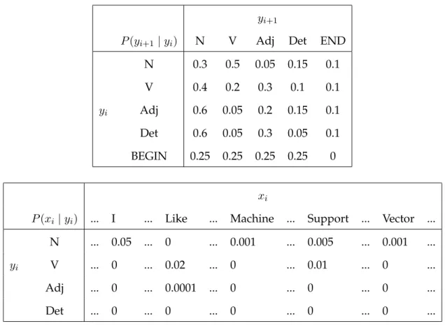
Table 2.1: Conditional Probabilty Tables for HMM example
yi+1
P(yi+1 |yi) N V Adj Det END
N 0.3 0.5 0.05 0.15 0.1 V 0.4 0.2 0.3 0.1 0.1 yi Adj 0.6 0.05 0.2 0.15 0.1 Det 0.6 0.05 0.3 0.05 0.1 BEGIN 0.25 0.25 0.25 0.25 0 xi
P(xi |yi) ... I ... Like ... Machine ... Support ... Vector ... N ... 0.05 ... 0 ... 0.001 ... 0.005 ... 0.001 ...
yi V ... 0 ... 0.02 ... 0 ... 0.01 ... 0 ...
Adj ... 0 ... 0.0001 ... 0 ... 0 ... 0 ...
Det ... 0 ... 0 ... 0 ... 0 ... 0 ...
to the conditional probability tables in Table 2.1 starting from the special ini-tial state ”BEGIN”, and suppose it comes up to be ”Noun”. Then we generate the first observation x1 conditioned on y1 by throwing a dice according to the emission table, and suppose it comes up with ”I”. Then we continue to gen-erate stochastically the second hidden statey2 conditioned ony1, and suppose it comes up to be a ”Verb”. We continue this stochastic generative process by following the arrows and looking up the conditional probability tables, until the whole sentence ”I like support vector machines” has been generated. Then finally the ”END” state is generated fromy4 and we stop the whole generative process. This generative process is stochastic and assigns a probability to ev-ery(x, y)pair. For example, if our dice throws come out differently we might
end up having the sentence ”I like hidden Markov models” instead. The joint probabilityP(x, y)is just the product of all the local conditional probabilities:
P(x, y) = P(y1)P(x1 |y1)
L Y i=2
P(yi |yi−1)P(xi |yi). (2.1)
In our example the probability of the pair (”I like support vector machines”, ”Noun Verb Noun Noun Noun”) is
0.25×0.05×0.5×0.02×0.03×0.005×0.3×0.001×0.3×0.001×0.1 = 1.6875×10⁻¹⁵ by multiplying all the local probabilities on the arrows in the graph.
Given all the local probability tables and an input sequencex, we would like to find out the output sequenceythat maximizes the conditional probability (or equivalently joint probability) during prediction:
argmaxy∈YP(x, y) = argmaxy∈YP(y1)P(x1 |y1)
L Y i=2
P(yi |yi−1)P(xi |yi). (2.2)
This can be done by the Viterbi algorithm [138], which is essentially a dynamic programming algorithm that recursively computes the maximum output sub-sequence fromy1 toyiin a left-to-right manner, for1≤i≤L.
We are mostly interested in the learning problem or the inverse problem of estimating the local conditional probability tables given a set of training exam-ples {(xi, yi)}ni=1 (we are overloading the notation for the ith training example
xi with the i observation of an input sequence x, but the meaning should be
clear from context). In hidden Markov models these tables are usually esti-mated via maximizing the joint likelihoodP(x, y)over the whole training sam-ple{(xi, yi)}ni=1. In the absence of missing values this will simplify to counting. For example, to estimateP(yi+1 = ”V erb”|yi = ”N oun”), we can just count the
number of times a ”Verb” follows a ”Noun” in the whole training sample, and divide the number by the total number of ”Noun”s in the training sample.
Generative modeling tries to build a complete modelP(x, y)on the observed data {(x1, y1), . . . ,(xn, yn)}, and one advantage of this is we can generate new
example pairs(x, y)that ”look like” the observed data. For example, Shannon used a Markov model to generate random English sentences in his landmark paper A Mathematical Theory of Communication[115]. A large body of work in the area oflanguage modelingin natural language processing is on building bet-ter and betbet-ter generative models of English that gives improved approximation of true English sentences [107]. Fitting a generative model to the data and di-agnosing how well they match can give us a better understanding of the ob-served data. For example by moving from a simple Markov chain to stochastic context free grammar we can build more accurate models of English sentences, because the stochastic context free grammar can capture more non-local depen-dencies in true English sentences. Building generative models is an intricate process that requires a balance between simplicity and accuracy of the model, and in most cases the computational cost of estimating and applying the model as well. Therefore designing good generative models require a lot of domain expertise on the problem. Generative modeling is by no means restricted to linear sequences such as English sentences, but include many other structures such as trees [29], objects and shapes [44], and random graphs [96, 94] in social networks as well.
In contrast to generative modeling, discriminative modeling does not try to build a full model of the observed training data {(x1, y1), . . . ,(xn, yn)}, but
fo-cuses on the prediction task at hand. Since our task is to predict an output y
given a fixed input x, there is no need to model the whole joint distribution
P(x, y). For example, an accurate estimation of the conditional distribution
classification, where it is common to have very high dimensional feature vector x. These high dimensional feature vectors make it difficult to model all the cor-relations of the features in a generative manner. On the other hand the output spaceY is very simple (binary or a few classes), making the task of modeling the conditional distributionP(y|x)much easier. Indeed Vapnik [133] believes that using density estimation to solve prediction problems is unnecessary and this is just like trying to solve a simpler problem (prediction) via a much harder inter-mediate problem (density estimation). The Empirical Risk Minimization (ERM) principle that he proposed tries to directly minimize the prediction risk or loss on the training data while restricting the complexity of the function classes used through regularization to prevent overfitting. This is a form of discriminative modeling, and forms the basis of support vector machines and structural sup-port vector machines.
Before going on to discuss how we can model this POS tagging problem discriminatively with structural SVMs, let us take a diversion and look at binary classification SVMs and see how it can be generalized to structural SVMs.
2.2
Support Vector Machines
In learning a classifier for binary classification we are usually given a set of training examples(x1, y1), . . . ,(xn, yn). The input featuresxi ∈ Rd are usually
d-dimensional vectors describing the properties of the input example, and the labelsyi ∈ {+1,−1}are the response variables/outputs we want to predict. For
example, our task could be to predict whether it is going to rain tomorrow in Ithaca based on various measurements collected today. The label +1indicates
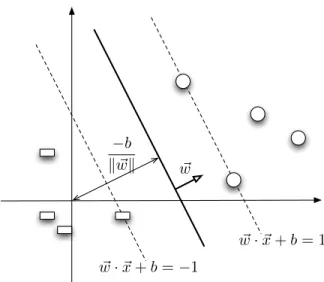
that it is going to rain, and −1indicates that it is not going to rain. The input features could be continuous measurements such as local atmospheric pressure, average/minimum/maximum temperatures, average humidity, or categorical features such as month and date in the year. Let us assume that there aredof such features (after suitable binarization of the categorical features). Suppose we have collected such data for the past year (n = 365), then we can regard these training examples as 365 points in ad-dimensional vector space, with la-bels+1 or−1over them. The concept of Support Vector Machines (SVM) as a binary classification algorithm is very simple: construct the most ”stable” linear hyperplane in thisd-dimensional space that separates the positive and negative examples (see Figure 2.2). This most stable hyperplane can be found by solving the following quadratic optimization problem:
Optimization Problem 2.1. (HARD-MARGIN BINARYSVM (PRIMAL)) min w∈Rd,b∈R 1 2kwk 2 s.t.∀i, yi(w·xi+b)≥1 (2.3)
The weight vector w is the normal of the hyperplane, and the scalar b is the offset of the hyperplane from the origin in the vector space. Note that the (signed) distance of the pointxifrom the hyperplane is kwwk·xi+kwbk (projection
onto unit normal). Therefore the constraintyi(w·xi+b)≥1is essentially
declar-ing that all the examples have to lie on the correct side of the hyperplane, with a minimum distance of1/kwk. Thus by minimizing the norm of w in the ob-jective, we are effectively maximizing the minimum distance to the hyperplane over all examples (called themargin).
However, for most of the training sets we receive for various classification problems, there do not exist any linear separators that have all positive
exam-! w ! w·!x+b=−1 ! w·!x+b= 1 −b "w!"
Figure 2.2: Binary Support Vector Machines
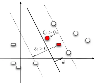
ples on one side and all negative examples on the other. This could be due to noise in the measurements, or simply that the features observed are not suffi-cient for confident prediction/separation of the two classes. In these cases the original quadratic optimization problems no longer have any feasible solutions, and we need to relax the linear constraints to allow feasible solutions. One way to do this is to introduce a non-negative slack variableξi for each example, to
allow the linear constraint to be violated by the amountξi (see Figure 2.3). The
optimization problem then becomes:
Optimization Problem 2.2. (SOFT-MARGIN BINARY SVM (PRIMAL)) min w∈Rd,b∈ R,ξ∈Rn 1 2kwk 2+C n X i=1 ξi s.t.∀i, yi(w·xi+b)≥1−ξi ∀i, ξi ≥0 (2.4)
The parameterCcontrols the trade-off between the two conflicting goals of having a larger margin and that of having smaller errors on the training set
! w ξi >0
ξj >0
Figure 2.3: Binary Support Vector Machine with Slack Variables
(sum of slacks). This is an important parameter for us to control overfitting to the training data.
To every minimization problem there is usually a closely related maximiza-tion problem called the dual problem (and the original one is called the primal). The values of the dual problem can be regarded as lower bounds of the val-ues of the primal problem. For most convex optimization problems under mild conditions (for example Slater’s constraint qualification or when the inequali-ties are all affine [15]) the value of the optimal primal solution and the value of the optimal dual solution coincide, a property which we callstrong duality. In those cases one can solve the dual optimization problem and recovers the pri-mal solution from that. The optimization problem for support vector machine is one such example where we can solve the dual problem. The dual optimization problem looks like the following:
Optimization Problem 2.3. (BINARY LINEAR SVM (DUAL)) max α∈Rn n X i=1 αi− 1 2 n X i=1 n X j=1 αiαjyiyjxi·xj s.t.∀i,0≤αi ≤C n X i=1 yiαi = 0 (2.5)
The variables αi are called the dual variables, and each αi corresponds to
exactly one constraintyi(w·xi+b)≥1−ξi in the primal. The primal and dual
solution are related by:
w =
n X
i=1
αiyixi, (2.6)
and thus we can easily recover the weight vectorwafter knowing all theαi’s.
Also the primal and dual variables have to satisfy the following complemen-tary slacknesscondition:
∀i, αi[1−ξi−yi(w·xi+b)] = 0.
One consequence of the complementary slackness condition is that when the constraintyi(w·xi+b)>1is satisfied strictly so that the slack variableξi = 0, the
corresponding dual variableαihas to be equal to 0. This is because[1−ξi−yi(w·
xi+b)]<0in this case andαi is forced to be 0 by the complementary slackness
condition. By Equation (2.6) examples(xi, yi)with dual variableαi = 0have no
effect in determining the expansion of weight vectorw, thus the solution of the optimization problem will remain the same if those examples are removed from the training set (examples lying outside the dotted line in Figure 2.3). Only those examples with dual variables αi > 0 can affect the solution of the SVM
optimization problem. These examples are calledsupport vectors, since they are like vectors exerting forces pushing towards (or supporting) the hyperplane,
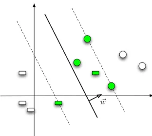
! w
Figure 2.4: Binary support vector Machine with slack variables, with sup-port vectors highlighted
and hence the name support vector machines. All the support vectors for the same problem as in Figure 2.3 are highlighted in Figure 2.4.
An interesting observation about the dual optimization problem in the above is that the only place where the input features enter the problem is through the inner productsxi ·xj. Vapnik and his colleagues, building on previous works
by [2], had the insight that these linear inner products can be replaced by more general functions onX × X called kernel functions to build complex nonlinear classification boundaries. The following is the dual SVM optimization problem with kernel functions:
Optimization Problem 2.4. (BINARY SVMWITH KERNELS (DUAL)) max α∈Rn n X i=1 αi− 1 2 n X i=1 n X j=1 αiαjyiyjK(xi,xj) s.t.∀i,0≤αi ≤C n X i=1 yiαi = 0 (2.7)
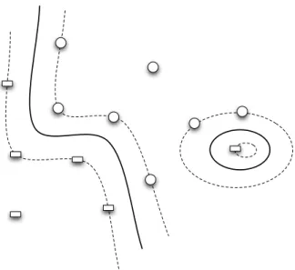
Figure 2.5: Binary SVM with Gaussian Kernels. The solid line is the deci-sion boundary, while the dotted lines are w·x = ±1. Notice the ability to introduce nonlinear and even disjoint decision re-gions using the Gaussian kernel.
Kernel functions are very general in the sense that they only need to sat-isfy a few conditions such as positive-semidefiniteness so that they can act like inner products for elements in X, but in a much higher and possibly infinite-dimensional space. Figure 2.5 shows the decision boundary with Gaussian ker-nels (or radial basis function kernel). Notice the nonlinearity of the decision boundary and also the ability have disjoint regions of the same class.
There is a whole body of theory on kernels in terms of Reproducing Ker-nel Hilbert Spaces [111], and numerous applications in areas such as computer vision [52, 148] and computational biology [112]. We will have a longer discus-sion on kernels in Chapter 6 when we talk about the use of nonlinear kernels in structural SVMs.
2.3
From Binary to Multi-Class Support Vector Machines
After a brief introduction to SVM let us consider the problem of how it might be extended for structured output prediction. For simplicity let us first assume we are working with a linear feature space.
The binary support vector machine is a very geometrically intuitive classifi-cation algorithm. Since there are only two possible output classes, finding the most stable hyperplane that separates the two classes as our decision bound-ary is a very reasonable idea. However, what should we do when the output
y is no longer binary, but contains multiple(> 2)different categories, or even exponentially many possible output classes as in structured output prediction?
Consider the case for classification when there is more than two output classes. It is no longer possible to have one separating hyperplanewthat cleanly puts all examples in one class withw·x>0and all other examples in the other class withw·x<0, since there are more than two classes (we are dropping the bias termb here for simplicity, and the effect of the bias term can be simulated by adding an extra constant feature in the examplesxi). Clearly to describe the
decision boundary we need more than one hyperplane w ∈ Rd, and it is not
clear what would be the most natural generalization of binary SVM.
Let us generalize from what we learn in the binary case. In general we have a linear decision scorew·xfor each examplex. The more positive the score is, the more likely will the example belong to the positive class; likewise the more negative the score is, the more likely for the example to belong to the negative class. Suppose there arek classes, we can set upk weight vectors such that the
decision score for theith class is:
wi·x
for1≤i≤k. To find out the most likely class for examplex, we compute argmax1≤i≤kwi·x.
The original binary SVM(k = 2)can be recovered by having the extra constraint w1 =−w2 to remove the extra degree of freedom.
Here we’re going to consider the multi-class SVM generalization by Cram-mer & Singer [35], since it poses the training problem as a single optimization problem without breaking the classification problem down into a series of bi-nary decision problems [106].
Optimization Problem 2.5. (MULTI-CLASSSVM (CRAMMER& SINGER)) min wc∈Rd,ξ∈Rn k X c=1 1 2kwck 2 +C n X i=1 ξi s.t.∀i,∀c6=yi wyi ·xi−wc·xi ≥1−ξi ∀i, ξi ≥0 (2.8)
We can notice that the objective function is essentially the same as binary SVM. The only difference comes from the constraints, which essentially says that the score of the correct labelwyi ·xhas to be greater than the score of any
other classes wc ·x, so there are k − 1 constraints in total when there are k
classes. There is one slack variableξi for each example, shared among thek−1
constraints.
We can simplify the notation by stacking the class weight vectors to form a single weight vectorw and introducing the notation for joint feature vector
Φ(x, y): w = w1 w2 .. . wk−1 wk ,Φ(x, y) = 0 .. . x .. . 0 ,
wherexappears in theyth block inΦ(x, y). Then the whole opimization prob-lem can be written succinctly as:
Optimization Problem 2.6. (MULTI-CLASSSVM (CRAMMER& SINGER)) min w∈Rkd,ξ∈Rn 1 2kwk 2 +C n X i=1 ξi s.t.∀i,∀c6=yi w·Φ(xi, yi)−w·Φ(x, c)≥1−ξi ∀i, ξi ≥0
2.4
From Multi-class to Structural Support Vector Machines
Structured output prediction problem, in its simplest form, can be regarded as a multi-class prediction problem, abeit with a huge number of classes in the output space Y (usually exponential in the input length). Consider the SVM formulation for structured output, which is a direct extension of the multi-class case:
Optimization Problem 2.7. (STRUCTURAL SUPPORT VECTOR MACHINES (MARGIN-RESCALING)) min w,ξ 1 2kwk 2+C n X i=1 ξi s.t.∀i,∀y¯∈ Y,y¯6=yi w·Φ(xi, yi)−w·Φ(xi,y¯)≥∆(yi,y¯)−ξi ∀i, ξi ≥0 (2.9)
The constraint essentially says that the score for the correct output w · Φ(xi, yi)has to be greater than the scorew·Φ(xi,y¯)for all alternative outputsy¯.
The loss function∆(yi,y¯)is new here. It controls the required margin between
the two scores, and in the case of multi-class classification it is 0 ifyi = ¯y, and 1
otherwise. The larger the value of the loss, the more differentyi and y¯are, and
the larger the required margin between them.
This optimization problem is still convex (convex objective with linear con-straints). While on the surface the training problem and the semantics of the constraints are quite similar to the multi-class case, the exponential size of the output spaceY makes a huge difference. For a start the constraint sets in struc-tural SVMs, unlike in the multi-class case, cannot be explicitly enumerated.
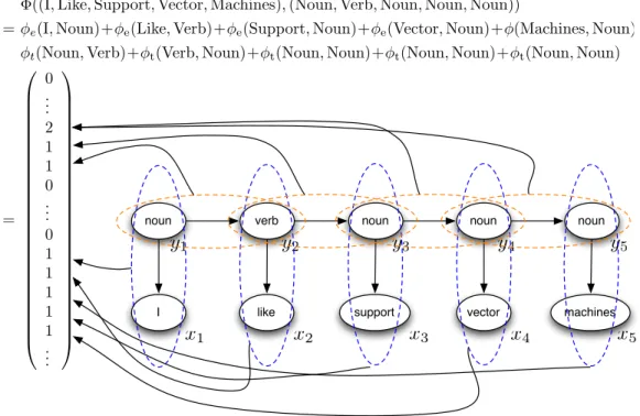
Let us now go back to the POS tagging example we have earlier in the be-ginning of the chapter. We can map the input ”I like support vector machines” and output ”Noun Verb Noun Noun Noun” to a high dimensional feature space with a joint feature mapΦ(x, y). This joint feature mapΦcan be constructed in many different ways. For example, one way is to have one parameter for each of the conditional probabilities in the conditional probability tables in Table 2.1 (see Figure 2.6). Notice how the the joint feature mapΦdecomposes into
emis-noun verb noun noun noun
I like support vector machines
x1 x2 x3 x4 x5 y5 y4 y3 y2 y1
Φ((I,Like,Support,Vector,Machines),(Noun,Verb,Noun,Noun,Noun))
=φe(I,Noun)+φe(Like,Verb)+φe(Support,Noun)+φe(Vector,Noun)+φ(Machines,Noun) φt(Noun,Verb)+φt(Verb,Noun)+φt(Noun,Noun)+φt(Noun,Noun)+φt(Noun,Noun)
= 0 .. . 2 1 1 0 .. . 0 1 1 1 1 1 .. .
Figure 2.6: Illustration of the joint feature mapΦapplied to the HMM ex-ample
sion featuresφe and transition features φt in Figure 2.6. In this way the score
w·Φ(x, y)will be like the logarithm of the joint probability in Equation (2.1). But unlike the generative HMM case these parameters are not to be directly in-terpreted as conditional probabilities, and they are also much less constrained. For example, the parameters corresponding to transitions and emissions do not have to sum to one for each hidden state. This approach is sometimes referred to as ”training a generative model discriminatively” in the literature [30].
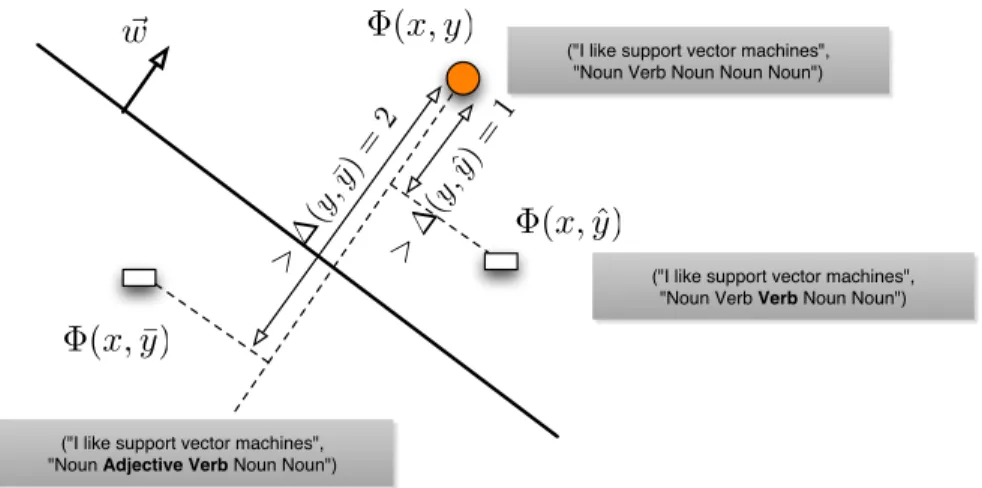
Figure 2.7 shows the visualization of what the constraints in the structural SVM formulation mean for our POS tagging example. The loss function ∆is the Hamming loss here. We want to find a direction or weight vector w that ranks the correct output ”Noun Verb Noun Noun Noun” the highest in the joint
!
w ("I like support vector machines",
"Noun Verb Noun Noun Noun")
("I like support vector machines",
"Noun Verb Verb Noun Noun")
("I like support vector machines",
"Noun Adjective Verb Noun Noun")
Φ(x, y) Φ(x,y)ˆ Φ(x,y)¯ >∆ (y, ˆ y)= 1 >∆ (y, ¯ y)= 2
Figure 2.7: Structural Support Vector Machine on POS tagging example
feature space. The alternative output ”Noun Verb Verb Noun Noun” mislabels ”support” as a verb and has a Hamming loss of 1, so the constraint requires it to be at least distance 1 (in terms of the linear scorew ·Φ(x, y)) away from the correct output. Another output ”Noun Adj Verb Noun Noun” in addition mislabels ”like” as an adjective and has a Hamming loss of 2. So the constraint requires it to be at least distance 2 from the correct output.
The number of constraints in the Optimization Problem 2.7 is exponential in the length L, and indeed there are kL ways to label a sequence of lengthL
when there arek different parts-of-speech. Having a constraint set size that is exponential in the input instance size is very common in structured output pre-diction problems. Obviously this rules out the option of solving the optimiza-tion problem by enumerating all the constraints. The optimizaoptimiza-tion problem can instead be solved by a cutting plane algorithm that generates constraints itera-tively (which we will talk about in greater detail in the next chapter), and each iteration involves computing:
In our POS tagging example, as long as the joint feature vector and loss func-tion decomposes linearly in hidden statesyi, then we can write the above
prob-lem as: argmaxyˆ∈Y L X j=1 [w·φe(x,yˆj) +w·φt(ˆyj−1,yˆj) +δ(yj,yˆj)], (2.11)
where δ(yj,yˆj) = 1 if yj 6= ˆyj, and is 0 otherwise (since the Hamming loss is
linear and∆(y,yˆ) = PLj=1δ(yj,yˆj)).
Notice that the structure of this argmax problem is exactly the same as the prediction problem we have in Equation (2.2), and thus can be solved by the Viterbi algorithm.
Moreover from Equation (2.11) we can see that the feature functionφe(x,yˆj)
can have arbitrary dependence on the whole input sequence x, unlike in the generative HMM case whereyˆj is only allowed to depend onxj due to the
con-ditional independence assumptions. Thus we can construct much more descrip-tive features such as havingyˆj depend onxj−1andxj+1 as well, or even a larger window of observations. Or we could construct other more global features such as the length of the input sequence. This extra flexibility of constructing arbi-trary features from the inputxis the major strength of discriminative modeling. Of course we also have to worry about overfitting when we introduce so many new features, but the regularization that comes with structural SVMs help con-trol it.
2.4.1
Kernels in Structural SVMs
Like binary classification SVMs, structural SVMs can also be ”kernelized” via the dual:
Optimization Problem 2.8. (STRUCTURALSVM (DUAL)) max α X i,yˆ ∆(yi,yˆ)αi,ˆy− 1 2 X i,yˆ X j,y¯ αi,yˆαj,y¯Φ(xi,yˆ)·Φ(xj,y¯) s.t. X ˆ y∈Y αi,ˆy =C αi,yˆ≥0 ∀i,∀yˆ∈ Y
The dual optimization only depends on the inner product of the joint fea-ture vectors Φ(xi,yˆ)· Φ(xj,y¯), and thus can be replaced by a kernel function
K(xi,y, xˆ j,y¯). In practice usually not the whole joint feature vector is mapped
nonlinearly to a high dimensional feature space, but only some constituient fea-ture functions such as emissions are replaced with polynomial or Gaussian ker-nels. We will discuss kernels in structural SVMs in details in Chapter 6.
2.4.2
Slack-rescaling
Apart from the structural SVM formulation that we discuss above, there is an-other version that uses a different penalization method for the slack variables, which is called slack-rescaling in the literature.
Optimization Problem 2.9. (STRUCTUALSVM (SLACK-RESCALING)) min w,ξ 1 2kwk 2 +C n X i=1 ξi s.t.∀i,∀y¯∈ Y,y¯6=yi w·Φ(xi, yi)−w·Φ(xi,y¯)≥1− ξi ∆(yi,y¯) ∀i, ξi ≥0 (2.12)
Here we assume that∆(yi,y¯)>0fory¯6=yi, so that the constraints are
well-defined. Compared to margin-rescaling we can see that the slack variable is penalized multiplicatively instead of additively by the loss. It would be even clearer if we re-organize the constraints:
ξi ≥∆(yi,yˆ)[1−w·Φ(xi, yi) +w·Φ(xi,yˆ)] (slack rescaling) (2.13)
ξi ≥∆(yi,yˆ)−w·Φ(xi, yi) +w·Φ(xi,yˆ) (margin rescaling) (2.14)
Slack-rescaling is less stringent than margin rescaling in the sense that as long as the score of the correct outputw ·Φ(xi, yi)is greater than the score of
any incorrect outputw·Φ(xi,yˆ)by 1 (or any fixed positive constant), then the
slack ξi will be 0. Notice that satisfying this condition is sufficient for
repro-ducing the correct output in the training set. On the other hand margin rescal-ing is more strrescal-ingent in specifyrescal-ing the exact margin requirements. In practice slack-rescaling usually performs better on noisy structured output prediction problems, since unlike margin rescaling alternative outputs with scores with less than the correct output have little effect on the slack variable. However, slack rescaling is usually more expensive computationally during training due to non-additive nature of the loss [109]. In this thesis we will focus more on the margin-rescaling formulation because of its computational advantages.
2.5
Bibliographical Notes
2.5.1
Related Models
Below we give a brief review of different machine learning methods that are closely related to structural SVMs in the area of discriminative structured output learning.
Conditional Random Fields
The influential paper by Lafferty, McCallum and Pereira [81] on Conditional Random Fields (CRFs) is the work that opens up the whole area of discrimi-native learning of structured output prediction models. Conditional random fields learn the conditional probability distributionP(y | x)with the following exponential form:
P(y|x) = Pexp(w·Φ(x, y)) ˆ
y∈Yexp(w·Φ(x,yˆ))
, (2.15)
whereΦis the joint feature vector that serves the same purpose as in structural SVMs, and w is the parameter vector to be learned. By modeling the condi-tional distributionP(y | x)instead of the joint distributionP(x, y), conditional random field is the first model that allows flexible feature construction in Φ, which greatly improves the performance of many sequence labeling tasks. No-tice in Equation (2.15) the normalization factor only involves summation over outputs yˆbut not inputx, and therefore one can construct arbitrarily complex feature over the inputxwithout having to worry about solving a more difficult inference problem in training. CRFs solve the following regularized negative log-likelihood minimization problem during training on a training set