Dissertations, Theses, and Masters Projects Theses, Dissertations, & Master Projects
2005
Application of survival analysis methods to pulsed exposures:
Application of survival analysis methods to pulsed exposures:
Exposure duration, latent mortality, recovery time, and the
Exposure duration, latent mortality, recovery time, and the
underlying theory of survival distribution models
underlying theory of survival distribution models
Yuan ZhaoCollege of William and Mary - Virginia Institute of Marine Science
Follow this and additional works at: https://scholarworks.wm.edu/etd
Part of the Biostatistics Commons, Environmental Sciences Commons, and the Toxicology Commons
Recommended Citation Recommended Citation
Zhao, Yuan, "Application of survival analysis methods to pulsed exposures: Exposure duration, latent mortality, recovery time, and the underlying theory of survival distribution models" (2005). Dissertations, Theses, and Masters Projects. Paper 1539616920.
EXPOSURE D URATIO N, LA TE N T M O R TA LIT Y , RECOVERY TIM E , AN D THE U N D ER LYIN G THEORY OF S U R V IV A L DISTRIBUTIO N MODELS
A Dissertation Presented to
The Faculty o f the School o f Marine Science The College o f W illiam and M ary in V irginia
In Partial Fulfillm ent
O f the Requirements fo r the Degree o f Doctor o f Philosophy
by Yuan Zhao
This dissertation is submitted in partial fu lfillm e n t o f the requirements fo r the degree o f
Doctor o f Philosophy
YtUlnA-
~ l£ u [> (y OYuan Zhao Approved, August 2005
M ichael C. Newman, Ph.D. M ajor Advisor/Committee Chairman
'S f
David A.^EyaftSTPhTD.
--- ^ - 1 ---r j T T Linda C. Schafrner, Ph.Yv
M ichael A. Unger, Ph.D.
’'Y'ISL
p
P hilip M . Dixon, Ph.D. Department o f Statistics
%
&
11
L.
i
m
X
A
*
A
%
%
€ AK
IPage
ACKNO W LEGM ENTS... v iii
LIS T OF TA B LE S ...ix
LIST OF FIGURES...x
ABSTRACT...xi
CHAPTER I. Introduction... 2
A. Current M etric o f Lethality in Ecotoxicology... 2
B. Survival Analysis Method... 5
C. Model Chemicals: Copper Sulfate and Sodium Pentachlorophenol... 11
D. Model Organism: Amphipod Hyalella azteca...14
E. Hypotheses to be Tested... 15
CHAPTER II. Incorporation o f Exposure Duration into Survival Analysis Models and Application o f the Models to Latent M o rta lity... 17
A. Introduction...17
B. Methods... 19
C. Results...23
D. Discussion...25
E. Conclusion...29
CHAPTER III. Pulsed Exposure: Effects o f Pulse Duration and Recovery Time between Pulses... 40
B. Methods... 42
C. Results... 45
D. Discussion... 48
E. Conclusion...52
CHAPTER IV . Test the Underlying Theory o f Dose-Response Model w ith Survival Analysis Methods...64 A . Introduction... 64 B. Methods...6 6 C. Results...69 D. Discussion...71 E. Conclusion...74
CHAPTER V. Summary and Conclusion... 84
APPENDIX 1...8 6 APPENDIX 2...87 APPENDIX 3...89 APPENDIX 4...91 APPENDIX 5...97 APPENDIX 6 ... 100 APPENDIX 7 ... 101 APPENDIX 8... 102 APPENDIX 9... 103 APPENDIX 10... 105
APPENDIX 12... 109
APPENDIX 13... 112
APPENDIX 14... 115
LITER ATU R E C ITE D ...116
It would not have been possible fo r me to finish this dissertation w ithout the assistance o f my committee members. Firstly, I would like to thank my major advisor, Dr. M ichael C. Newman, fo r his insightful guidance and great help throughout the course o f my study at VIM S. The knowledge and experience I learned from him is invaluable in my life . Dr. Michael A. Unger kindly provided me some experimental instruments fo r my research. His comments on my dissertation are also highly
appreciated. Dr. Linda C. Schaffner has given me many encouragements and advices, and is greatly acknowledged. I am grateful to my other committee members, Dr. David A. Evans and Dr. Philip M . Dixon, who provided me generous help on both the
statistics and experimental design.
I also would like to thank Dr. Harry V. Wang and Dr. Jian Shen, who have provided me various supports. M ary Ann Vogelbein taught me how to culture the experimental organisms, and Barbara Rutan helped me w ith the spectrophotometer operation. Since I came to V IM S, I received tremendous encouragements and help from my friends, Am y Shields, K ristin France, and Alanna M cIntyre, which are also highly appreciated.
Finally, I would like to thank my fam ily members - my grandparents, parents, brother, and husband - fo r their emotional support. Special thanks go to my husband, Taiping Wang, who was always my companion when I had to conduct overnight experiments.
Table
Page
2-1. The pH, DO, and water temperatures fo r the latent m ortality experiments...30
2-2. Concentrations o f Cu and NaPCP for the latent m ortality experiments... 31
2-3. AIC s and the best-fit models fo r CUSO4 experiments... 32
2-4. AICs and the best-fit models fo r NaPCP experiments... 34
3-1. The pH, DO, and water temperatures fo r the exposure duration and recovery time experim ents...53
3-2. Concentrations o f Cu and NaPCP for the exposure duration experiments...54
3-3. Concentrations o f Cu and NaPCP for the recovery time experiments...55
3-4. Percentages o f amphipods dead for the exposure duration experiments... 56
3-5. B est-fit models fo r exposure duration experiments... 57
3-6. B est-fit models fo r recovery time experiments o f CuS04... 58
3-7. B est-fit models fo r recovery time experiments o f NaPCP... 59
4-1. The pH, DO, and water temperatures fo r IED experiments... 76
4-2. Concentrations o f Cu and NaPCP o f IED experiments... 77
Figure
Page
2-1. Cumulative proportions o f amphipods dead fo r latent m ortality experiments 36
2-2. Conventional and complete LC50s... 37 2-3. Predicted proportion dead... 38 2-4. Response contours generated from survival models... 39
3-1. Cumulative proportions o f amphipods dead fo r exposure duration experiments 60
3-2. Cumulative proportions o f amphipods dead fo r recovery time experiments...61 3-3. Time-to-death for a certain proportion o f animals to die... 62
3-4. Observed and predicted times-to-death o f the different recovery time groups 63
4-1. Hypothetical plots o f cumulative m ortality under IED and stochastic theory 79
4-2. Cumulative proportion mortalities fo r CUSO4 IED experiments... 80
4-3. Cumulative proportion m ortalities fo r NaPCP IED experiments... 81 4-4. Cumulative mortalities during the firs t part o f the second lethal NaPCP exposures..82 4-5. Cumulative m ortalities during the second part o f the second lethal NaPCP exposures
Ecotoxicologists adopted median lethal concentration (LC50) methods from mammalian toxicology. This conventional LC50 approach has shortcomings in spite o f its expediency and convenience. Fixing the exposure duration and selecting the 50% m ortality level result in loss o f ecologically relevant inform ation generated at all other times. It also ignores latent m ortality that can manifest after exposure ends. As a result, the conventional LC50 approach cannot adequately predict pulsed exposure effects in which concentration, duration, and frequency o f pulses change through time.
Furthermore, the underlying theory o f the dose-response models used to calculate LC50 values, stochastic versus individual effective dose (IED ) theory, has not been tested rigorously, w hile a better understanding o f it is needed in order to better predict the effects o f pulsed exposures.
In this study, the effects o f exposure duration and concentration on m ortality during and after exposures, and the effects o f recovery time between two pulses on m ortality during the second pulse were quantified. The influences o f toxicant modes o f action on latent m ortality were discussed. The underlying explanation fo r survival distribution models was further explored. Survival analysis methods were used to incorporate these factors affecting m ortality during pulsed exposures into predictive models and to circumvent some o f the shortcomings o f the conventional LC50 method. The experiments were done w ith two notionally contrasting toxicants, copper sulfate
(CUSO4) and sodium pentachlorophenol (NaPCP). The amphipod, Hyalella azteca, was used as the model organism.
Latent m ortality is an integral part o f the lethal effects o f some toxicants that cause cumulative damage. Exposure concentration has a significant effect on latent m ortality. For toxicants that cause m inim al damage during the exposure, the latent m ortality is not significant and can be potentially ignored. Exposure duration did not show any significant effect on latent m ortality w ithin the experimental ranges fo r either toxicant. It is recommended that fo r other experimental conditions the effect s till needs to be considered. Recovery time between two pulses had significant effect on m ortality during the second pulse fo r both toxicants. However, to recover to a sim ilar background level m ortality, the time an exposed organism needed to return to a stage sim ilar to its
original resistance was much longer fo r Q1SO4 than fo r NaPCP. The hypothesis that
individual effective dose is the dominant explanation fo r the dose-response models was rejected fo r both toxicants. By effectively incorporating exposure duration and other factors into the models, the application o f survival analysis methods better predicted pulsed exposure consequences than did the conventional LC50 method. It is im portant fo r current ecotoxicology and environmental risk assessment to consider the factors potentially affecting pulsed exposure consequences. The survival analysis provides a better way to address the issue.
EXPOSURE D URATIO N, LA TE N T M O R TA LITY , RECOVERY TIM E , AN D THE U ND ER LYIN G THEORY OF S U R V IV A L D ISTR IBU TIO N MODELS
CHAPTER I. INTRODUCTION
A. Current M etric o f Lethality in Ecotoxicology
The current use o f the median lethal concentration or dose approach
(LC50/LD50) to measure chemical to xicity in ecotoxicology has its roots in classic mammalian toxicology. H istorically, researchers quantified to xicity by defining
threshold concentrations for toxicants using a fixed exposure duration but found that the high uncertainty in predictions at the lower ta il o f the dose-response curve made
estimation too imprecise. Finney (1947) argued that the 50% response level should be used instead because the associated estimates o f lethal concentrations at 50% exhibit less variability than those at higher or low er percentiles. The LC50/LD50 became the metric o f to xicity in mammalian toxicology.
From the mid-1940s, environmental toxicologists began to adopt this approach for their use in laboratory bioassays, using the results to im ply environmentally safe concentrations (Cairns and Pratt 1989). Experimental organisms are exposed to a series o f toxicant concentrations and their percentage mortalities are recorded at the end o f an experiment. Exposure durations are grossly defined as acute (e.g., 48 h or 96 h) or chronic (e.g., 10% or more o f the species’ life span). These time-endpoint methods are used to evaluate the chemical concentration producing a specific level o f effect such as the 96 h LC50. This method is fast and simple to perform, and insensitive to violations o f statistical assumptions, e.g., assuming either a log-normal or log-logistic distributed
model w ill result in sim ilar LC50 values (Dixon and Newman 1991). During early applications o f these methods, people adequately predicted to xicity associated w ith point sources and compared the relative toxicities o f different toxicants or different species o f the same toxicant. However, there was and s till is a tendency to uncritically apply these routine toxicity test protocols to situations in which they have important shortcomings.
Toxic effect is a function o f both exposure duration and intensity (concentration or dose). In general, the higher the exposure concentration or the longer the duration, the more damage that is caused. However, environmental regulators tend to focus on concentration while considering duration peripherally. The duration o f a LC50 test is set based on convenience, e.g., 96 h fits conveniently w ithin a work week, not ecological relevance. Exposure durations differing from 96 h are like ly and the 96 h LC50 w ill im perfectly predict m ortality fo r these other durations. Scoring m ortality only at the end o f the exposure period results in lose o f valuable inform ation generated for other
ecologically relevant times. For example, w ith the 96 h LC50 o f dissolved Cu o f a fish species, we can neither quantitatively predict the proportion o f fish dead at 48 h, nor if the fish population w ill be viable after the 96 h Cu exposure.
In the context o f predicting ecological consequences, the statistically most precise 50% point has questionable biological significance. In many situations,
concentrations resulting in lower or higher percentage mortalities can be meaningful to determine risk upon toxicant released and helpful fo r regulators while setting toxicant standards in the environment.
Conventional endpoint tests also do not address lethal effects that happen after exposure ends (latent m ortality). In mammalian toxicology, the LC50 method is designed to measure toxic effects on individuals; in ecotoxicology, the prim ary interest is to predict the fate o f a field population after exposure. Latent m ortality could be an integral component o f the exposure consequences (e.g., Newman and McCloskey 2000, A rthur 2001, Cerqueira and Fernandes 2002). To quantify latent m ortality, observation must continue after the exposure ends. Noting m ortality only at the end o f exposure compromises the usefulness o f the associated lethality predictions.
In reality, organisms experience pulsed exposures in which exposure
concentration, duration, and frequency change through time. The conventional toxicity tests are derived fo r an exposure scenario o f fixed durations and constant concentrations, and cannot accurately model pulsed exposure. Pulsed exposures norm ally occur after events such as m ultiple pesticide sprayings, snowmelt or rainstorms follow ing dry periods, repeated discharges, or tidal fluctuation in an estuary. Chemicals, especially agrochemicals, occur at different sub-lethal concentrations for most o f the time w ith potentially lethal concentrations being reached periodically. The assessment o f these pollutant effects requires more than the conventional concentration-response methods provide.
Finally, people tend to use the LC50 metric as a measure o f to xicity w ithout paying sufficient attention to its underlying mechanism. A probit (log-normal) model is assumed in most analyses o f dose-response data. The dominant explanation o f this log normal distribution is the individual effective dose (IED ) theory: each individual has a characteristic tolerance fo r the toxicant and w ill die i f the exposure dose or
concentration exceeds its IED (Gaddum 1953). The IED values are thought to be log- normally distributed w ithin a population. This IED concept permeates interpretations o f other models o f acute lethality as well. However, it has not been rigorously tested before Newman and McCloskey (2000) and may not be a sufficient explanation fo r all, or even most, applications o f the model. A plausible alternative explanation is a
stochastic one: at a specific concentration, all exposed animals have the same chance of dying and which specific individual w ill die is determined by a random process defined commonly by a log-normal (or skewed) model (Berkson 1951). To determine the correct explanation fo r the probit and sim ilar models is important in predicting population fate after pulsed exposures. Under the IED theory, the survivors o f the exposures are more robust than the dead ones but, under the stochastic theory, there is no difference between the dead and the survivors. W ith a same exposure scenario o f repeated pulses, a population would persist much longer if the IED theory were true rather than i f the stochastic theory were.
B. Survival Analysis Method
The survival analysis method was applied in this dissertation to overcome several shortcomings o f the LC50 methods mentioned above. The survival analysis method is also called time-to-event, survival time, or failure time analysis. It was in itia lly developed in medical sciences and engineering. In agricultural sciences, it has been applied to insect pathology. This includes the study o f m ortality when insects are challenged by pathogenic microorganisms (e.g., Fenlon 2002). In engineering, it has been used in re lia b ility testing o f components and systems where the event o f interest is
usually failure o f the component or degradation o f system performance (e.g., Kim ber 2002). F ully parametric models are usually used in engineering because good predictive models fo r the failure time distribution are valued. In the medical field, it is used to predict the effects o f various variables on survival o f animals or humans. Semi-
parametric models are often used i f researchers are more interested in relative effects o f different treatments, not the exact failure time. For example, in the classic Stanford Heart Transplant experiment (Crowley and Hu 1977), the Cox semi-parametric model was used to study whether transplantation raised or lowered the risk o f death w ith covariates such as date o f birth and age o f acceptance included in the study. Other applications in medical, engineering, and other fields can be found in text books (e.g., Crowder et al. 1991, Ansell and Phillips 1994, C ollett 1994, A llison 1995, Cantor 2003).
Only recently has survival analysis been applied to environmental risk assessment and ecotoxicology. Survival time modeling was applied to acute NaCl toxicity data fo r the mosquitofish, Gambusia holbrooki (Newman and A p lin 1992). Both concentration and fish wet weight were included in the model. The authors suggested consideration o f this method as an adjunct to conventional to xicity testing endpoints. A population o f rainbow trout was challenged w ith viral haemorrhagic septicaemia (VHS) and the survival function was estimated by assuming a W eibull distribution (Henryon et al. 2002). Honeybee (Apis mellifera ligustica) survival after chronic exposure to the insecticides, deltamethrin and im idacloprid, has been studied with survival models (Moncharmont et al. 2003). The time required fo r an individual
amphipod (Leptocheirus plumulosus) to burrow below the sediment-water interface was
amphipod burrowing behavior is sensitive to sediment contamination. Survival analysis was used to evaluate the effect o f the number o f infected fish and acute exposure on the development o f branchial xenomas during a Loma salmonae infection (Becker et al. 2005).
The general approach o f survival analysis involves exposing organisms to toxicant solutions and monitoring the effects (e.g., m ortality, lose o f equilibrium , hatch, sexual m aturity, or spawn) through time. Non-responders (e.g., survivors) are treated as statistically censored because their exact times-to-event are unknown. Maximum likelihood estimations (M LE) are conventionally used to analyze the data because o f this censoring.
Some terminologies are im portant and frequently used in survival analysis. The m ortality o f individuals can be described w ith a cumulative distribution function (cdf), F(t), or probability density function (p d f),/(f). The cdf at a certain time T is a function o f the probability that the variable w ill be less than or equal to any value t that we choose: F(t) - P(T < t). An estimate o f the F(t) would be the total number o f individuals dead at time, t, divided by the total number o f individuals exposed to the toxicant:
r,/ , Number Dead (t) ... ,,
F it) =--- —— (1.1)
Total Number Exposed The pdf is the derivative or slope o f the cdf curve:
/ « = ^ (1.2)
at
The survival function S(t) describes the probability o f surviving beyond time t. It is estimated by the number o f individuals surviving to time t divided by the total number o f individuals exposed to the toxicant:
The hazard function h(t) is used to describe the instantaneous death rate at time t conditioned on the organism’s survival to time t:
Pit < T < t + A t\T > t) f(t)
h(t) = l i m ^ --- !--- ^ = ^ (1-4)
aj->o At S (t)
The cumulative hazard function H(t) is the integral o f the hazard function:
t
H ( t ) - ^ h(t)dt - - ln ( l - F(t)) (1.5)
o
Nonparametric, semi-parametric, and fu lly parametric methods are available fo r analyzing these data. Nonparametric methods include product-lim it and life-table methods, and do not require a specific distribution fo r the survival curve. Survival for different groups o f exposed individuals can be tested fo r equality w ith the
nonparametric log-rank or W ilcoxon test. The general form o f the semi-parametric and parametric models is:
/* (f, jcO = e f(xi) h0 ( t , e nx'} ) (1.6)
where h (t, jq ) is the hazard function fo r group x,; ho (t, ef (Xi)) is the baseline hazard at time t fo r group xr, ef (Xl) is a function that relates the hazard to the baseline hazard; and/ (xi) is a function o f either continuous variables such as concentration, or class variables such as sex. For a semi-parametric proportional hazards model, the distribution o f baseline hazard ho (t, ef (X|)) does not need to be specified. The hazard o f a treatment group is some m ultiple o f the baseline hazard. For a parametric model, Equation 1.6 can be rearranged to the form o f an accelerated failure time model:
where l\ is the tim e-to-event,/( X j) is a function that relates the covariates to and e, is the error term, which fo r prediction purposes is a x L. The L varies w ith the proportion dead fo r which prediction is being made and can be obtained from the Table 7 of
Newman (1995). The scale parameter a defines the scale o f the hazard curve. The ti w ill have a W eibull, exponential, log-logistic, or log-normal distribution i f e, is assumed to have either the distribution o f extreme value w ith two parameters, extreme value w ith one parameter, logistic, or normal, respectively (Cox and Oakes 1984). I f the numbers o f parameters fo r the four candidate distributions above were the same, the log
likelihood statistic associated w ith each distribution could be applied directly to select the best-fit model. Larger log likelihood value indicates better fit. I f the numbers o f parameters d iffe r among candidate models, A kaike’ s inform ation critierion (A IC ) can be used (Atkinson 1980):
A IC - -2 x (log likelihood statistic) + 2 x (number o f parameters) (1.8)
It favors parsimony in selecting among models. Lowest A IC values indicate the best- fittin g and parsimonious model, i.e., the model w ith the most inform ation per estimated parameter.
Survival analysis has many advantages relative to the conventional LC50 method, including:
1) Survival analysis can include exposure duration, a crucial determinant o f toxic effect, into the model.
2) More data can be produced from it than from the conventional LC50 method. Therefore, statistical power is greatly enhanced (Newman and Dixon 1996, Dixon
3) Because o f the increase o f statistical power, important covariates associated w ith the exposure such as concentration, temperature, and pH value can be included in the models and their effects quantified. Also, because times-to-death are recorded fo r individuals, covariates associated w ith individuals such as sex, age, and body weight can be included in predictive models more effectively.
4) Time-to-event results can be applied directly in ecological, demographic, and epidemiological models. For example, i f the time-to-death and time-to-reproduce are monitored fo r a fish population exposed to a toxicant, the number o f young bom (mx) and proportion o f individuals dying (lx) can be generated. W ith mx, lx, and the original number o f a fish population, the Leslie m atrix approach (Leslie 1945, Caswell 1996) can be used to predict population qualities and fate through time (Newman and McCloskey 2002).
5) The conventional endpoint estimates, such as LC50, and the associated confidence intervals can be estimated as w ell from survival models. More precise prediction can result in many (but not all) cases (Dixon 2002).
The advantages o f survival analysis allow us to potentially overcome many o f the shortcomings o f conventional LC50 methods, especially to predict pulsed exposure effects more effectively. Firstly, both exposure duration and concentration can be included in the model and their effects predicted. Secondly, latent m ortality and the variables affecting latent m ortality can be quantified. Thirdly, lethal effect o f pulsed exposure may be quantitatively predicted by incorporating form er exposure
model. Last, the underlying mechanism o f log-normal and sim ilar models can be further explored.
C. Model Chemicals: Copper Sulfate (CuSCL) and Sodium Pentachlorophenol (NaPCP) Copper sulfate and NaPCP were selected because their different modes o f action on aquatic animals and anticipated contrasting latent effects. Copper can cause
cumulative damage to g ills and the exposed animals w ill like ly need a long period o f time to recover and the latent m ortality m ight be high. For NaPCP which causes less cumulative damage, the exposed animals have a good chance o f recovery after exposure ends and the latent m ortality m ight be low. Because latent m ortality is an integral, albeit often ignored, consequence o f pulsed exposure, the effects o f the two toxicants during pulsed exposure could be different as well. Furthermore, the two toxicants can be representative o f two contrasting modes o f action, and the underlying dominant theory (IED versus stochastic) for probit and sim ilar models m ight be different. Their uses, environmental fates, and toxicities are b rie fly discussed below.
1. Copper and copper sulfate
Copper sulfate is used to control bacterial and fungal diseases o f fruits,
vegetables, nuts, and fie ld crops. It is also used as an algaecide and herbicide, and to k ill slugs and snails in irrigation and m unicipal water treatment systems.
Copper can be bound or adsorbed to organic material, and to clay and mineral surfaces. The degree o f adsorption to soils depends on soil acidity or alkalinity. It is considered one o f the more mobile metals in soils. Because o f its binding capacity, its
leaching potential is low in all but sandy soils. Applied w ith irrigation water, C uS04
does not accumulate in the surrounding soils. About 60% deposits in the sediments at the bottom o f the irrigation ditch, and becomes adsorbed to clay, mineral, and organic particles (U.S. National Library o f Medicine 1995).
Copper sulfate is highly toxic to fish. Even at recommended rates o f application, this material may be poisonous, especially in soft or acid waters. Its to xicity generally decreases as water hardness increases. It is toxic to aquatic invertebrates too. Some amphipod species are especially sensitive to it. Copper inhibits Na+/K + ATPase activity and induces chloride cell necrosis and apoptosis. It increases g ill membrane
permeability and chloride cell dysfunction. In the end, the osmotic and ionic functions o f g ills are disrupted (Cerqueira and Fernandes 2002). The prevalence o f lesions depends on the chemical concentration and exposure duration, and the tissue recovery depends on the severity o f the damage and the environmental conditions (Poleksic and M itrovic-Tutundzic 1994). Copper also bonds between heterocyclic bases o f D NA, competes w ith the normal hydrogen binding, and destabilized the D N A structure (Eichhom 1975). Therefore, organisms may need relatively long periods o f time to recover depending on the cumulative damage caused during exposure. Studies (e.g., Icely and N ott 1980, Caparis 1989, Eriksson and Weeks 1994) have shown that
amphipods can accumulate significant amount o f Cu by storing it in granules o f midgut. Metallothioneins and m etallothionein-like proteins can be induced by Cu, thus reduce the amount available to cause a toxic effect on amphipods.
2. Pentachlorophenol and sodium pentachlorophenol
Sodium pentachlorophenol’ s greatest use is as a wood preservative. It was banned fo r herbicide use in 1987. Other uses include soil fumigation fo r termites, seed treatment fo r beans, antibacterial agent in disinfectants/cleaners, and preservative for glues, starches, and photographic papers (EPA fact sheet 2003).
Pentachlorophenol and NaPCP may be released to the environment as a result of its production, storage, transport, or usage. In air, PCP w ill be degraded through
photolysis. A ny PCP released to soils w ill slow ly biodegrade and leach into
groundwater. It tends to adsorb to soil and sediment, and the adsorption is stronger under acid conditions. Evaporation from water is slow, especially at natural pH values. It does not appear to oxidize or hydrolyze under environmental conditions (EPA fact sheet 2003).
Hedtke et al. (1986) conducted PCP acute freshwater to xicity tests on the amphipod, Crangonyx pseudo gracilis, obtaining 96 h LC50 values o f 0.32, 0.22, and
1.55 m g/L in different periods during the summer. Juvenile amphipods, Gammarus
psuedolimnaeus and Crangonyx pseudo gracilis, were exposed to PCP at different pH values and PCP toxicity decreased w ith increased pH (Spehar et al. 1985).
Pentachlorophenol is expected to bioconcentrate in organisms and the bioconcentration factor (BCF) w ill be dependent upon the pH o f the water because PCP w ill be more dissociated at higher pH values (EPA fact sheet 2003). The toxicological mode o f action o f PCP is increased cellular oxidative metabolism resulting from the uncoupling o f oxidative phosphorylation. It tends to diffuse across the g ill from the amphipod’ s body
(Spacie and Hamelink 1985). It was found that the clearance rate increases as salinity increases (Tachikawa and Sawamura 1994). It can be converted directly by phase II conjugation reactions at a faster rate than contaminants that are transformed by oxidative metabolism w ith cytochrome P450. Therefore, after it is removed from the environment, the toxic effect is reversible and the cumulative damage after the exposure may not be as prominent as that o f Cu. Organisms exposed to PCP could acquire
increased tolerance through acclimation (e.g., Norup 1972).
D. Model Organism: Amphipod Hyalella azteca
The freshwater amphipods H. azteca were used as experimental animals. Amphipods are one o f the orders in the subphylum Crustacea and class Malacostraca. The genus Hyalella belongs to the order Amphipoda and fam ily Hyalellidae (Voshell 2002). They are bottom dwellers in small spaces, such as cool streams, springs, and ponds, coarse detritus, or upper layer o f soft sediment.
The normal body length o f adult H. azteca is 8 mm fo r males and 6 mm for
females. Body color is a creamy light gray and somewhat translucent. It is omnivorous but its most common food is detritus. It also grazes on algae, fungi, and bacteria. It completes its life cycle in 27 days or longer depending on the temperature and die w ithin one year. Individuals that live in waters where temperatures change seasonally usually reproduce in spring and summer. Bovee (1950) and Sprague (1963) found temperatures tolerated by H. azteca range from 0 to 33 °C.
Amphipods are nearly ubiquitous in permanent fresh waters o f the New W orld. They are im portant items in the diet o f many invertebrates, fish, amphibians, and water
birds. They are important in the breakdown o f particulate organic matter. The amphipod H. azteca has many desirable characteristics as an experimental organism including short generation time, ease o f culture, relative sensitivity to contaminants and tolerance o f varying physical-chemical properties o f environments, and an easily identifiable m ortality end point. Therefore, it became one o f the EPA recommended species for assessing acute toxicity o f freshwater sediment (EPA 2000). However, in a recent study, Wang et al. (2004) suggested that because o f the gap between laboratory and nature, it is probably a suitable surrogate species fo r determining sediments that are lik e ly not toxic to fie ld populations, while not suitable fo r determining sediments that are like ly toxic to fie ld populations.
In a study conducted on H. azteca (De March, 1978), higher temperatures produced smaller animals. Higher temperatures and longer photoperiods increased reproductive activity o f the species (Kruschwitz 1978). The survival, growth, and reproduction o f H. azteca were determined under various test conditions (Borgmann et al. 1989). There have been numerous studies w ith H. azteca on acidification (e.g., Grapentine and Rosenberg 1992, France 1996), and toxicity (e.g., M orris et al. 2003, Borgmann et al. 2005) and bioaccumulation (e.g., Jessiman and Qadir 1983, Burton et al. 2005) o f various toxicants.
E. Hypotheses to be Tested
Based on the lim itations o f current LC50 method, the advantages o f survival analysis method, and the need to predict lethal consequences o f pulsed exposures, I established the follow ing four hypotheses fo r my dissertation:
conventional LC50 method. It more e fficie ntly includes time, concentration, and other important covariates into predictive models.
Hypothesis 2: Survival analysis allows statistical testing fo r and effective quantification o f latent m ortality.
• For CuS04, cumulative damage to g ills and other tissues causes high latent m ortality and the m ortality is a function o f previous exposure concentration.
• For NaPCP, reversible and less pervasive cumulative damage causes insignificant latent m ortality and the m ortality is relatively independent o f previous exposure concentration.
Hypothesis 3: Survival analysis permits more effective prediction o f lethal effects from pulsed exposure.
A fter the prelim inary experiments and the results o f Hypothesis 2, the follow ing sub-hypotheses o f Hypothesis 3 were established:
• For CuS04, there is significant effect o f previous pulse duration on latent m ortality, and the effect can be quantified; fo r NaPCP, there is not significant effect o f pulse duration on latent m ortality.
• For both CuS04 and NaPCP, there are significant effects o f recovery
time between the two pulses on m ortality during the second pulse. Hypothesis 4: The IED theory is the sole or dominant explanation fo r the
CHAPTER II. INCORPORATION OF EXPOSURE D URATIO N INTO S U R V IV A L AN ALYSIS MODELS AND APPLICATION OF THE MODELS TO LATEN T
M O R T A LIT Y
A. Introduction
In a variety o f fields such as medical sciences and engineering, duration is commonly included as one of the variables in the statistical models described in Chapter I. In ecotoxicology, scientists began including exposure duration in their models from the beginning o f the last century. One o f the first applications was a rectangular
hyperbola-like survival curve for Daphnia (Warren 1900). The times-to-death and percent mortality data o f tuberculoid mice were fit to log-probability paper, and a median lethal time (LT50, the predicted exposure time needed to get 50% mortality at a preset concentration) o f 46 d was calculated (Litchfield 1949). Herbert and Merkens (1952) generated a log concentration versus log survival time graph for rainbow trout in potassium cyanide solutions. The linear range was expressed as C " x T - k, where C was concentration, T was survival time, and n and k were estimated parameters. Burdick (1957) expanded the model to (C-a) ” x (T-b) - K, where a and b were the threshold concentration and time, respectively. Jones (1964) found that survival time increased as concentration decreased until a point was reached where it became indefinitely long (the threshold concentration), and as concentration increased, a stage could be reached when further increases in the concentration would not materially shorten the survival time (the
threshold reaction time). In order to normalize discrete atrazine exposure data for irregular sampling, a crude moving window technique was used more recently to approximate the 4-d and 21-d average atrazine effect concentrations (Solomon et al. 1995). Mayer et al. (1994) described a two-step linear regression approach that uses acute lethal data to estimate chronic toxicity with exposure time as an independent variable. The predicted no-observed-effect concentration (PNOEC) was estimated from the regression. Based on this and another two methods (accelerated life testing and multifactor probit analysis), the Acute-to-Chronic Estimation software (Ellersieck et al. 2003) was developed to predict long-term toxicity with data from short-term
experiments. A ll o f the methods described in this paragraph provide gross predictions o f the influence o f exposure duration.
Though many scientists made efforts to include time into their toxicological models, most have restricted their attention to times during the exposure. Latent
mortality is not routinely quantified and reported in lethality studies. Pascoe and Shazili (1986) observed significant post exposure mortality resulted from brief cadmium exposure. The term median post exposure lethal time (peLT50) was proposed as a means o f assessing and comparing the results o f brief exposure to a pollutant. Reinert et al. (2 0 0 2) suggested that, in order to demonstrate latency (or lack o f latency),
observation intervals should be continued after the exposure ends.
Latent mortality could be affected by several variables such as life stage o f the exposed organisms, the toxicant to which the organisms are exposed, exposure
concentration, exposure interval, and temperature. Guadagnolo et al. (2000) found that rainbow trout eggs were more sensitive after silver exposures during certain
development periods than during other periods. Arthur (2001) found grain beetle mortality after the initial exposures to wheat treated with diatomaceous earth increased as exposure interval and temperature increased. Newman and McCloskey (2000) observed mosquitofish latent mortality extended for 3 to 4 weeks after NaCl exposure,
but only 8 h after PCP exposure. Naddy et al. (2000) found daphnids did not experience
any delayed effects from chlorpyrifo exposures up to 20 d after exposure. The difference may be because the effects are reversible unless death has occurred for substances that display a baseline or narcotic mode o f action (Reinert et al. 2002). None o f these studies formally quantified the relationship between the degree o f latent
mortality and variables that could potentially affect it.
In the current study, the amphipod, H. azteca, was exposed to different CuSC>4
and NaPCP concentrations. Time-to-death data taken during and after the exposures were fit to survival models. By including exposure duration and concentration as covariates in the models, the proportion dead was predicted at any concentration and any exposure time within the experimental range. By comparing the conventional 48 h LC50 and the complete LC50 values (defined as the LC50 values calculated by
including mortalities during and after exposure ends) and contrasting the latent effects o f the two toxicants, the importance o f including latent mortality into ecotoxicological models was demonstrated.
B. Methods
The amphipods, H. azteca, came from a population that had been maintained in our laboratory for more than two years and never experienced contaminant exposure. W ell water was used as the culturing water and red maple (Acer rubrum) leaves as food. Test amphipods were one to two weeks old and were obtained by gently siphoning water from the cultures onto screens. The amphipods that passed through a 0.67 mm sieve but were retained by a 0.50 mm sieve were used as test organisms. They were maintained in the reformulated moderately hard reconstituted water (RMHRW ) (Smith et al. 1997) with food at 23°C for at least 72 h before the exposures began. The
chemicals needed to prepare RMHRW and the expected alkalinity and pH ranges are listed in Appendix 1.
2. Exposure procedure
Several range-finding tests were conducted to determine the concentrations to be used in the following formal experiments. Three CuSCE exposures were conducted in January, February, and July 2003, respectively. Copper sulfate was dissolved in RMHRW to make five solutions with nominal dissolved Cu concentrations o f 0.0, 0.2, 0.3, 0.4, 0.6 mg/L. Each solution was delivered to four 12-well COSTAR 3513 Cell Culture Clusters (Corning, Coming, NY, USA) with approximately 4 ml in each well. Two hundred and forty amphipods were then randomly assigned to the wells with one animal per well. Each well contained a piece o f red maple leaf as food (leaf weight in each well: 0.61 ± 0.32 mg, mean ± standard deviation, n = 40). Every amphipod exposed to the same concentration was considered a replicate. The cluster plates were then placed in a LA B -LIN E A M B I-H I-L O Chamber (Lab-Line Instruments, Melrose
Park, IL, USA). M ortality was checked at approximately 4 h intervals. An amphipod was scored as dead and removed from the well i f no sign o f appendage movement was discernible after gentle prodding. A ll the amphipods alive after 48 h were carefully transferred to fresh RMHRW. Latent mortality was noted approximately every 4 h. The experiment ended at 112 h when no more mortality was evident. A ll the survivors after that time were noted as right-censored. During all the experiments, 48 amphipods were established as control animals and maintained in water free o f toxicant.
Three NaPCP exposures were conducted in early June, mid-June, and late July o f 2003, respectively. Sodium pentachlorophenol was dissolved in RMHRW to make solutions with nominal NaPCP concentrations o f 0.0, 0.2, 0.3, 0.5, 0.8 mg/L. The
exposure and post exposure procedures were the same as those o f Q1SO4. The only
difference was that the experiments ended at 85 h, when no more latent mortality was evident. Forty eight amphipods were established as control animals as well.
The total alkalinity and pH o f RM HRW were measured before exposures started to ensure that they were within the expected ranges. The solutions were renewed during the experiments every 12 h. Both newly prepared and 12 h-exposed water samples were collected for pH and toxicant concentration measurements. The pH values were
measured with an ACCUM ET M odel-15 pH Meter (Denver Instrument, Denver, CO, USA) and PerpHect ROSS Electrode Model 8256 (Orion Research, Boston, M A , USA). Water samples for dissolved Cu measurement were acidified, stored at 4 °C, and
analyzed with a Perkin-Elmer AAnalyst 800 atomic absorption spectrometer (Perkin- Elmer, Norwalk, CT, USA). Samples for NaPCP analysis were collected with glass bottles, stored in 4°C, and analyzed with the method o f Carr et al. (1982). Each 25 ml
water sample was mixed with 25 ml de-ionized water and 0.5 ml o f concentrated HC1. Ten ml o f chloroform was added before the sample was shaken vigorously for 60 s. Five ml o f the extract was collected in a polypropylene centrifuge tube. Two ml o f 0.2 M NaOH were added to the extract, mixed vigorously for about 30 s, and centrifuged in an IEC H N-SII Centrifuge (International Equipment, Needham Heights, M A , USA) at 5000 G for 5 min. The absorbance o f the aqueous fractions was measured with a Beckman DU 650 spectrophotometer (Beckman Instruments, Fullerton, CA, USA) at 320 nm. Samples for temperature and dissolved oxygen (DO) were taken periodically and measured with a Fisher mercury thermometer and YSI Model 57 oxygen meter (YSI, Yellow Springs, OH, USA), respectively.
3. Data analysis
The exposure concentration, total number o f exposed amphipods, and number o f dead amphipods were fit to a probit model with logio transformation o f concentration to calculate the conventional 48 h LC50 and complete LC50 values. The associated 95% fiducial lim its were calculated as well (TOXSTAT® 1989).
The parametric accelerated failure time model was used to analyze the survival data with toxicant concentration as the independent variable:
In t{ = / ( concentration) + £ j . (2.1)
In order to predict the mortality during and immediately after the exposures ended, and to determine i f there was any significant effect o f former exposure
concentration on the latent mortality, the survival data o f exposure, post exposure, and complete (exposure + post exposure) were fit to the accelerated failure time models
separately (SAS® Procedure LIFEREG, SAS 1999). The best-fit model selection criteria were the same as those described in Chapter I.
C. Results
The RM HRW for all solutions had an alkalinity of 59 ± 4 mg/L as CaCCE (n =
10) and a median pH o f 8.15 (range: 8.12 - 8.16, n = 30), which were within the
anticipated normal ranges. The pH, DO concentration, and water temperature during the experiments are summarized in Table 2-1. The treatments with higher dissolved Cu concentration had lower pH values likely due to the hydrolysis o f the Cu2+. They have a relatively broader range because both newly prepared and 12-h exposed water pH values were measured. Table 2-2 summarizes the dissolved Cu and NaPCP
concentrations during the 48 h exposures. The toxicant concentrations for controls and water during the post exposure period were below the detection limits o f the methods (7 pg/L for dissolved Cu, 0.15 mg/L for NaPCP).
The control mortalities were less than 5% in all experiments. The amphipod mortality through time o f all the experiments can be found in Appendix 2 and 3. The cumulative proportions o f dead amphipods at each observation time were plotted for the
Q1SO4 and NaPCP experiments (Fig. 2-1). There was minimal mortality during the first
several hours o f exposure. After the CUSO4 exposure ended, a large number o f
amphipods continued to die for a relatively long time. For NaPCP, only a few animals died during the post exposure period and most of their deaths occurred soon after the exposure ended.
The conventional and complete LC50 values with their 95% fiducial lim its are shown in Figure 2-2. For CuSCU, the conventional LC50 values were manifestly higher than the complete ones. In experiments 1 and 2, their 95% fiducial lim its did not overlap and there was only about an 11% overlap in experiment 3. For NaPCP, the complete LC50 values were only a little lower than the conventional LC50 values, and more than 60% o f their 95% fudicial lim its overlapped. The data were then fit to the log-normal model (SAS® Procedure PROBIT, SAS 1999) with conventional/complete as an independent categorical variable. The results o f a %2 statistic showed that for all
three CUSO4 experiments, the conventional and complete LC50 values were
significantly different from each other (^<0.0001, p<0.0001, and p=0.031), but they
were not for the three NaPCP experiments (p=0.205, p -0.386, and p =0.690).
The 112 h survival data for CUSO4 and 85 h survival data for NaPCP were first
fit to the accelerated failure time models with the candidate survival time distributions o f exponential, Weibull, log-normal, and log-logistic (Table 2-3 and Table 2-4). Natural log transformation o f the concentration was used because this is the most common concentration metameter (Newman 1995) and the associated A IC values were lower than those without this transformation. For all the data sets, log-normal distributions proved to be the best based on the AIC. For data generated during the exposures, either the Weibull or log-normal distribution displayed best fit. I f only the post exposure data
were used, the best-fit models for CUSO4 were log-normal, while coefficients o f
D. Discussion
1. Effects o f the nature o f toxicant on latent mortality
To illustrate the extent of latent mortality, the predicted proportion dead at the conventional LC50 concentrations and that after including latent mortality were plotted
in Figure 2-3. When latent mortality for Q1SO4 was considered, 65% to 85% o f exposed
animals died at the LC50 concentration, not 50%. Any prediction o f field population mortality based on the conventional LC50 method would underestimate mortality by 15% to 35%. In contrast, only 5% or fewer additional animals died for NaPCP. The
amphipod displayed contrasting latent mortalities after the Q1SO4 and NaPCP
exposures, mainly because these two chemicals have different modes o f action. G ills are likely the primary target organ o f Cu due to their high surface area in contact with the external medium. The damage o f Cu is cumulative and needs a long period to recover. Changes in g ill tissue o f the tropical fish, Prochilodus scrofa, were investigated after 96 h Cu exposure (Cerqueira and Fernandes 2002). The restoration o f g ill structure
(epithelial lifting, cell swelling and proliferation, and blood vessel anomalies) was not completed until the forth-fifth day post exposure. Red blood cells and hemoglobin concentration remained high until the seventh day. Plasma Na+ and Cl" decreased, K + increased significantly until the seventh day. In contrast to Cu, PCP toxicant effect is considered to be reversible and causes less cumulative damage. Nuutinen et al. (2003) quantified the H. azteca uptake, biotransformation, and elimination rates o f PCP and got relatively short half-lives o f 3.6 h and 9.1 h for PCP and its metabolite, respectively. Pentachlorophenol was converted directly by phase II conjugation reactions at a faster
rate than contaminants that are transformed by oxidative metabolism with cytochrome P450. Therefore, animals have a good chance o f rapid recovery after exposure ends.
2. Effects o f previous exposure concentration on latent mortality
For certain toxicants, previous exposure concentration can affect latent mortality.
In the post exposure models o f CUSO4, the effects o f former exposure concentration
were significant: the higher the concentration, the less time needed for a certain proportion o f animals to die during the post exposure period. Because in experiment 3 the dissolved Cu concentration for each treatment was the lowest among all the three experiments, the cumulative g ill damage caused by Cu might not have been so extensive, and accordingly, the latent mortality was not as evident as in the other two experiments. For the post exposure models o f NaPCP, the coefficients o f log
concentration were not significantly different from 0, indicating no significant effect of
former exposure concentration on latent mortality. It was likely due to less cumulative damage occurring during the exposure, even at the highest concentration.
3. Incorporating exposure duration and latent mortality into survival models The accelerated failure time models were generated for three different time periods (exposure only, immediately post exposure, and exposure plus post exposure). For most o f the time, the best-fit-models were either log-normal or Weibull distributed. The log-normal model is among the most widespread models used for toxicity testing and has traditionally been used extensively for determination o f acute lethality and other dichotomous responses. Furthermore, the log-normal distribution aspect o f the model is
biologically plausible and accounts for some degree o f inter-individual variability (Rees and Hattis 1994). The Weibull distribution includes the exponential distribution as a special case and has an extreme value justification. During a toxicant exposure, a series o f biological processes o f bioaccumulation, biotransformation, detoxification,
elimination, etc., are involved in. I f the exposed organism is overwhelmed in one weakest process, the toxic effect such as mortality w ill manifest. Thus, one can regard the series o f processes as a large number o f links and its failure is determined by the lowest strength o f all the links. Results from probability theory indicate that the distribution o f the minimum o f a set o f quantities has a particular lim iting form. The Weibull distribution satisfies this lim iting form for minima.
W ith these models, the relationship among time, concentration, and percent mortality was constructed, and i f the values o f any two variables were given, the third could be estimated. For the purpose o f illustration, the response contours combining these three factors based on the models are shown in Figure 2-4. The conventional 48 h LC50 values and their 95% fiducial lim its are also shown there. Compared with the single LC50 value, the response surface allows estimation o f the concentration killing a certain proportion o f amphipods at any time within the experimental range. As for the post exposure models, not only the effect o f recovery duration, but also the effect of former Cu exposure concentration can be quantified.
4. The importance o f incorporating latent mortality and exposure duration into current ecotoxicology studies
controlling all the experimental conditions except concentration. Exposure duration is considered peripherally and is often fixed. Consequently, information generated for all other times is lost, lim iting the ability to predict toxicant effects on field populations. The survival analysis used in this study is a better approach than point estimation for avoiding this shortcoming. Predictions from survival models are also more useful than those from the conventional LC50 method because effects o f other covariates such as exposure time, and effects o f latent mortality and pulsed exposures, can be quantified more efficiently.
When the LC50 metric was introduced into mammalian toxicology, the primary interest was quantifying relative chemical toxicity. When the method was adopted by ecotoxicologists, the toxic inferences should have been put into a broader, ecological context. It is inappropriate for ecotoxicologists to focus on lethal effects during the exposures only. Latent mortality should be taken into consideration, especially when relating laboratory effects to those occurring in the field. For two chemicals whose 48 h LC50 values are the same fo r a certain species, their effects on a field population may be quite different because o f the different levels o f latent mortality. Copper sulfate and NaPCP results shown here illustrate this point. Recovery can be slow for toxicants like Cu that cause cumulative damage or have slow elimination. Therefore, i f the Cu concentration was high enough to cause pronounced latent mortality, the proportion of exposed individuals dying w ill be much higher than the proportion projected with the LC50 value, and the species population may be at a higher risk o f local extinction than suggested by the LC50 value. For toxicants with no significant latent mortality effect,
such as NaPCP, there is a trivial difference between the conventional and the complete metric o f mortality. There w ill be less possibility for a population going locally extinct and less attention could be paid to its latent lethal effects. Therefore, we suggest that observation should be continued after exposure ends for some toxicants and that latent mortality information should be included in estimates o f lethal consequences to field populations. Survival analysis is a useful means o f quantifying mortality during and after exposure ends.
E. Conclusion
Different levels o f latent mortality occurred after 48 h o f CUSO4 or NaPCP
exposures. Because the nature o f toxicant and exposure concentration affect latent effects, it is important to include latent mortality when comparing toxicities of chemicals and relating laboratory-derived metrics o f toxicity to mortality in field
populations. Survival analysis efficiently models such latent mortalities. Use o f survival analysis to model both exposure and post exposure effects does not exclude calculating the conventional LC50. Furthermore, it can include several covariates in the model and consequently enhance our predictive capabilities for field populations. The current bioassay protocols could be extended to better include both exposure duration and latent mortality.
d u ce d w ith p e rm is sio n of the co p yr ig h t o w n e r. F u rth e r re p ro d u ct io n p ro h ib ite d w ith o u t p e rm is s io n 30
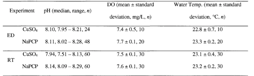
Table 2-1. The pH values, dissolved oxygen (DO) concentrations, and water temperatures o f the CuS04 and NaPCP exposure media.
The pH values were measured for both newly prepared and 12-h exposed water
CuS04 NaPCP
pH 8 . 1 0 8.19
(median) (range=7.89 - 8.27, 154) (range=8.13 - 8.28, «=100)
DO
(mean ± standard deviation, n=20, mg/L) 7.47 ±0.15 7.57 ±0.10
Water Temperature
d u ce d w ith p e rm is sio n of the co p yr ig h t o w n e r. F u rth e r re p ro d u ct io n p ro h ib ite d w ith o u t p e rm is s io n .
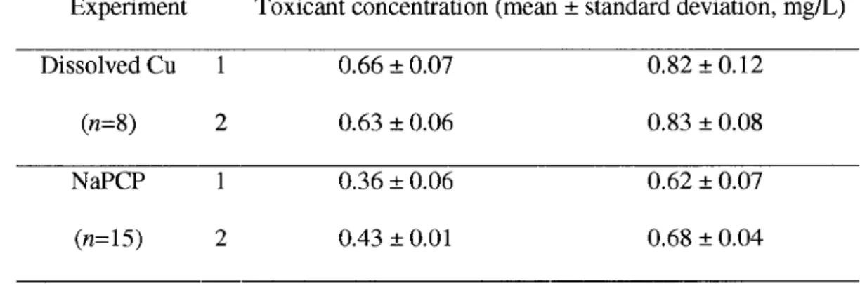
Table 2-2. Measured concentrations o f total dissolved Cu and NaPCP during the 48 h exposures
Toxicant concentrations (mg/L, mean + standard deviation, n = 8)
Experiment # Treatment 1 Treatment 2 Treatment 3 Treatment 4
1 0.19±0.02 0.28+0.03 0.35±0.04 0.53±0.06 Dissolved 2 0.13±0.02 0.22±0.03 0.30±0.04 0.47±0.06 Cu 3 0.13±0.02 0.21±0.03 0.29+0.04 0.45+0.05 1 0.20±0.08 0.36±0.04 0.51±0.03 0.77±0.07 NaPCP 2 0.20+0.05 0.33±0.03 0.51±0.05 0.81±0.03 3 0.19±0.02 0.32+0.06 0.50±0.02 0.79±0.05
d u ce d w ith p e rm is sio n of the co p yr ig h t o w n e r. F u rth e r re p ro d u ct io n p ro h ib ite d w ith o u t p e rm is s io n .
Table 2-3. The Akaike’ s information criterion (AIC ) values and the best-fit accelerated failure time models for Q1SO4 experiments.
A ll the listed coefficients were significantly different from 0 (pcO.OOl)
Experiment
A IC values for each distributiona
M o d e lb
Exponential Log-logistic Log-normal W eibull
General0 315.6 282.0
279.0
287.2 lnTd=3.33-1.39xlnCe+ 0.73xL 1 During f 173.2 123.0 124.6121.6
lnT=3.64-0.58xlnC +0.21xL A fte r g 232.6 231.0230.6
232.2 lnT=2.65-1.99xlnC +1.28xL General 395.2 361.0358.6
369.6 lnT=3.33-0.98xlnC +0.80xL 2 During 2 1 1 . 8 186.4 187.6186.2
lnT=3.37-0.89xlnC +0.40xL A fter 320.2 320.8319.4
322.2 lnT=2.92-1.17xlnC +1.50xL General 421.2 411.2404.6
423.0 lnT=2.64-1.54xlnC +1.24xL 3 During 309.0 280.4275.4
285.6 lnT=2.92-0.90xlnC +0.76xLd u ce d w ith p e rm is sio n of the co p yr ig h t o w n e r. F u rth e r re p ro d u ct io n p ro h ib ite d w ith o u t p e rm is s io n . 33
a The values in bold denote the smallest A IC and the best-fitting distribution,b The best-fit model is indicated by the A IC values,c Model produced by fitting all data, including post exposure m o rtality,d Time-to-death,e Concentration,f Model produced by fitting
d u ce d w ith p e rm is sio n of the co p yr ig h t o w n e r. F u rth e r re p ro d u ct io n p ro h ib ite d w ith o u t p e rm is s io n .
Table 2-4. The Akaike’ s information criterion (AIC) values and the best-fit accelerated failure time models for NaPCP experiments. A ll the listed coefficients were significantly different from 0 (p<0.001)
Experiment
A IC Values for Each D istributiona
M o d e lb
Exponential Log-logistic Log-normal W eibull
Generalc 382.7 359.6
358.6
367.7 lnT“=3 .51--1.11 x lnCe+0.90x L 1 D u rin g f 309.5 248.7 259.7238.3
lnT=3.67-0.56xlnC+0.34xL A fte rg 1 1 2 . 0 110.3108.8
1 1 0 . 6 / h General 343.7 317.7313.2
332.7 lnT=3.18-1.53xlnC+0.83xL 2 During 286.2 224.0218.0
229.1 lnT=3.20-0.99xlnC+0.53xL After72.5
73.5 72.7 73.7 / General 289.0 280.4276.1
285.2 lnT=3.89-1.29xlnC+1.04xL 3 During 240.1 190.7 191.2189.0
lnT=3.79-0.59xlnC+0.32xLd u ce d w ith p e rm is sio n of the co p yr ig h t o w n e r. F u rth e r re p ro d u ct io n p ro h ib ite d w ith o u t p e rm is s io n . 35
aThe values in bold denote the smallest A IC and the best-fitting distribution,b The best-fit model is indicated by the A IC values,c Model produced by fitting all data, including post exposure m orta lity,d Time-to-death,e Concentration,f Model produced by fitting only data from the exposure phase o f the experiments,s Model produced by fitting only the data generated after the exposure ended,h The best-fit models were not listed because the coefficients o f the natural log o f concentration were not significantly different from 0 (<2=0.05)
P ro p o rt io n De ad
Exposure Post Exposure 0.9 0.8 0.7 0.6 0.5 0.4 0.3 0.2 0.1 0
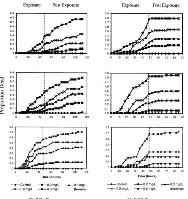
Exposure Post Exposure 0.9 0.8 0.7 0.6 0.5 0.4 0.3 0.2 0.1 0 10 20 30 40 50 60 70 80 90 0.9 0.7 0.5 0.4 0.3 0.2 0 20 40 60 80 100 120 0.8 0.7 0.6 0.5 0.4 0.3 0.2 0.1 0 0 20 40 60 80 100 120 Time (hours) — •— Control — ■— 0.2 mg/L — * — 0.3 mg/L —* — 0.4 mg/L — «— 0.6 mg/L (Nominal) C11SO4 Exposures 0.9 0 .8 0.7 0 .6 0.5 0.4 0.3 0.2 0.1 0.0 0 10 20 30 40 50 60 70 80 90 0.7 0.5 0.4 0.3 0.2 10 20 30 40 '50 60 0 70 80 90 Time (hours) Control — ■— 0.2 mg/L — * — 0.3 mg/L 0.5 mg/L —m— 0.8 mg/L (Nomina!) NaPCP Exposures
Figure 2-1. The cumulative proportions o f amphipods dead through time for the CuSC>4
and NaPCP exposures. The groups o f lines indicate different nominal toxicant
concentrations. (Refer to Table 2-2 for measured toxicant concentrations.) The dashed lines at 48 h separate exposure and post exposure periods.
oc e cn <D
>
o U 1 □ C o n v e n tio n a l L C 5 0 0.9 0.8 B C o m p le te L C 5 0 0.7 0.6 0.5 0.4 0.3 02 0 .1 oExp 1 Exp 2 Exp 3 C11SO4 Exposures 00 E 00 O =5 13 > o U 1 OS □ C o n v e n tio n a l L C 5 0 0.8 □ C o m p le te L C 5 0 0.7 0.6 0.5 0.4 0.3 02 0.1 o Exp1 Exp3 NaPCP Exposures
Figure 2-2. Conventional (during the exposure) and complete (exposure plus post
exposure) LC50 values for the CUSO4 and NaPCP experiments. The error bars indicate
their 95% fiducial limits and Exp 1, 2, and 3 denote the first, second, and third experiment, respectively.
^3 03 0) Q a o ' f i o Q. OUh CU T3 03 O Q G O G o CU o cu 100% 90% 80% 70% 60% 50% 40% 30% 20% 10% 0% 100% 90% 80% 70% 60% 50% 40% 30% 20% t)%
Exp 1 Exp 2 Exp 3
C11SO4 Exposure
□ P redicte d P ro p o rtio n
B P ro p o rtio n including Latent M o rta lity
54% 55% , 50% ____ 5 0 % r - _ 5 0 % '
Exp 1 Exp 2 Exp 3
NaPCP Exposure
Figure 2-3. The predicted proportion dead at the conventional LC50 values and the
proportion dead after including latent mortality for the CUSO4 and NaPCP experiments.
0.5 0.5 10 20 30 0 10 20 30 50 0 40 50 40 00 0.5 0.5 10 50 0 20 30 40 50 0 10 20 30 40 0.5 10 20 0 30 40 50 2 1.5 1 0.5 0 0 10 20 30 40 50 p=0.1 — P=0.3 P=0.5 —---P = 0 .7 ...P=0.9 — • — 48hou rL C 50 Time (h)
C11SO4 Exposures NaPCP Exposures
Figure 2-4. Response contours generated from survival models o f 48 h exposures to
CUSO4 and NaPCP. The lines indicate different proportions dead. The 48 h LC50 values
CHAPTER III. PULSED EXPOSURE: EFFECTS OF PULSE D UR ATIO N AN D RECOVERY TIM E BETWEEN PULSES
A. Introduction
Although most pulsed exposure studies have been conducted on mammals, increasing attention is being paid to effects of pulsed toxicant exposures characteristic o f spills, episodic surface runoff, applications o f agrochemicals, and many industrial discharges. For most o f the time, aquatic organisms are exposed to background levels of toxicants with lethal concentrations being reached periodically. Prediction o f lethal consequences o f pulsed exposure through conventional LC50 methods is often difficult because conventional methods are associated with a fixed duration and constant
concentration, as was discussed in Chapter II. They also do not routinely include latent mortality. For these reasons, they may not be adequate for prediction of pulsed exposure effects for which concentration, duration, and pulse frequency change through time.
Some researchers realize the inadequacy o f the conventional methods and have begun exploring pulsed exposure effects in different ways. A llin and Wilson (2000) investigated the sub-lethal acclimation effect on the 4 d lethal pulsed exposure to
aluminum (Al) with juvenile rainbow trout, Oncorhynchus mykiss. The swimming
behavior, mortality, and hematological changes were compared between the A l
acclimated and naive groups. The results suggested that previous exposure to sub-lethal levels o f A l in the natural environment could be an important factor abating A l impact.
The effects o f pulse frequency and interval among multiple chlorpyrifos exposures on mortality, m obility, and natality o f Daphnia magna were evaluated (Naddy and Klaine 2001). It was suggested that the organism could recover from the previous lethal
chlorpyrifos exposure i f there was adequate time for recovery between exposures. Clark et al. (1986) found that multiple-pulse exposures o f substances were less toxic to
aquatic organisms than continuous exposures o f equal total duration. The reasons may be that some detoxification, repair, or elimination occurring during the non-toxic period can reduce the toxic effects of the earlier exposures (Parsons and Surgeoner 1991) and is dependent on the length o f time between pulses (Wang and Hanson 1985). Reinert et
al. (2 0 0 2) discussed the tools for deciding whether time-varying exposures are relevant
in a particular risk assessment and approaches for laboratory toxicity testing, modeling, and risk characterization. However, most o f these studies either made the predictions semi-quantitatively with statistical method such as conventional analysis o f variance (ANO VA), or did not incorporate duration effectively. Quantitative models that incorporate duration effect are needed to make better predictions.
In addition to exposure concentration and toxicant modes o f action as discussed in Chapter II, other variables such as pulse duration and recovery time between pulses can be important in order to better predict field population fate in pulsed exposures. Pulse duration could affect latent mortality, and recovery time could influence how an organism w ill respond to a subsequent exposure. Low latent mortality and long time for recovery could result in better recovery, and therefore, the effects o f subsequent pulses w ill be less dependent on the previous exposure. To explore these hypotheses, I
Specifically, I asked: (1) is there any effect o f exposure duration on latent mortality, (2) can the complete recovery time (i.e., the time that an organism needs to return to its original level o f toxicant resistance) be predicted, and (3) what is the relationship between recovery time between pulses and mortality during the second pulse. Copper sulfate and NaPCP were used because they have contrasting levels o f latent mortality. To address the first question, H. azteca was exposed to two toxicant concentrations for three durations. The effect o f exposure duration on latent mortality was quantified with survival modeling. For the second and third questions, the amphipods were provided four different recovery times between two pulses o f the same concentration and duration. Time-to-death data collected during the second exposure were modeled, the complete recovery times estimated, and the effect o f recovery time quantified.
B. Methods
1. Effect o f exposure duration on latent mortality
The amphipod culture, maintenance, and general exposure design were similar to those described before. One to two weeks old amphipods were sieved and acclimated in the
RMHRW for 6 d before the exposures began. Experimental concentrations, durations,
and animal sample sizes were found based on preliminary experiments and the test
results o f Chapter II. In the formal experiments, the CUSO4 and NaPCP were dissolved
in RM HRW to make two nominal concentrations for each (dissolved Cu: 0.8 and 1.0 mg/L, NaPCP: 0.4 and 0.6 mg/L). The amphipods were exposed 20, 38, and 61 h to
Q1SO4, and 20, 40, and 60 h to NaPCP. Both newly prepared and exposed water