MONETARY SCIENCE, FISCAL ALCHEMY Eric M. Leeper
Working Paper 16510
http://www.nber.org/papers/w16510
NATIONAL BUREAU OF ECONOMIC RESEARCH 1050 Massachusetts Avenue
Cambridge, MA 02138 October 2010
Prepared for the Federal Reserve Bank of Kansas City's Jackson Hole Symposium, "Macroeconomic Policy: Post-Crisis and Risks Ahead,'' August 26--28, 2010. I thank my discussant, Francesco Giavazzi, and Ralph Bryant, Troy Davig, Jon Faust, Dale Henderson, Maya MacGuineas, Susan Monaco, Chris Sims, Mathias Trabandt, Anders Vredin, Todd Walker, and symposium participants for valuable conversations and comments. The views expressed herein are those of the author and do not necessarily reflect the views of the National Bureau of Economic Research.
NBER working papers are circulated for discussion and comment purposes. They have not been peer-reviewed or been subject to the review by the NBER Board of Directors that accompanies official NBER publications.
© 2010 by Eric M. Leeper. All rights reserved. Short sections of text, not to exceed two paragraphs, may be quoted without explicit permission provided that full credit, including © notice, is given to the source.
NBER Working Paper No. 16510 October 2010
JEL No. E31,E52,E58,E61,E62
ABSTRACT
Monetary policy decisions tend to be based on systematic analysis of alternative policy choices and their associated macroeconomic impacts: this is science. Fiscal policy choices, in contrast, spring from unsystematic speculation, grounded more in politics than economics: this is alchemy. In normal times, fiscal alchemy poses no insurmountable problems for monetary policy because fiscal expectations can be extrapolated from past fiscal behavior. But normal times may be coming to an end: aging populations are causing promised government old-age benefits to grow relentlessly and many governments have no plans for financing the benefits. In this era of fiscal stress, fiscal expectations are unanchored and fiscal alchemy creates unnecessary uncertainty and can undermine the ability of monetary policy to control inflation and influence real economic activity in the usual ways.
Eric M. Leeper Department of Economics 304 Wylie Hall Indiana University Bloomington, IN 47405 and NBER [email protected]
Eric M. Leeper
I
Introduction
Ten years ago Clarida et al. (1999) proclaimed the arrival of “The Science of Monetary Policy.” Although the past few years’ experiences may have raised some questions about the robustness of the science, the paper’s general theme continues to resonate: modern monetary analysis has progressed markedly from the days of monetary metaphors like “removing the punch bowl” and “pushing on a string.” Key elements in the progress include modeling dynamic behavior and expectations, understanding some of the critical economic frictions in the economy, discussing explicitly central banks’ objectives, communicating policy intentions to the public, developing operational rules that characterize good monetary policy, and deriving general principles about optimal monetary policy.
In a surprising twist of fate, the practice of monetary policy marched along side the theory. Central banks around the world have adopted clearly understood objectives—such as inflation targeting and output stabilization—and central bankers espouse and articulate the science in public discussions about managing expectations, the transmission mechanism of monetary policy, and the role of uncertainty in policymaking. Modern monetary research and practical policymaking are united in aiming to make monetary policy scientific.
No analogous transformation has occurred with macro fiscal policy. Although academic research has progressed, policy discussions reflect little of it. In the place of dynamics and expectations are Keynesian hydraulics and multipliers. Instead of clear objectives and rules, there are one-off “reforms” and Blue Ribbon Commissions.
I mark monetary policy’s transition from alchemy to the time when central bankers realized that the question “What are the effects of raising the short-term interest rate by 50
∗October 26, 2010. Indiana University and NBER, 105 Wylie Hall, Bloomington, IN 47405; phone:
(812) 855-9157; [email protected]. Prepared for the Federal Reserve Bank of Kansas City’s Jackson Hole Symposium, “Macroeconomic Policy: Post-Crisis and Risks Ahead,” August 26–28, 2010. I thank my dis-cussant, Francesco Giavazzi, and Ralph Bryant, Troy Davig, Jon Faust, Dale Henderson, Maya MacGuineas, Susan Monaco, Chris Sims, Mathias Trabandt, Anders Vredin, Todd Walker, and symposium participants for valuable conversations and comments.
basis points?” is ill-posed because the answer hinges on the expected path of short rates, among other things.
Fiscal policy will shed its alchemy label when the question “What is the fiscal multi-plier?” is no longer asked and detailed analyses of “unsustainable fiscal policies” are no longer conducted without explicit analysis of expectations and dynamic adjustments. Mul-tipliers depend on the type of spending or tax change, as well as on a host of other factors: expected sources and timing of future fiscal financing, whether the initial change in policy was anticipated or not, and how monetary policy behaves. “Unsustainable policies” can’t happen. When investors believe current policies will last forever, they bid the value of gov-ernment bonds to be consistent with those expectations; in severe cases, that value may be zero. But in economies, like the United States, whose policies are deemed “unsustainable” despite highly valued debt, traders must not believe current policies will persist. The notion of “unsustainable policies” builds in assumptions about future policies that are chronically at odds with bond holders’ beliefs.
The science-alchemy terminology doesn’t mean monetary policy has achieved the scien-tific pinnacle. Neither does it imply that all fiscal analysis is voodoo.1 The terminology is designed to call attention to the generalization that monetary policy tends to employ system-atic analytics, while fiscal policy relies on unsystemsystem-atic speculation. If you explicitly model the things that we know matter—expectations, purposeful behavior, dynamic adjustments, uncertainty—then you are engaged in science. Otherwise, you are doing alchemy.
How is the claim of monetary science sustained? We have known at least since Fried-man (1948) that monetary and fiscal policies are intricately intertwined and their distinct impacts are difficult to disentangle. We also know from work over the past few decades that recalcitrant behavior by one policy authority can easily thwart the other authority’s efforts to achieve its objectives. One major macro policy tool cannot hope to be scientific if the other major tool practices alchemy. Going forward, the sustainability of monetary science may be in jeopardy.
The sharp contrast between the science of monetary policy and the alchemy of fiscal policy is puzzling when viewed from the perspective of a macroeconomist. There are clear parallels between the two macro policy tools. Both can have strong effects on aggregate demand, inflation, and economic activity. Dynamics, expectations, and asset prices play central roles in transmitting the impacts of both policies. Dynamic private behavior creates
1In fact, there is quite a lot of fiscal science being conducted, for example, in the public finance and optimal
fiscal policy fields [for example, Golosov et al. (2006) and Kocherlakota (2010)]. On the more applied side, Bryant et al. (1993) and Bryant and Zhang (1996) are examples of fiscal science that explored the impacts of alternative fiscal rules that ensure policy is sustainable. That science, however, does not seem to have spilled over significantly into macro fiscal policy analyses or into practical fiscal policy evaluation.
time inconsistency problems for both policies. And both are most effective when they are credible and predictable. Fiscal alchemy is all the more puzzling because in many ways it is the more powerful tool. Fiscal policy can also have important supply-side impacts through infrastructure expenditures, spending aimed at human capital accumulation, and taxes that directly affect the after-tax returns to labor and capital. Adjustments to fiscal actions occur over decades, giving fiscal policy long-lasting impacts. Investments in developing the science of fiscal policy are likely to have high social returns.
Responsibility for the application of fiscal alchemy in policymaking falls squarely on governments and legislatures who, for many years, have refused to invest in the intellectual capital that could lead to more economically sound policy decisions. Political leaders much prefer the discretion that alchemy offers over the discipline that science imposes. Resistance of policymakers to adopting rules to guide their fiscal decisions is a key example of this revealed preference. It’s also an odd state of affairs. One would imagine that political leaders who seek to implement good economic policies might welcome the cover that fiscal rules provide.2 It is far easier to tell a constituency that it’s impossible to give them more fiscal goodies because the rules prevent it than it is to explain that doing so is unsound macroeconomic policy. Perhaps it is possible to design institutional reforms that would be good politics, as well as good economics.
I.A Anchoring Fiscal Expectations Monetary and fiscal policies and their
interac-tions is a vast topic that requires an organizing principle. The anchoring of expectainterac-tions is such a principle because it embeds the central tenets of modern economic science: dynamic behavior, purposeful decision making, the roles of information and uncertainty, and the on-going nature of policymaking. Anchoring expectations has become so ingrained in monetary policy that it is something of a mantra; fiscal authorities rarely discuss it.3
In normal times, fiscal alchemy poses no insurmountable problems for central banks. Even if policy institutions do not firmly anchor fiscal expectations, people can use past fiscal behavior to guide their beliefs about the future. But normal times may be nearing their end. The International Monetary Fund calculates that the net present value impact on deficits of aging-related government spending averaged across the advanced G-20 countries is over 400 percent of GDP [International Monetary Fund (2009b)]. Gokhale and Smetters (2007) project that the long-term budget imbalance associated with Social Security and Medicare in the United States this year is over $75 trillion in present value. In the face of fiscal adjustments of these magnitudes, past policy behavior may be a weak reed on which to base
2Maya MacGuineas made this point to me.
3A recent exception—the only one I know—comes, not from a fiscal authority, but from International
expectations.
These numbers portend an extended era of fiscal stress. Problems for central banks become far more pressing during periods of fiscal stress. Combined with fiscal alchemy, fiscal stress threatens to undermine the advances made by monetary policy. Threats do not arise only from insufficient resolve by central bankers to control inflation. Threats arise from unanchored fiscal expectations that can make it difficult or impossible for central banks to control inflation, regardless of the central bankers’ resolve.4
Unanchored fiscal expectations also make it more difficult for consumers and firms to make good economic decisions. Should I be saving more in anticipation of entitlements reform that will reduce my old-age benefits? Should firms build factories on the planned interstate route or will new fiscal austerity measures rescind the authorized infrastructure spending? Will the sunset provisions in the 2001 and 2003 U.S. tax cuts be enforced or will the cuts be extended? Fiscal institutions do not provide the incentives and constraints necessary to induce policymakers to take actions that would reduce this uncertainty. Consequently, the private sector treats future policies probabilistically to hedge against possible outcomes. Hedging retards economic activity and, inevitably, some decisions will turn out to be badex post. Anchoring fiscal expectations is a worthy goal in its own right.
But why should central bankers care whether fiscal expectations are anchored? It turns out that the central bank’s ability to control inflation and influence real activity rests fun-damentally on fiscal behavior and people’s expectations of fiscal behavior. When those expectations center on the appropriate fiscal behavior, the central bank can affect economic activity and inflation in the usual ways. But when fiscal expectations are anchored elsewhere, it’s quite possible that monetary policy can no longer do its job controlling inflation and sta-bilizing real activity. In the coming era of fiscal stress with no credible government plans to confront the growing fiscal strains, unanchored fiscal expectations become a certainty.
Differences between the practices of monetary and fiscal policy are not intrinsic to their respective policy tools. Instead, the contrast is an outgrowth of the different institutional settings that societies have chosen for the two types of macro policies. Many countries have made monetary policy independent, while keeping fiscal policy politicized. There is a fairly clear consensus on the objectives of monetary policy, but none for fiscal policy (besides the minimal requirement that the government be solvent).5 Even “independent” monetary
pol-4In an insightful new paper, Eusepi and Preston (2010) obtain similar results in an environment in which
individuals are learning about the monetary and fiscal policy regimes.
5Leeper (2009) points out that solvency is the one objective fiscal authorities around the world share.
Be-yond that rather minimal goal, fiscal authorities claim a laundry list of inevitably more politicized objectives, including maximizing economic growth, combatting climate change, reducing smoking, raising productivity, strengthening national security, predicting and preventing economic and financial crises, reducing poverty at home and abroad, equalizing income distribution, and building infrastructure. These are all worthy goals,
icy decisions are scrutinized by governments; governments’ fiscal choices are not scrutinized in any organized form (except obliquely through elections and, in s small handful of coun-tries, by independent fiscal policy councils or related agencies). As a consequence of these institutional differences, public discourse about monetary policy is far more sophisticated and helpful to private decision makers than are discussions of fiscal policy.
I.B Policy Analysis is Hard Faust (2005) observes that applied monetary policy
analysis is “hard” in the sense that even the best dynamic models are “grossly deficient” and this condition is not likely to improve dramatically in the near term. Despite their shortcomings, Faust argues that models, appropriately used, can contribute to policymaking. For all the reasons that Faust articulates, plus its complex and political nature, fiscal policy analysis is “harder.” And even though fiscal models are still more deficient and urgently need further development, they nevertheless can be used to highlight and understand elements of fiscal policy that policymakers often do not consider. This paper raises some of these elements and shows how models can help policymakers think about them.
Fiscal complexity stems from several sources. Myriad tax and spending instruments pro-duce a wide range of macroeconomic and distributional effects. Deficit financing intropro-duces issues of debt management—the level at which to stabilize debt, the speed of stabilization, and the maturity structure of the debt. Fiscal changes affect intra- and intertemporal mar-gins, which induce responses in expectations and behavior over time. Those responses can take decades to play out, giving fiscal actions long-lasting impacts. Fiscal initiatives are de-bated at length and individuals continually update and act on their beliefs about future taxes and spending, which creates intricate interactions between fiscal news and private behavior. Finally, fiscal effects also vary with the monetary policy environment, so that studying fiscal policy in isolation may distort our understanding of fiscal effects. I draw on results that my coauthors and I have obtained to illustrate many of these complexities.
Because fiscal actions can have strong distributional consequences, fiscal decisions are intrinsically political. A given fiscal change almost inevitably has winners and losers who feel the effects directly and often can link those effects to a specific policy decision. Democracy demands that these decisions be ground out by the political process, a process that rarely conforms to scientific standards.
Does this mean we must abandon the aim of elevating fiscal analysis to the level to which monetary policy aspires? I sure hope not. But elevating fiscal analysis requires isolating those
but until they are prioritized and checked for internal consistency, they cannot help guide fiscal expectations. This partial list of objectives comes from publications by Australian Treasury (2008), New Zealand Treasury (2003), Government Offices of Sweden (2009), HM Treasury (2009), and U.S. Department of the Treasury (2007).
aspects of fiscal policy that are less political and more amenable to science. Less political aspects of fiscal policy, on which societal and professional consensus may be possible, include: whether a debt target is desirable and what that target should be; how rapidly tax rates and spending should adjust to stabilize debt; circumstances, if any, when changes in the debt target are permissible.
That fiscal policy is “harder” calls for more dynamic modeling, more emphasis on ex-pectations, more attention to information and uncertainty, more effort to confront dynamic political economy models with data, more professional scrutiny, and more focus on institu-tional design. In a phrase, more science. It is ironic that fiscal policy receives less of all these things than does monetary policy.
I.C What the Paper Does The next section presents three topical examples where
fiscal alchemy is finding a voice in current policy debates. Section III steps back to the abstract world to explain how monetary and fiscal policy jointly stabilize inflation and the value of government debt. That section establishes two general principles. First, inherent symmetry in the two macro policies implies that either policy can stabilize inflation and aggregate demand, so long as the other policy maintains the value of debt. Second, if monetary policy is to successfully control inflation and stabilize the real economy, then fiscal policy must free monetary policy to pursue those objectives. This imposes restrictions on fiscal behavior that may be difficult to achieve in times of fiscal stress. Section IV turns to the literature on fiscal multipliers, which is precisely the morass that we would expect alchemy to produce. The section reports results that coauthors and I have obtained that show how sensitive fiscal multipliers are to aspects of the fiscal-monetary policy environment. Unfortunately, I cannot claim that the research provides all the right answers, but it does ask some of the right questions and it aims to address them in ways consistent with fiscal science.
Section Vpresents long-term fiscal projections to explain why many advanced economies are heading into an era of fiscal stress. It defines the “fiscal limit,” the point at which, for economic or political reasons, fiscal policy can no longer adjust to stabilize debt, and explores some surprising implications that arise when an economy is staring at the prospect of a fiscal limit. For example, information that shifts expected paths of spending or taxation can have important effects on aggregate demand today, well before the fiscal changes occur. Research discussed in section VI describes one constructive route to modeling economic behavior in an era of fiscal stress. That route posits what people might believe about how future policies may adjust in response to fiscal stress and derives the macroeconomic consequences of those adjustments. SectionVIIsuggests some roles that central banks and their leaders could play
in the era of fiscal stress. Key among these is for central bankers to break the taboo against saying anything substantive about fiscal policy and, instead, to talk precisely and forcefully about how unresolved fiscal stresses can make it difficult or impossible for monetary policy to do its job.
Skeptics might say that fiscal policy is intrinsically political and efforts to make it more scientific are pie in the sky. To those skeptics I address the final section. There I offer some thoughts about separating fiscal policy into its micro and its macro components. Micro components involve distributional issues and rightfully belong in the political realm. But I try to identify some macro aspects that are largely technical matters that lend themselves to fiscal science. Economists may be able to coalesce on the macro fiscal issues, even while the micro issues remain contentious.
II
Fiscal Alchemy in Action: Recent Examples
Fresh examples of alchemy in fiscal policymaking appear in the news regularly [for example, Hilsenrath (2010)]. In this section I highlight three prominent examples of fiscal alchemy in policymaking. I select these examples because they are timely and they are at the forefront of important policy debates. Far more egregious but less current examples abound.
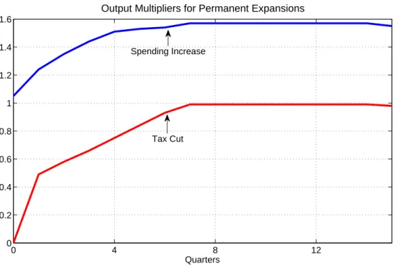
Fiscal multipliers: A report authored by Romer and Bernstein (2009) provided impor-tant support for the Obama administration’s effort to stimulate the U.S. economy through the $787 billion American Recovery and Reinvestment Act of 2009. Fiscal multipliers as-sociated with government spending increases and tax cuts, which appear in the report, are reproduced in figure 1. Government spending packs more punch than taxes, as shown in the figure. The report also provides detailed estimates of the number and types of jobs that a stimulus package would create.
Graphics like figure 1, and hundreds of others that pepper the empirical fiscal policy literature, leave the reader wanting to know more. What are the economic mechanisms through which the stimulus would add to employment? How will “permanent” changes in spending or taxes be supported by adjustments in other fiscal instruments in the future? How might alternative adjustments affect the multipliers? Are the fiscal changes anticipated or unanticipated? What happens to the output multiplier in the medium to long run, beyond the four-year horizon reported? Sources for the multiplier numbers are given as “a leading private forecasting firm and the Federal Reserve’s FRB/US model,” which are not in the public domain and cannot be professionally scrutinized. How would a researcher reproduce the multipliers that Romer and Bernstein (2009) report? Overall, the report’s rationale for the stimulus package do not rise to the scientific standards to which monetary policy analyses
aspire.6 0 4 8 12 0 0.2 0.4 0.6 0.8 1 1.2 1.4 1.6
Output Multipliers for Permanent Expansions
Quarters Spending Increase
Tax Cut
Figure 1: Output multipliers for a permanent increase in government spending or a perma-nent decrease in taxes, as reported in Romer and Bernstein (2009).
Fiscal retrenchments: Defenders of fiscal retrenchment often argue that
retrench-ment can actually be expansionary. Research has found some evidence that under some circumstances fiscal consolidations have had beneficial economic effects, or at least have not produced declines in economic activity [Giavazzi and Pagano (1990), Bertola and Drazen (1993), Alesina and Ardagna (1998)]. Much of that evidence comes from case studies that examine a single country that undertakes a sizeable, isolated fiscal consolidation. There is no evidence that if many countries—say, much of Europe—undertake fiscal austerity measures simultaneously, then economic activity will improve.
To be sure, fiscal multipliers depend on the state of the economy and can change over time. But can they changesignin a little over a year? Does any model exist to show that 18 months ago it made sense for the United Kingdom to expand fiscal policy, while now it makes sense to implement the recently announced 25 percent nearly across-the-board budget cuts? As Alesina and Ardagna (1998) make clear, an intricate set of conditions needs to be in place
6To be fair, U.S. fiscal actions are rarely supported by research that meets generally accepted standards.
U.S. Department of the Treasury (1984) followed the Reagan tax cuts and argued that deficits had no effects on interest rates. The Bush tax cuts in 2001 initially were justified by little more than the observation that the federal budget surpluses were “your money” along with the claim that lower marginal tax rates would stimulate economic activity.
for consolidations to be expansionary—“the tightening must be sizeable and occur after a period of stress when the budget is quickly deteriorating and public debt is building up.. . . To be long lasting, it must include cuts in public employment, transfers and government wages. To be politically possible, such a policy must be supported by trade unions.” Those authors also point out that several issues are “not settled,” but are critical to determining which fiscal consolidations will contract the economy and which will expand it.
Fiscal flip-flops are being justified in the name of credibility. Countries feel the need to contract fiscal policy in the midst of a weak recovery because fiscal institutions provide no other mechanism by which fiscal decision makers can establish the longer run soundness of their policies; as a consequence, with fiscal expectations unanchored in general, politi-cal leaders speculate that bold contractionary actions will prove their mettle and, in some unspecified way, improve economic conditions. Paul Volcker was forced into an analogous difficult situation in the early 1980s to demonstrate the Fed’s bona fides as an inflation fighter. But at that time there was no pretense that tight monetary policy would not hurt the economy. Current fiscal flip-flops are about solving today’s problem; but credibility is inherently a long-run trait that can be established only by changing the fiscal institutions on which fiscal expectations are based. One-time fiscal consolidations most often do not morph into permanent fiscal reforms. Many countries institutionalized monetary policy re-forms by adopting inflation targeting. There is, at best, ambiguous scientific support for the coordinated fiscal contraction that is taking place.
Long-term fiscal projections: In some countries a fiscal agency issues regular reports on its country’s long-term fiscal situation. The reported paths of endogenous fiscal vari-ables, like government debt, typically do not emerge as implications of an economic model: given a set of assumptions, debt paths pop out from an accounting relation that equates current debt to past debt plus current deficits. When the resulting paths show debt grow-ing exponentially at a rate faster than the economy, the agency declares that fiscal policy is on an “unsustainable path.” Logically, though, unsustainable policies cannot occur, so the agency’s projections cannot happen. Reporting things that cannot happen cannot help people make economic decisions.
The Congressional Budget Office’s (2009; 2010c) long-term projections in 2009 and 2010 make clear how unhelpful government macro fiscal analyses can be. This year’s baseline projection differs dramatically from 2009, with debt at almost 300 percent of GDP at the end of the projection period in the 2009 report, but at just over 100 percent of GDP in the 2010 exercise [figure2]. That’s the rosy scenario. The alternative projections build in policy changes the CBO deems likely to occur—for example, curtailing the reach of the Alternative Minimum Tax and extending most of the provisions of the 2001 and 2003 tax cuts—and
have debt exceeding 700 percent and 900 percent in the 2009 and 2010 projections. 17900 1810 1830 1850 1870 1890 1910 1930 1950 1970 1990 2010 2030 2050 2070 2084 100 200 300 400 500 600 700 800 900 Percentage of GDP Baseline Scenario 2010 Baseline Scenario 2009 Alternative Scenario 2009 Alternative Scenario 2010
Figure 2: Projections of U.S. federal government debt as a percentage of GDP from Con-gressional Budget Office (2009, 2010c).
Figure 2 is amenable to alternative interpretations. (1) According to the baseline, the long-term U.S. fiscal position improved sharply over the past year, in large part because of substantial cost savings from the recent health reform bills, so the need for serious fiscal reform is less pressing.7 (2) The alternative projection, in contrast, suggests that the fiscal position has deteriorated further, with the debt-GDP ratio rising to almost 1000 percent at the end of the projection period. (3) Viewing the baseline and alternative as two points on a probability distribution, the dispersion in the distribution has increased dramatically, suggesting a significant increase in uncertainty about future fiscal actions. (4) Because the
7This is the interpretation adopted by some economic bloggers. See, for example,
http://www.angrybearblog.com/2010/06/cbo-releases-long-term-budget-outlook.html, which refers to
“deficit hysterics” and then comments: “Interestingly if we examine the above two figures we see that ’Extended baseline’ which essentially means ’Current law’ shows the deficit vanishing by 2014 and Debt Held by the Public stabilizing through 2035. Making some of the ‘If this goes on the sky will fall!’ rhetoric around Obama policy a little overstated, just as with Social Security a plan of ‘Nothing’ getting oddly some pretty good projected results.”
projections are accounting exercises and do not come from any coherent economic model, they are not economic forecasts and it’s foolhardy to try to draw meaningful economic inferences from them. This is confusing economics. Because the baseline is a scenario that nobody believes will happen and the alternative is an outcome that everyone know cannot
happen, the CBO’s projections do little to help people form expectations over future fiscal policies and they do not constitute science.8
As the introduction suggests, the source of the CBO’s less-than-informative long-term projections is the tightly circumscribed mandate that the U.S. Congress imposes on the CBO. By law the CBO must construct projections assuming that current law remains in effect. Baseline and alternative scenarios are two interpretations the CBO ascribes to “current law.” But when “current law” is unsustainable, projections conditioned on it have little economic content. It is important to acknowledge, though, that the CBO is simply a conduit for Congress’ alchemy.
III
Monetary-Fiscal Interactions in Normal Times
Most macroeconomists were raised on the belief that inflation is determined by monetary policy, especially in the long run. Full stop. Sure, especially egregious fiscal policy or wartime finance might force the central bank to print money, accumulate government bonds, and generate inflation. But even in this instance, the overall price level is being determined by the interaction of money supply and money demand: inflation is a monetary phenomenon. New Keynesian models couch monetary policy in terms of controlling a nominal interest rate, rather than high-powered money, but otherwise new Keynesian and old monetarist are close cousins in terms of thinking about how inflation gets determined.
Central bankers need a broader perspective on price level determination—to at least understand and acknowledge that there is another channel through which inflation can be determined. The broader perspective is important because the new Keynesian/old mone-tarist view implicitly embeds adirty little secret: for monetary policy to successfully control inflation, fiscal policy must behave in a particular, circumscribed manner.9 When fiscal policy fails to behave appropriately—as it may during economic crises or periods of fiscal
8In fact, these long-term projections build in a variety of assumptions about the economy’s evolution over
the projection period: within a few years, inflation is constant at 2.5 percent, real interest rates at 3 percent,
unemployment at 5 percent, and so on. Taken on face value, the economy chugs along just fine even as
government debt explodes. The CBO reports then lapse into wordy bits about the dire consequences of rapid growth in government debt. These wordy bits are speculative and not derived from some economic model employed by the CBO. Wordy speculation about the possibility and likely consequences of a fiscal crisis in the United States appears in a special CBO report, Congressional Budget Office (2010b).
9Although Friedman (1960) is explicit about this necessity in hisA Program for Monetary Stability, as is
stress—then inflation can get determined in a very different, unconventional, way. In this section I focus on inflation, but this should be construed more broadly as aggregate demand. In a more detailed model, some inflation effects would manifest as effects on output and employment.
In the simple model sketched below, macro policies have only two objectives: determine the inflation rate and stabilize government debt. The conventional assignment problem gives monetary policy responsibility for providing a nominal anchor—inflation—and fiscal policy the role of providing a real anchor—the real value of government debt. Because fiscal policy is assigned to stabilize debt, monetary policy is free to target inflation. As a logical matter, however, the assignments can be reversed: fiscal policy can determine inflation, while monetary policy prevents debt from becoming unstable. This alternative assignment may be necessary if, for political or economic reasons, fiscal policy simply cannot make the adjustments needed to stabilize debt.
III.A Fixing Ideas with a Model To fix ideas about how monetary and fiscal policies
must interact to determine inflation and stabilize government debt, I draw on results from an extremely simple model that captures many of the important features of the models used to study price-level determination [Leeper (1991), Sims (1994), Woodford (1995)]. The model abstracts from “money,” but this does not mean monetary policy cannot have powerful effects through changes in the nominal interest rate. The abstraction merely reflects the fact that seigniorage is a trivial fraction of total revenues in most advanced countries, so for simplicity I set it to zero. Appendix A presents the formal model. Here I bring out key features of the model and of policy behavior and then jump to their implications.
Expectations enter the model in two ways. First, individuals’ savings decisions ensure that the expected returns on real and nominal assets are equalized. This behavior produces a Fisher relation that connects the nominal interest rate on short-term government bonds to the real interest rate and the expected inflation rate
Rt=rt+Etπt+1 (1)
whereR and r are the nominal and real interest rates and Etπt+1 denotes the expected rate of inflation between today and tomorrow.
A second role for expectations comes from individuals’ consumption decisions, which depend on their wealth. Wealth is composed of the value of current asset holdings plus the expected present value of after-tax labor income. Because monetary and fiscal policies influence expectations of both inflation and taxes, individuals will track policy behavior and use that information to help them form those expectations.
Policy behavior is stylized. Government transfer payments to individuals, denoted by z, evolve autonomously. Behavior of the monetary and tax authorities is purposeful. Monetary policy adjusts the short-term nominal interest rate to target inflation atπ∗, with the degree to which policy leans against inflationary winds given by α
Rt=R∗+α(πt−π∗) (2)
Tax policy targets the real value of government debt (or the debt-output ratio) at b∗ by adjusting taxes in response to the state of government debt with the strength of adjustment determined by γ τt=τ∗ +γ Bt−1 Pt−1 −b ∗ (3)
where B is the nominal value of bonds outstanding and B/P is their real value. R∗ and τ∗ are the instrument settings when inflation and debt are on target.
A final piece of this stylized model is the government’s budget constraint, which equates sources of financing—new bond sales and taxes—to uses—transfer payments and principal plus interest on old bonds
Bt
Pt +τt=zt+
Rt−1Bt−1
Pt (4)
Policy behavior is not completely described until we take a stand on the sizes of the two critical policy parameters, α and γ, which describe how strongly policies react to deviations of variables from their targets. It turns out that there are two different combinations of monetary and fiscal policies that can jointly stabilize both the inflation rate and the value of debt. I label those two ways Regime M and Regime F.10
III.A.i Regime M The first policy mix is familiar to most macroeconomists, accords
well with how many central bankers perceive their behavior, and frequently applies to policy behavior in normal times. I label this “Regime M” because it is consistent with the mon-etarist aphorism “inflation is always and everywhere a monetary phenomenon.” Regime M emerges when the central bank aggressively targets inflation by raising the nominal interest rate sharply in response to incipient inflation. This is Taylor’s (1993) principle and is called “active” monetary policy, following the terminology in Leeper (1991). An active authority is free to pursue its objectives in an unconstrained manner. Naturally, if monetary policy is attending to inflation targeting, then fiscal policy must handle debt targeting by adjusting taxes enough to achieve the debt target. When an increase in debt induces taxes to rise by
10The present model is too simple to provide any insights into which combination of policies is “better”;
more than the real interest rate, future taxes are assured to be sufficient both to service the new debt and to eventually retire debt back to target. This is called “passive” fiscal policy. Many variants of this regime exist in the literature. Older models of monetary policy typically couched policy behavior in terms of setting high-powered money, rather than the nominal interest rate. But the maintained assumption that fiscal policy is committed to targeting the real value of government debt is identical, although the assumption frequently is not explicitly articulated.
The equilibrium in this regime implies that inflation always equals its target, as does expected inflation
πt=π∗ (5)
Tax policy stabilizes debt gradually by raising taxes enough to cover interest payments and to retire a bit of the principal each period. For example, if transfers rise today, they are initially financed entirely through new sales of government bonds. Those new bonds, though, raise expected and actual future taxes through the tax rule in equation (3).
In this simple model the only source of uncertainty is random transfers. It appears as though monetary policy single-handedly keeps inflation on target by preventing shocks to transfers, which in principle affect household wealth and demand for goods, from transmit-ting into the inflation rate. To understand how monetary policy achieves this, we need to revisit monetary policy’s dirty little secret: fiscal policy is ensuring that higher debt-financed transfers today create the expectation of higher taxes in the future. Those higher taxes are just sufficient to gradually retire debt back to target, eliminating the wealth effect of the higher transfers and relieving the pressure on inflation to rise.
Another perspective on the fiscal financing requirements when monetary policy is tar-geting inflation emerges from a ubiquitous equilibrium condition. In any dynamic model with rational agents, government debt derives its value from its anticipated backing. In this model, that anticipated backing comes from tax revenues net of transfer payments, τt−zt. The value of government debt can be obtained by imposing equilibrium on the government’s flow constraint, and taking conditional expectations to arrive at
Bt
Pt = expected present value of primary surpluses from t+ 1 onward (IEC) This intertemporal equilibrium condition, (IEC), provides perspective on the crux of passive tax policy. Because monetary policy nails down the price level and the expected path of transfers, the z’s, is being set independently of both monetary and tax policies, any increase in transfers att, which is financed by new nominal bond sales,Bt,mustgenerate an expectation that taxes will rise in the future by exactly enough to support the higher value
of debt.
Although here only transfers can change debt, passive tax policy implies that this pattern of fiscal adjustment must occur regardless of the reason that debt increases: economic down-turns that automatically reduce taxes and raise transfers, changes in household portfolio behavior, changes in government spending, or central bank open-market operations.
To expand on the last example, we could modify this model to include money and imagine that the central bank decides to tighten monetary policy at tby conducting an open-market sale of bonds. If monetary policy is active, then the monetary contraction both raises Bt— the dollar value of bonds held by households—and it lowers Pt; real debt rises. This can be an equilibrium only if fiscal policy is expected to support it by passively raising future tax revenues.11 That is, given active monetary policy, (IEC) imposes restrictions on the class of tax policies required for equilibrium; those policies are labeled “passive” because the tax authority has limited discretion in choosing policy. A passive authority is constrained both by the inflation process that the active authority determines and by the optimal choices of private economic agents. Refusal by tax policy to adjust appropriately undermines the ability of open-market operations to affect inflation in the conventional manner.12 Evidently, predictable and reliable fiscal adjustments—in a phrase, anchored fiscal expectations—are essential for monetary policy to succeed in targeting inflation.
Although conventional, this regime is not the only mechanism by which monetary and fiscal policy can jointly deliver an equilibrium with stable inflation and debt. We turn now to the other case, which becomes increasingly pertinent in times of fiscal stress.
III.A.ii Regime F Passive tax behavior that occurs in Regime M is a stringent
re-quirement: the fiscal authority must be willing and able to raise taxes or otherwise adjust surpluses in the face of rising government debt. For a variety of reasons, this does not always happen. Sometimes political factors—such as the electorate’s resistance to higher taxes— prevent taxes from rising as needed to stabilize debt. Some countries simply do not have the fiscal infrastructure in place to generate the necessary tax revenues. Others might be at or near the peaks of their Laffer curves, constraining their ability to raise revenues. In these cases, tax policy is active. Analogously, there are also periods when the concerns of monetary policy move away from inflation stabilization and toward other matters, such as output or financial stabilization [see, for example, Board of Governors of the Federal Reserve System (2009) or Bank of England (2009)]. These are periods in which monetary policy
11Higher future taxes also eliminate any wealth effect arising from the higher level of debt in agents’
portfolios, reinforcing the contractionary effects of the open-market sale.
12This is an application of the general insight contained in Wallace (1981). Sargent and Wallace’s
“Un-pleasant Monetarist Arithmetic” (1981) outcome emerges because the tax authority refuses to respond “ap-propriately,” forcing monetary policy in the future to abandon its inflation target.
is no longer active, instead adjusting the nominal interest rate only weakly in response to inflation. The global recession and financial crisis of 2008-2010 is a striking case when central banks’ concerns shifted away from inflation. Then monetary policy is passive.
We focus on a particular policy mix that yields clean economic interpretations: the nominal interest rate is set independently of inflation,α = 0 and the nominal rate is pegged at R∗, and taxes are set independently of debt, γ = 0 and taxes are constant at τ∗. These policy specifications might seem extreme and special, but the qualitative points that emerge generalize to other specifications of passive monetary/active tax policies.
One result pops out immediately. Applying the pegged nominal interest rate policy to the Fisher relation, (1), yields
Etπt+1 =R∗−rt (6)
Since we are assuming that the real interest rate is independent of monetary policy—a strong and unrealistic assumption in practice—expected inflation is anchored on the inflation target, an outcome that is perfectly consistent with one aim of inflation-targeting central banks.13 It turns out, however, that another aim of inflation targeters—stabilization of actual inflation— which can be achieved by active monetary/passive fiscal policy, is no longer attainable.
The intertemporal equilibrium condition, (IEC), can be written in a more suggestive manner as
R∗B
t−1
Pt = expected present value of primary surpluses from t onward (IEC–2) At timet, the numerator of this expression,R∗Bt−1, is already determined by past debt and the pegged interest rate and represents the nominal value of household wealth carried into the current period. The right side is the expected present value of autonomously set primary fiscal surpluses from dateton, which reduces to a fixed number in each date. This expression reveals how the price level is determined each period: it must adjust to set the market value of debt equal to expected discounted surpluses. Regime F leads to a sharp dichotomy between the roles of monetary and fiscal policy in price-level determination: monetary policy alone appears to determine expected inflation by choosing the level at which to peg the nominal interest rate,R∗, while conditional on that choice, fiscal variables appear to determineactual
inflation.
Some economists have found this equilibrium to be peculiar in some way. Although it may not describe most economies in normal times, it is not so strange. To understand the nature of this equilibrium, we need to delve into the underlying economic behavior. This is
13As I show in sectionVI, when the real interest rate is endogenous, fiscal stress can undermine the central
an environment in which changes in debt donotelicit any changes in expected taxes, unlike in Regime M. First consider a one-off increase in current transfer payments, zt, financed by new debt issuance, Bt. This reduces the right side of (IEC–2). With no offsetting increase in current or expected tax obligations, at the initial price level households feel wealthier and they try to shift up their consumption paths. Higher demand for goods drives up the price level, and continues to do so until the wealth effect dissipates and households are content with their initial consumption plan when the two sides of (IEC–2) are equalized.
Now imagine that at time t households receive news of higher transfers in the future. There is no change in nominal debt at t, but there is still an increase in household wealth at initial prices. Through the same mechanism, Pt must rise to revalue current debt to be consistent with the new lower expected path of transfers: the value of debt falls in line with the lower expected present value of surpluses.
Cochrane (2010) offers another interpretation of the equilibrium in which “aggregate demand” is the mirror image of demand for government debt. An expectation that transfers will rise in the future reduces the household’s assessment of the value of the government debt they hold. Households can shed debt only by converting it into demand for consumption goods; hence, the increase in aggregate demand that leads to higher prices.
Expression (IEC–2) indicates that in this policy regime the impacts of monetary policy change dramatically. When the central bank chooses a higher rate at which to peg the nominal interest rate, with no expected change in surpluses, the effect is to raise the price level next period. This echoes Sargent and Wallace (1981), but the economic mechanism and the associated policy behavior are different. In the current policy mix, a higher nominal interest rate raises the interest payments the household receives on the government bonds it holds. Higher nominal interest receipts, with no higher anticipated taxes, raise household wealth and trigger the same adjustments as above. In this sense, as in Sargent and Wallace, monetary policy has lost control of inflation.14
Regime F emphasizes that expectations about fiscal policy can have important effects on aggregate demand and inflation today. For example, in (IEC–2) news of a future tax cut makes forward-looking agents feel wealthier, inducing them to shift up their demand for goods today and in the future. That higher demand translates into higher current inflation. But all these adjustments begin before the tax cut takes place. Current and past budget deficits may contain little, in any, information about fiscal effects on the economy.
14One-period debt implies that ifR∗ rises att, the inflation rate rises att+ 1. With long-term debt, the
inflation increase is delayed and, as Sims (2010) shows, monetary policy retains its ability to raise nominal rates and reduce inflation in the short run. See also Cochrane (2001).
III.B Generalizing Policy Behavior Regimes M and F above maintain the con-ventional assumption that policy rules do not change over time, so the rule in place today determines expected future policy behavior. Of course, rules can and do change. The pos-sibility that future policy rules may differ from current rules can have a profound effect on expectations and on the resulting equilibrium. For example, Davig and Leeper (2007) show that if monetary policy fluctuates between being active and passive, then a wider range of equilibrium outcomes are possible than under Regime M (even though fiscal behavior is perpetually passive), including ones in which temporarily passive monetary policy behavior amplifies volatility in the macro economy even when monetary policy is active.
If both monetary and fiscal rules fluctuate in a way that shifts the economy between regimes, say between Regimes M and F, then fiscal disturbances always affect inflation— just as they do if Regime F were in place forever—even if monetary policy is currently active. This idea is explored in Davig and Leeper (2006, 2010b) and Chung et al. (2007). Two key points come from this reasoning. First, the effects of both monetary and fiscal policy can vary over time, depending on the prevailing mix of monetary and fiscal policies, how long the mix is expected to prevail, and the mix of policies expected in the future.
Second, the unusual fiscal impacts on inflation that come from Regime F will be larger the more time the economy is expected to spend in Regime F now and in the future. These points underscore the central role of expectations in transmitting fiscal policy to the macro economy.
Once policy behavior is generalized to allow for changes in regime, surprising results emerge because in forward-looking models like those commonly employed at central banks, beliefs about policies in the long run anchor expectations and determine the nature of the equilibrium. If policy rules can fluctuate, then economic agents’ expectations will depend on both current and future rules, weighted by the probabilities of the rules. When agents believe that at times fiscal policy will not respond systematically to stabilize debt, then the properties of Regime F spill over to Regime M and monetary policy’s ability to control inflation will be curtailed.
Heading into an era of fiscal stress, as many advanced economies are, it may be reasonable for individuals to ascribe some probability to a future fiscal regime in which fiscal policy is no longer able or willing to target government debt. And the longer that governments delay making the fiscal reforms that will anchor expectations on the fiscal behavior in Regime M, the more likely it is that central banks will be unable to control inflation.
IV
Fiscal Multiplier Morass
Fiscal multipliers are extraordinarily complex creatures. Little professional consensus exists on their magnitudes, in part because it is difficult to perform the same thought experiment across data sets, econometric techniques, and economic models. There are two significant branches of work on fiscal multipliers. One branch, strongly data driven, is represented in recent work by the research of Blanchard and Perotti (2002), Perotti (2007), Mountford and Uhlig (2009), and Romer and Romer (2010).15 A second branch employs fully specified optimizing models—either estimated or calibrated—and is exemplified by Christiano et al. (2009), Cogan et al. (2009), Traum and Yang (2009), Coenen et al. (2010), Davig and Leeper (2010b), Leeper et al. (2010), and Uhlig (2010).
One clear message emerges from this vast literature: estimates of multipliers are all over the map, providing empirical support for virtually any policy conclusion. The diversity of findings, often based onthe same U.S. time series data, highlights the difficulties in obtaining reliable estimates of fiscal effects and points to the need for systematic analyses that confront fiscal policy’s complexities. Remarkably, Coenen et al. (2010) and Cogan et al. (2009) are intended as meta-studies designed to examine the size of fiscal multipliers across a wide range of dynamic optimizing models, yet they arrive at diametrically opposed conclusions. Coenen et al. (2010) finds substantial economic stimulus from government spending increases in the short and medium run, while Cogan et al. (2009) argue that even in the short run government spending is not efficacious. To date, no effort has been made to reconcile the divergent findings from the two groups of respected economists.
As scientists, we know that a wide range of factors influence the macroeconomic impacts of fiscal actions. When these factors are inadequately accounted for, we would expect the inconclusive conclusions that come from alchemy. Of course, even if research economists were to converge on a consensus about the size of various multipliers based on historical data, going forward it is dicey to apply those findings to practical policymaking in an era of fiscal stress when future fiscal adjustments are anyone’s guess.
Much of my work with coauthors attempts to understand whether the forward-looking issues we emphasize can help to sort through the multiplier morass. Because the work is at an early stage, I cannot say with confidence what the multipliers are. But our work does show that dynamic behavior and expectations formation matter a great deal for understanding how fiscal policy affects the macro economy.
15But see the important work of Caldara and Kamps (2010), which carefully examines whether this
IV.A Fiscal Complexities Fiscal effects are complex for all the reasons that monetary effects are, plus some. Whereas monetary policy normally has a single primary instrument— the short-term nominal interest rate—fiscal policy has many types of spending and taxes and each instrument has its distinct impacts.16 But multiple instruments is not the most impor-tant source of fiscal complexity. Fiscal multipliers also depend on the expected sources— taxes, spending, transfers—and timing—soon or in the distant future—of fiscal financing. Alternative fiscal financing schemes change the future intertemporal margins facing decision makers and can also have important effects on wealth; these two channels can dramatically alter the dynamics of fiscal multipliers, including changing their signs over time.
I illustrate these points with results from a recent paper. Leeper et al. (2010) fit post-war U.S. time series to a conventional neo-classical growth model, extended to include substan-tial fiscal detail: government purchases and transfers and proportional taxes levied against capital and labor income and against consumption expenditures. Fiscal behavior follows simple rules that allow each instrument to respond contemporaneously to output, reflecting automatic stabilizers, and to the lagged debt-GDP ratio. Each instrument also contains a component that evolves autonomously.
Neo-classical growth models cannot produce large multipliers for changes in unproductive government spending, a fact that is well-documented [Monacelli and Perotti (2008)], so the results I present are not intended as definitive measures of “the multiplier.” I seek to highlight how the dynamic patterns of estimated government spending multipliers vary systematically with alternative fiscal financing schemes, a feature that will survive across other dynamic models. The results put a sharp point on the difference between fiscal science, which acknowledges and grapples with these complexities, and fiscal alchemy, which sweeps them under the rug.
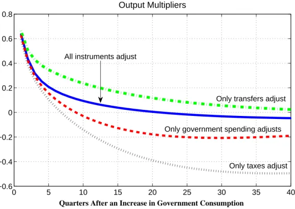
Figure3reports over a 10-year horizon the output multipliers associated with a persistent but transitory increase in government consumption. The figure shows the paths of multipliers under four financing schemes: “All instruments adjust” is the best-fitting model in which all instruments except consumption taxes respond to stabilize government debt; the remaining three paths are counterfactuals in which only a single type of instrument adjusts to finance the increase in government consumption. Short-run multipliers are nearly identical across financing schemes, but within a year of the initial increase in spending, important differences appear. Largest and most persistent positive multipliers emerge when higher spending is financed by lower lump-sum transfers. When higher spending brings forth lower future spending, the multiplier turns negative in about two years and remains negative even 10 years
16Although recent unusual central bank operations make clear that in non-normal times monetary policy
out. The sharpest difference occurs when capital and labor tax rates rise to finance spending, with the multiplier turning negative in six quarters and remaining strongly negative.17
0 5 10 15 20 25 30 35 40 −0.6 −0.4 −0.2 0 0.2 0.4 0.6 0.8 Output Multipliers
Quarters After an Increase in Government Consumption
All instruments adjust
Only taxes adjust Only government spending adjusts
Only transfers adjust
Figure 3: Output multipliers estimated in a neo-classical growth model using post-war U.S. data, as reported in Leeper et al. (2010). Various counterfactual exercises.
The thought experiment underlying figure 3 is controlled in the sense that the only dif-ference across the multiplier paths is the policy rules in place, which determine the sources of future fiscal adjustments and the model agents’ expectations of future policies. Evidently, those expectations are of central importance to determining the dynamic impacts of govern-ment spending. Statistically, the “All instrugovern-ments adjust” path is probably the best guess of the multipliers associated with an exogenous increase in spending, but because in practice fiscal authorities do not follow well-understood rules, any of the adjustments depicted is possible and the values of multipliers, particularly at longer horizons, should be treated as
17Multipliers are present-value multipliers, computed for horizonkas
Present-Value Multiplier(k) = Etkj=0ji=0Rt−+1i ΔYt+j Etkj=0ji=0R−t+1i ΔGt+j
where Y andGare real GDP and real government consumption andR is the model-derived discount rate.
Often the k-period multiplier is calculated as ΔYk/ΔG0, where ΔG0 is the initial change in spending. This textbook-style multiplier, however, is inadequate when changes in government spending generate dynamics in both spending and output.
highly uncertain.
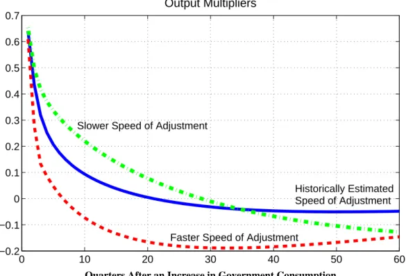
Timing of fiscal adjustments can also be important for determining the size of multipliers. Postponing adjustments pushes changes in taxes and spending into the future and rational economic agents discount distant changes more heavily than near-term changes. Within a week of signing the American Recovery and Reinvestment Act of 2009 (ARRA) into law, President Obama pledged to cut the fiscal deficit in half by 2013 [Calmes (2009)], a promise that would accelerate the adjustment to rising debt. Figure 4 uses the same neo-classical model to show how changes in the speed of adjustment of policy instruments affect the path of the government spending multiplier. Larger multipliers come from slower adjustments, while faster adjustments can reverse the positive output effects rapidly. Again, fiscal expectations are driving the differences.
0 10 20 30 40 50 60 −0.2 −0.1 0 0.1 0.2 0.3 0.4 0.5 0.6 0.7 Output Multipliers
Quarters After an Increase in Government Consumption
Slower Speed of Adjustment
Faster Speed of Adjustment
Historically Estimated Speed of Adjustment
Figure 4: Output multipliers estimated in a neo-classical growth model using post-war U.S. data, as reported in Leeper et al. (2010). Various counterfactual exercises in which all fiscal instruments adjust to stabilize debt.
Fiscal dynamics can take decades to play out. With an estimated dynamic model of fiscal policy in hand, one can ask, “How long does it take for long-run fiscal balance to be restored after various fiscal actions?” Leeper et al. (2010) estimate that fiscal adjustments in the United States have been extremely gradual, taking three or more decades. This is roughly consistent with the U.S. experience after World War II: debt fell from a peak of 113
percent in 1945 to about 33 percent in the mid-1960s. Adjustments have been most gradual for government spending and labor tax shocks.
Another twist in the tale of the multiplier comes from recognizing that fiscal policy changes usually come about only after significant delay. Legislative and implementation lags ensure that private agents receive clear signals about the tax rates they will face and when important changes in government spending will occur. This phenomenon, which Leeper et al. (2009) dub “fiscal foresight,” can have powerful effects on fiscal multipliers, particularly over the short horizons relevant for countercyclical policy actions [see also Ramey (2010)].
Infrastructure spending, which composed $132 billion of the ARRA, is an excellent exam-ple of how fiscal foresight can dramatically alter short-run fiscal multipliers. Table1records that in 2009 the Act authorized $27.5 billion spending on highways, but the actual outlays will occur through 2016, with most occurring several years after the authorization. Tracking the effects on expectations, the “news” about highway spending arrived in 2009 with passage of the Act, but the outlays over the next six years are fully anticipated. Because a highway does not contribute to productivity until construction is completed, a firm planning to build a new factory will postpone its construction until the highway is nearly completed. More generally, private investment and employment may be delayed until the new public capital is on line and raises the productivity of private inputs.
American Recovery and Reinvestment Act of 2009
2009 2010 2011 2012 2013 2014 2015 2016 2009-16
Budget Authority 27.5 0 0 0 0 0 0 0 27.5
Estimated Outlay 2.75 6.875 5.5 4.125 3.025 2.75 1.925 .55 27.5
Table 1: Estimated costs in billions of dollars for highway construction in Title XII of the American Recovery and Reinvestment Act of 2009. Source: Congressional Budget Office, www.cbo.gov/ftpdocs/99xx/doc9989/hr1conference.pdf.
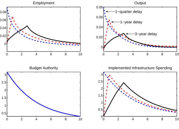
Leeper et al. (2010) estimate a dynamic model with government investment and contrast the impacts of higher infrastructure spending with different periods of implementation de-lays, the time between authorization and outlays. Figure 5 reports the estimated paths of employment and output following an injection of new infrastructure spending. The three lines in the figure are based on the same level of authorized spending, but represent differ-ent implemdiffer-entation delays: one-quarter delay (dashed lines), one-year delay (dotted-dashed lines), and three-year delay (solid lines). With a one-quarter delay, government investment today is transformed into public capital tomorrow, which raises employment and output immediately. With more plausible delays, such as a year, the boost to employment is also delayed and in the very short run, output may actually fall. As the implementation delay
0 2 4 6 8 10 0 0.02 0.04 0.06 0.08 Employment 0 2 4 6 8 10 0 0.02 0.04 0.06 0.08 Output 0 2 4 6 8 10 0.5 1 1.5 2 2.5 3 Budget Authority 0 2 4 6 8 10 0 0.5 1 1.5 2 2.5 3
Implemented Infrastructure Spending 1−quarter delay
1−year delay
3−year delay
Figure 5: Impacts of higher government investment under various lengths of implementation delays in a neo-classical growth model using post-war U.S. data. Dashed lines: one-quarter delay; dotted-dashed lines: one-year delay; solid lines: three-year delay. All variables are in percentage deviations from steady state. X-axis is in years. Source: Leeper et al. (2010).
grows, the short-run stimulus to employment and output becomes more muted. Delayed stimulus arises because private decisions depend on the timing with which infrastructure spending is expected to affect productivity.
Up to now, the discussion of multipliers has made no mention of monetary policy. In principle, though, the monetary policy stance can have major implications for fiscal impacts. Higher current and expected government spending, for example, will tend to raise current and expected inflation. If monetary policy is active and raises the nominal rate more than one-for-one with inflation, then real interest rates rise, inducing individuals to postpone consumption, offsetting some of the increase in demand for goods. On the other hand, passive monetary policy, which raises nominal rates only weakly with inflation, will tend to reduce real interest rates—government spending raises expected inflation, but the nominal rate now rises by less—and encourage higher current consumption. Recent research bears out this reasoning [Christiano et al. (2009), Erceg and Lind´e (2009), Eggertsson (2009), Davig and Leeper (2010b)].
similar to those in use at central banks, but in an environment in which monetary and fiscal policies are regularly switching between active and passive stances, as in Regimes M and F above. Davig and Leeper (2010b) use U.S. time series to estimate more general versions of the policy rules in section III, where the coefficients on the rules can be different in different policy regimes. Those rules are then embedded in a dynamic optimizing model and the model agents form expectations over future policies using the probability distributions estimated for the policy rules. Because regimes recur, even if policies today are in Regime M, agents know that there is some probability policies will switch to Regime F in the future.
P V(ΔY) P V(ΔG) after
Regime 5 quarters 10 quarters 25 quarters ∞
M: AM/PF .79 .80 .84 .86
F: PM/AF 1.72 1.58 1.40 1.36
Table 2: Output multipliers for government spending from new Keynesian model with fluc-tuating monetary and fiscal policy rules. AM: active monetary policy; PM: passive monetary policy; PF: passive tax policy; AF: active tax policy. Source: Davig and Leeper (2010b).
Conditional on being in Regime M, the government spending multipliers are modest—less than unity—at all horizons [table 2, row labeled M: AM/PF]. These estimates are close to the ones that emerge from neo-classical growth models without monetary policy. But when monetary policy is passive, the same spending impulse is substantially more stimulative, with output multipliers nearly twice as large [row labeled F: PM/AF]. Accounting for monetary policy behavior, and modeling that behavior explicitly, is essential to determine the potency of fiscal policy.18
Multipliers in themselves are not directly interesting to policymakers. But multipliers are a critical input to predict a particular legislation’s consequences, about which policymakers
18“Modeling that behavior explicitly” means that the details of how monetary policy accommodation is
handled matter. In table 2, it is the policyrule that changes and, because agents know rules can change, possible fluctuations in rules are embedded in their expectations. An alternative modeling strategy would be to posit an active monetary policy rule, such asRt=R∗+α(πt−π∗) +εtwithα >1 andεtan exogenous stochastic process. In the face of a fiscal expansion, the modeler could suspend this rule temporarily by feeding in a sequence of εt’s that allow Rt to track any desired interest rate path. This is a completely different exercise than regime change because agents in the model base their expectations on the active monetary policy rule and the realized path of the nominal interest rate comes as a surprise to the agents. Substantive issues rest on the details of the thought experiment. Researchers are not always clear about how their experiments are conducted.