San Jose State University
SJSU ScholarWorks
Master's Projects Master's Theses and Graduate Research
Spring 5-22-2019
Graph Classification using Machine Learning
Algorithms
Monica Golahalli Seenappa
San Jose State University
Follow this and additional works at:https://scholarworks.sjsu.edu/etd_projects Part of theArtificial Intelligence and Robotics Commons
This Master's Project is brought to you for free and open access by the Master's Theses and Graduate Research at SJSU ScholarWorks. It has been accepted for inclusion in Master's Projects by an authorized administrator of SJSU ScholarWorks. For more information, please contact [email protected].
Recommended Citation
Seenappa, Monica Golahalli, "Graph Classification using Machine Learning Algorithms" (2019).Master's Projects. 725. DOI: https://doi.org/10.31979/etd.b9pm-wpng
Graph Classification using Machine Learning Algorithms
A Project Presented to
The Faculty of the Department of Computer Science San Jose State University
In Partial Fulfillment of the Requirements for
CS298
by
Monica Golahalli Seenappa Spring 2019
c ○2019
Monica Golahalli Seenappa ALL RIGHTS RESERVED
The Designated Project Committee Approves the Project Titled
Graph Classification using Machine Learning Algorithms
by
Monica Golahalli Seenappa
APPROVED FOR THE DEPARTMENTS OF COMPUTER SCIENCE
SAN JOSE STATE UNIVERSITY
Spring 2019
Dr.Katerina Potika Department of Computer Science
Dr.Sami Khuri Department of Computer Science
ABSTRACT
Graph Classification using Machine Learning Algorithms by Monica Golahalli Seenappa
In the Graph classification problem, given is a family of graphs and a group of different categories, and we aim to classify all the graphs (of the family) into the given categories. Earlier approaches, such as graph kernels and graph embedding techniques have focused on extracting certain features by processing the entire graph. However, real world graphs are complex and noisy and these traditional approaches are computationally intensive. With the introduction of the deep learning framework, there have been numerous attempts to create more efficient classification approaches.
For this project, we will be focusing on modifying an existing kernel graph convo-lutional neural network approach. Moreover, subgraphs (patches) are extracted from the graph using a community detection algorithm. These patches are provided as input to a graph kernel and max pooling is applied. We will be experimenting with different commu-nity detection algorithms and graph kernels and compare their efficiency and performance. For the experiments, we use eight publicly available real world datasets, ranging from bi-ological to social networks. Additionally, for these datasets we provide results using a baseline algorithm and a spectral decomposition of Laplacian graph for comparison pur-poses.
Keywords - Graph Kernels, Convolutional Neural Network, Community detec-tion, Spectral decomposition
ACKNOWLEDGMENTS
I am obliged to have worked under Dr.Katerina Potika as my advisor. Having taken "Design and Analysis of Algorithms" and "Social Network Analysis" under Dr. Potika, I was very much interested in working under her for my writing project. Her constant guidance and support helped me a lot.
I would also like to thank Dr.Sami Khuri and Dr.Robert Chun for providing valuable feedback.
TABLE OF CONTENTS
CHAPTER
1 Introduction . . . 1
1.1 Problem Statement . . . 2
1.2 Applications of the Graph Classification problem . . . 4
2 Related Work. . . 5
2.1 Graph Kernel methods . . . 6
2.2 Deep learning approaches . . . 7
3 Methodology . . . 9
3.1 Weisfeiler-Lehman Subtree Kernel . . . 9
3.1.1 Model . . . 10
3.2 Graph Embedding using Laplacian Decomposition . . . 13
3.2.1 Model . . . 13
3.3 Kernel Graph Convolutional Neural Network (CNN) Approach . . . 15
3.3.1 Model . . . 16
4 Experimental Evaluation . . . 20
4.1 Datasets . . . 20
4.2 Weisfeiler-Lehman Subtree Graph Kernel . . . 21
4.3 Graph Embedding using Laplacian Decomposition . . . 23
4.4 Kernel Graph Convolutional Neural Network (KG-CNN) . . . 29
LIST OF TABLES
1 Dataset statistics and properties. . . 22
2 Experimental accuracy with Weisfeiler-Lehman subtree Kernel. . . 22
3 Experimental accuracy of different models. . . 25
4 Accuracy with varying number of estimators in Random Forest model . 26 5 Accuracy with varying number of leaf samples in Random Forest model 27 6 Accuracy with varying maximum depth in Random Forest model . . . 28
7 Accuracy with bootstrap parameter in Random Forest model . . . 29
8 Experimental accuracy with shortest path kernel on KG-CNN. . . 33
9 Experimental accuracy with shortest path kernel on KG-CNN. . . 33
10 Experimental accuracy with WL subtree kernel on KG-CNN. . . 34
11 Experimental accuracy with WL subtree kernel on KG-CNN. . . 34
12 Experimental accuracy with combination of shortest path and WL sub-tree kernel on KG-CNN. . . 35
13 Experimental accuracy with combination of shortest path and WL sub-tree kernel on KG-CNN. . . 35
14 Comparison of accuracies with shortest path kernel, WL subtree kernel and their combination. . . 35
15 Comparison of accuracies from all three methods: WL subtree kernel, Graph embedding using spectral decomposition, Kernel graph convo-lutional neural network . . . 36
LIST OF FIGURES
1 Known examples of toxic and non-toxic compounds [1] . . . 2
2 Unknown samples yet to be classified as toxic or non-toxic compounds [1] . . . 3 3 Weisfeiler-Lehman Subtree kernel forℎ=1. Step 1 and Step 2 of
Algo-rithm 2. . . 11 4 Weisfeiler-Lehman Subtree kernel forℎ=1. Step 3 and Step 4 of
Algo-rithm 2. . . 12 5 Weisfeiler-Lehman Subtree kernel forℎ=1. After the completion of all
steps. . . 12 6 Schematic view of the model . . . 15
7 Overview of the Kernel graph CNN approach . . . 17
8 Interquartile range for different estimators in Random Forest model . . 26 9 Interquartile range for different leaf samples in Random Forest model . 27 10 Interquartile range for varying depth in Random Forest model . . . 28 11 Interquartile range for bootstrapping in Random Forest model . . . 29
CHAPTER 1 Introduction
Graphs can be used to represent most real-world data. Objects can be denoted as nodes of the graph and edges can be used to represent relationship between them. Graphs are used almost in every field. In social networks, graphs are used to provide online recom-mendations, implement newsfeed and calculate page rank [2]. In the field of neuroscience, neurons are denoted by nodes and connections between them as edges. These graphs are then used to analyse the functionality of brain networks [3]. In chemical engineering, co-valent structures are represented as graphs [4]. Hydrocarbon structure, protein structure are represented in the form of graphs in bioinformatics field [5]. There are many more applications in other fields. These prove the importance of working with graphs.
Graph mining involves various tasks such as node classification, graph classification, link prediction, graph embedding, community detection. Since the introduction of machine learning approaches, there have been many attempts to discover useful information present within a graph. For applying such algorithms to graph domain, there should exist mean-ingful ways to compute similarity measures between graphs. Graph problems are not easy to solve. For example, the problem of finding maximum number of common subgraphs is computationally intractable. But graph similarity can be computed in various ways and the similarity measures need not be exact [6]. Approximate similarity measures are suffi-cient to work on graph related tasks. Even though there is significant progress in the field of graph mining, extracting graph features that truly represent the underlying graph struc-ture still remains a challenge. In this project, we are focusing on the problem of graph classification.
1.1 Problem Statement
Graph classification is the problem of determining the category or target label of the graph. If we have a dataset consisting of many input graphs, the problem is to classify each of the graphs to their correct category or target label. For example, in the case of chemical compounds, nodes represent the atoms and edges represent bonds between the atoms. The classification problem might be to determine if the chemical compound is toxic or non-toxic by looking at its structure. The model would be trained with known examples of toxic and non-toxic compounds as indicated by Figure 1. When the model encounters an unknown or new sample, it should predict whether it is toxic or non-toxic as indicated by Figure 2.
Figure 1: Known examples of toxic and non-toxic compounds [1]
Real world graphs are large and complex. They are known to contain lot of noise elements as well. These noise elements do not add any valuable information. It is crucial to eliminate them, else they might introduce wrong insights. The classifier model should be capable of handling large graphs as well has eliminate insights obtained from noise elements. The model should be robust, efficient to compute and not consume too much space.
Figure 2: Unknown samples yet to be classified as toxic or non-toxic compounds [1]
Given a dataset of input graphs 𝐺 = {𝐺1, 𝐺2, 𝐺3, ..., 𝐺𝑁},and their corresponding labels, the task is to build a model that learns from these graphs and predicts the label of new, unseen graphs. Graph features are computed and compared to make prediction for these new graphs. A popular approach is the usage of graph kernels, which focuses on calculating occurrences of different patterns in the input graphs. These include counting shortest-paths, performing random walks on the graphs, etc. Graphs which share lot of features are considered as similar and are placed in the same category [7].
Following are few of the challenges encountered during dataset processing:
∙ If the dataset is partially labeled, learning from the input graphs might lead to inac-curate information.
∙ If dataset is collected from multiple sources, then aggregation can cause information inconsistency.
∙ If the dataset is collected using some hardware instruments, care must be taken to ensure these instruments are not faulty [8].
∙ Dataset collected might be huge. Processing it efficiently by eliminating noisy fea-tures might be difficult.
1.2 Applications of the Graph Classification problem
There is lot of ongoing research in the field of graph theory. There has been continuous efforts to develop new methods to improve performance. Since graphs can be used to model complex structures, we look at few of their applications.
1. Bioinformatics and Chemoinformatics: Some applications include predicting the function of a protein structure, predicting if the cells are cancerous or not, predicting if a protein is enzyme or not, checking the toxicity of a chemical compound.
2. Neuroscience: Graphs are used to analyse brain networks. Neurons are represented using nodes and the connection between neurons are represented by edges [3]. 3. Natural Language Processing: It is used to categorize different documents based on
the structure of the texts [9].
4. Social Network analysis: Users on social networking sites such as Facebook or LinkedIn are represented as nodes and the interaction between them is captured using edges. Such networks help in providing recommendations for a page or user account to follow [2].
In this project, we have performed experiments focusing on improving the graph spec-trum algorithm as well as kernel graph convolutional neural networks. We compare our results with a baseline algorithm using Weisfeiler-Lehman kernel.
CHAPTER 2 Related Work
Graphs have been of great interest for a long time. Most earlier approaches dealt with identifying if two graphs are identical or not. This problem is hard to solve and until recently it was not known to be either tractable or intractable. In 2016, the author of [10], showed that graph isomorphism can be solved in (𝑒𝑥𝑝((𝑙𝑜𝑔𝑛)𝑂(1)))time. That is, we can
compute if graphs are identical or not in quasipolynomial time. In our problem, we are not interested in knowing if two graphs have same structure or not. We want to explore if two graphs are similar. This paves path for finding a more faster, efficient approach for our classification.
There are many approaches proposed for the task. Initial approaches would make lot of assumptions about the dataset. Most of them lacked a proper embedding technique. They processed only few nodes which they assumed to be important and also had certain assumptions about the graph data like its labeled or unlabeled, weighted or unweighted. Embedding techniques should be good enough to capture the relationship between nodes and retain the structure of the graph [8].
Initial techniques focused on developing a greedy algorithm for comparison between the two graphs. To compare two graphs G and G’, all we had to do is search each subgraph from G in G’. If all the subgraphs are present, we would declare they are similar else they are not similar. With the advancements in machine learning, many attempts were made to incorporate them to the field of graphs. The most famous among these approaches is the use of graph kernel [9]. The kernel approach computes a similarity matrix internally and passes this to a classification algorithm. There are several kernels proposed over the past
few years. We have wide range of kernels ranging from Random walks, Shortest-path to Weisfeiler-Lehman kernels [11].
2.1 Graph Kernel methods
Until recently, graph kernels dominated the graph classification. All graph kernels are developed with the same generic idea. They are represented in the form of a matrix which can then be passed onto a kernel-based classifier. The challenge is to develop a kernel function which can be computed relatively faster. The similarity function need to be symmetric and positive semidefinite.
Random walks kernels are one of the oldest graph kernels proposed. The basic idea is to count the common walks in the graphs and compare them [12]. Product is computed between the two graphs called as direct product graph. But this method is too slow and its complexity amounts to 𝑂(𝑛6). The walks may iterate over the same nodes again and leads to tottering effect. Many approaches were later proposed to improve the random-walk kernel. Notable among them is the cyclic-pattern kernel [13]. In this method, a graph is decomposed into many cyclic patterns. We compare the two graphs by comparing the number of cyclic patterns which appear in both the graphs. Computation power involved is low, but it does not work well for all the graphs. It works good only in the presence of simple cycles.
Instead of focusing on walks, focus shifted to paths [14]. Label enrichment techniques were developed to improve runtime for especially graphs will simple labels [15]. Also, op-timizations were performed using Singluar Value Decomposition (SVD) to generate lower rank matrices. Linear-algebra concepts were applied along with Kronecker product to re-duce complexity to 𝑂(𝑛3). Another major graph kernel developed was the shortest-path
can be computed in𝑂(𝑛3).For a given graph, its all-pair shortest path matrix is computed.
Another improvement made was to compute only 𝑘-shortest paths instead. Though the runtime was improved, it was still not fast enough.
The Weisfeiler-Lehman kernel by [16], outperformed all the graph kernels developed till then on most standard datasets. Specifically, the subtree variant, compared each label of the graph by using a compressed form. Computation was low since the labels were compressed and hashing was done. Desiging the kernel function dictates how fast the method will perform. It’s crucial to develop a function which can computed easily. Many other kernels where developed later like the optimal assignment kernel and graphlet kernels.
2.2 Deep learning approaches
Though the runtime efficiency of graph kernels have been improved over time, it has not improved considerably for the past few years. With the rise of deep learning ap-proaches, many models are built with Convolutional Neural Networks (CNN) and Recur-rent Neural Networks (RNN) for graphs. These models are applied to the area of graphs.
In the case of graph kernels, deriving features at a lower runtimes is a challenge [17]. Real-world data contains noise and plenty of information which might not be useful for classification purposes. The model developed must be capable of extracting relevant features and filtering out the noise and redundant information. With the advancement in deep learning approaches, deep learning models have been applied to every field. There are various form of CNNs been developed for classification purposes. CNNs developed for graphs are addresses as Graph CNNs or GCNNs. In GCNNs, the graphs are transformed by applying a graph laplacian [18]. The idea is taken from signal processing domain [19]. For this purpose, the authors make use of fourier transformation and apply it to graphs.
The above model is extended by authors in [20]. The authors extract spectral features and apply CNNs. Also, in [21], the graph features are hashed and the node information is fed into a one-dimensional neural network. Molecular biology can also help to visualise the graph contents. For example, in [22], the graph represents the structre within a molecule. in [17], graphs are classified using histograms. The challenge with using a GCNN is defining the convolution operation. There might be loss of information. Since graphs are non-linear, care must be taken with convolving and pooling operations.
RNNs are useful when the network needs to remember a decision being made pre-viously. If the current decision take, affects the future decision, then the current decision must be fed into the network. Specifically, a variant of RNN called the Long-Short term memory (LSTM) can be used to retain information for a longer period of time [23]. At-tention models are good approaches to work with RNNs. They can be used to focus on a set of nodes and make a decision using only these important nodes. Attention-guided walk will help to choose these important nodes. Especially, when the graph is large and contains lot of noise, the walk can be trained to not traverse through these nodes. The explorer can be given a high probability transition to the important nodes in the graph.
CHAPTER 3 Methodology
Given a collection of graphs𝐺={𝐺1, 𝐺2, 𝐺3, ..., 𝐺𝑁}where each𝐺𝑖 = (𝑉𝑖, 𝐸𝑖)has
𝑉𝑖 vertices and𝐸𝑖 edges, and their target labels, the graph classification problem aims to classify unknown graphs into appropriate categories. We begin each of our approach by building a model trained on the input dataset. The model should capture the relationship between the structure of a graph and its target label. When the model is given an unlabeled graph as input, it should determine the correct category of the graph.
3.1 Weisfeiler-Lehman Subtree Kernel
Graph kernels are one of the most important approaches used for graph classification. There are several kernels available, but we will be using the WL Subtree kernel for our experiments. Graph kernels make use of the kernel trick to reduce dimensionality. In each step of the algorithm, labels of the node are renamed with a set of labels formed by combining the immediate neighbors. The labels are renamed to a compressed version. The steps are repeated until the two graph’s labels vary.
Graphs kernels are a supervised approach to perform classification. Typically, a kernel matrix is computed upon applying a graph kernel. This matrix is passed to a kernel-based machine algorithm like Support Vector Machines (SVM) to perform classification. The WL Subtree kernel is based on WL test for isomorphism between two graphs. The algorithm for WL isomorphism test is given in Algorithm 1.
The WL isomorphism test has a time complexity of𝑂(ℎ𝑚), whereℎis the number of iterations specified by the user.𝑂(𝑚)is the time required to determine the labels for
com-Algorithm 1One iteration of the 1-dimensional Weisfeiler-Lehman test of graph isomor-phism
1: Multiset-label determination
∙ Fori=0, set𝑀𝑖(𝑣) :=𝑙0(𝑣) = 𝑙(𝑣)2.
∙ Fori>0, assign a multiset-label𝑀𝑖(𝑣)to each node𝑣 in G and G’ which consists of the multiset{𝑙𝑖−1(𝑢)|𝑢∈𝑁(𝑣)}.
2: Sorting each multiset
∙ Sort elements in 𝑀𝑖(𝑣) in ascending order and concatenate them into a string
𝑠𝑖(𝑣).
∙ Add𝑙𝑖1(𝑣)as a prefix𝑠𝑖(𝑣)and call the resulting string𝑠𝑖(𝑣).
3: Label compression
∙ Sort all of the strings𝑠𝑖(𝑣)for allvfrom G and G’ in ascending order.
∙ Map each string𝑠𝑖(𝑣)to a new compressed label, using a function𝑓 : Σ* → Σ such that𝑓(𝑠𝑖(𝑣)) =𝑓(𝑠𝑖(𝑤))if and only if𝑠𝑖(𝑣) =𝑠𝑖(𝑤).
4: Relabeling
∙ Set𝑙𝑖(𝑣) :=𝑓(𝑠𝑖(𝑣))for all nodes in G and G’.
pressed sets. For sorting each of the label,𝑂(𝑚)operations are required. To compress the lables, further𝑂(𝑚)operations are required. Therefore, a total of𝑂(ℎ𝑚)operations are re-quired. From Algorithm 1, we see that there are four crucial steps involved in isomorphism test. Based on these steps, a WL Subtree kernel is formulated.
3.1.1 Model
WL Subtree kernel is an extension of the idea in Algorithm 1. We start with all the input graphs in the dataset. Algorithm 2 is used to compute the kernel.
In this case, the algorithm runs in 𝑂(ℎ𝑚) time. In the first step, we compute the multiset label 𝑙𝑖 for all the 𝑁 graphs within the dataset. All the graphs are processed simultaneously and operations are performed in parallel in all theℎiterations. We obtain the neighborhood set for a given node and concatenate all their names into a single string in
Algorithm 2 One iteration of the Weisfeiler-Lehman subtree kernel computation on 𝑁
graphs
1: Multiset-label determination
∙ Assign a multiset-label𝑀𝑖(𝑣)to each node𝑣 in G which consists of the multiset {𝑙𝑖−1(𝑢)|𝑢∈𝑁(𝑣)}.
2: Sorting each multiset
∙ Sort elements in 𝑀𝑖(𝑣) in ascending order and concatenate them into a string
𝑠𝑖(𝑣).
∙ Add𝑙𝑖−1(𝑣)as a prefix to𝑠𝑖(𝑣).
3: Label compression
∙ Map each string𝑠𝑖(𝑣)to a compressed label, using a hash function𝑓 : Σ* → Σ such that𝑓(𝑠𝑖(𝑣)) =𝑓(𝑠𝑖(𝑤))if and only if𝑠𝑖(𝑣) =𝑠𝑖(𝑤).
4: Relabeling
∙ Set𝑙𝑖(𝑣) :=𝑓(𝑠𝑖(𝑣))for all nodes in G.
the second step. The neighbors of a node are sorted before adding to the multiset using radix sort. 𝑓 is the function that represents the mapping of neighborhood strings to a compressed label. 𝑓can also be implemented using a perfect hash function. The time complexity would be linear and is equal to𝑂(𝑁 𝑛+𝑁 𝑚) = 𝑂(𝑁 𝑚).This denotes the sum of the length of the string an the current alphabet. In the third and fourth step, we are compressing the label and renaming it.
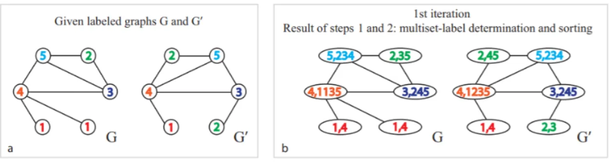
Figure 3: Weisfeiler-Lehman Subtree kernel forℎ=1. Step 1 and Step 2 of Algorithm 2.
both the graphs will have their own labels. We get a sorted list of neighbor for each node
𝑣𝑖 in the graph and replace the node’s label with this. This can be visualized in step 2. At the end of this iteration, both the graphs will have new long labels for each of their nodes.
Figure 4: Weisfeiler-Lehman Subtree kernel forℎ=1. Step 3 and Step 4 of Algorithm 2.
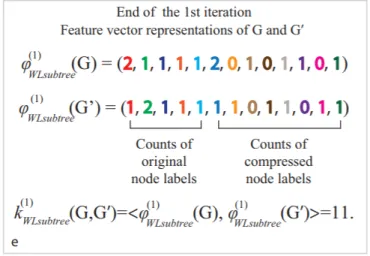
Since each node can have multiple neighbors, the string with which it is relabeled can be quite long. Therefore, in step 3, we focus on label compression. For each label in the graph, we replace it with a shorter label. This can be visualized in Figure 4.
Figure 5: Weisfeiler-Lehman Subtree kernel forℎ=1. After the completion of all steps.
With this, we complete the first iteration in our ℎ iterations. So at the end of each iteration, we would be computing a new feature vector for both the graphs. We compare the original graph with the new graph. We count the labels newly formed. We initially set a
threshold for the labels. If the labels vary more than the given threshold, then the algorithm terminates and we say that the graphs are not identical. If not, we continue our iterations till we reachℎiterations.
3.2 Graph Embedding using Laplacian Decomposition
Since graph is non-linear, we need to extract features from the graph that captures information within it. There are several graph embedding techniques for the same purpose. Using these embeddings, the graphs are represented in the form of a vector or group of vectors. Working on vectors are convenient and easier than processing the entire graph. Also, most programming languages support several packages to transform vectors. There are several approches like DeepWalk and Node2Vec [24] that perform random walks on the graph to capture information about their neighborhood. The embeddings should capture meaningful information from the graphs such as the interaction between subgraphs and neighborhood information for a node.
There are mainly two kind of graph embeddings. One focuses on embedding the entire graph and the other embeds nodes. We will be working with the entire graph embedding to perform classifications. We perform experiments using the spectral features of a graph as descibed in [25]. We derive features from the graph spectrum and pass it as input to a classifier. We have experimented with various classifiers ranging from Support Vector Machines to Multi-layer Perceptrons.
3.2.1 Model
Assume we have a set of undirected and unlabeled collection of graphs 𝐺 = (𝑉, 𝐸). Compute a boolean adjacency matrix𝐴 ∈ {0,1}which indicates 1 if there exists an edge between two nodes or 0 otherwise. Similarly a degree matrix 𝐷 is constructed which
contains degrees for each node. We assume the graph is connected. If it is not, then we extract the largest connected component from the graph.
In [25], the authors define the normalized laplacian of a graph by
𝐿=𝐼 −𝐷−1/2𝐴𝐷−1/2,
where𝐴is the adjacency matrix and𝐷is the degree matrix. The pseudocode for the model is given in Algorithm 3. There are three steps involved to obtain the spectral features. Algorithm 3Spectral decomposition of graph Laplacian
1: For graph𝐺= (𝑉, 𝐸)with𝑉 vertices and𝐸 edges, derive the following: ∙ A boolean adjacency matrix𝐴∈ {0,1}|𝑉|×|𝑉|.
∙ A degree matrix𝐷=𝑑𝑖𝑎𝑔(𝐴1)of node degrees.
2: Derive normalized laplacian for the graph
∙ If𝐺is not connected, then extract the largest connected component. ∙ Compute laplacian of𝐺as: 𝐿=𝐼 −𝐷−1/2𝐴𝐷−1/2
3: Derive spectral features of the graph
∙ Perform eigenvector decomposition on the graph and obtain𝑘 smallest positive eigenvalues of𝐿.
∙ If graph has less than𝑘nodes, pad zeroes to the right end of the vector.
4: Provide the spectral features as input to the classifier.
The Laplacian matrix computed might be huge for large graphs. Instead of considering the entire L matrix, we can focus only on the relevant elements which give us information about the graph. For this, we perform eigen decomposition of the matrix. The L matrix is now split into eigenvectors and eigenvalues. We chose the eigenvector which is the largest and its corresponding eigenvalue. The spectral features are defined by the eigenvlaues. These form the basis for comparison between two graphs. If the graphs are similar, then their corresponding eigenvectors are similar. They might just be a permutation of one another.
The spectral features are crucial for detecting similarity between graphs. From the eigenvalue decomposition performed earlier, we will choose only the𝑘 smallest eigenval-ues. These eigenvalues need to be positive as well. If there are less than𝑘eigenvalues, we append required number of zeroes to the vector. Finally, we sort the values. This vector represents the information in the graph. This is provided as input to a chosen classifier.
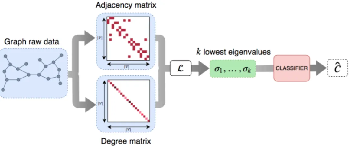
Figure 6: Schematic view of the model
Figure 6 demonstrates the above mentioned process. The method is fast and compara-ble with benchmark algorithms. Since the eigenvalues of the laplacian matrix lies between 0 and 2, preprocessing of the graph wouldn’t take much time and therefore the model is fast.
3.3 Kernel Graph Convolutional Neural Network (CNN) Approach
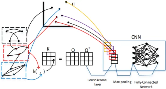
Deep learning has rose to prominence in the recent years. CNNs have been very successful for working with images and grid-like structures. For using CNNs, graphs need to be represented in the form of a vector or group of vectors. The KG-CNN approach works on the idea similar to CNNs.
we make use of a community detection algorithm. In the second stage, we have to normal-ize the communities. We make use of graph kernels here. After performing normalization, in the third stage, we pass the obtained vector through a CNN to predict label of the graph.
3.3.1 Model
Neural network models are efficient in extracting implicit features from data. But they accept inputs in the form of images or grids. They are mostly used in the areas of image recognition and image processing. If we have to use CNNs in our experiments, then we need to represent them in a form accepted by the CNNs. This embedding is done using graph kernels.
The approach used is described in Algorithm 4. Algorithm 4Kernel Graph CNN approach
1: Patch extraction on input Graph𝐺={𝐺1, 𝐺2, 𝐺3, ..., 𝐺𝑁} ∙ Applycommunity detectionalgorithm to extract patches. ∙ Subgraphs obtained form the set𝑆 ={𝑆1, 𝑆2, ..., 𝑆𝑁}.
2: Patch Normalization
∙ Apply the Nystrom method to obtain low-dimensional representations of the sub-graphs.
3: 1D Convolution
∙ Perform inner-product between the graph and the normalized patch. ∙ Convolving𝑤with all the normalized patches, feature map
𝑐= [𝑐1, 𝑐2, ....𝑐𝑃𝑚𝑎𝑥]
𝑇is produced.
4: Pooling
3.3.1.1 Patch Extraction
We refer to the subgraphs extracted from the graph as patches. We make use of several community detection algorithms to generate these subgraphs or patches. Before passing the graph to a CNN, we need to represent it in the form of a vector.
There are several ways to embed a graph. One could extract information from neigh-bors of a node and use it to form a vector. A random walk could be performed on the graph to extract relevant information. Care must be taken to make these approaches tractable. With random walk we need to be careful not to loop within the same set of nodes. In our approach, we make use of community detection algorithms to identify the subgraphs. Nodes which are densely connected to one another are considered to interact with each other a lot and produce good partitions within the graph. Based on the algorithm chosen, outliers maybe eliminated from the partition process.
3.3.1.2 Patch Normalization
We have a set of subgraphs𝑆 ={𝑆1, 𝑆2, ..., 𝑆𝑁}obtained from the previous stage. To pass these patches to a CNN, we need to normalize them. For this purpose, we make use of the well-known graph kernels.
Suppose, if
𝐺=𝐺1, 𝐺2, 𝐺3, ..., 𝐺𝑁 are the input graphs within a dataset, and
𝑆 =𝑆1, 𝑆2, 𝑆3, ..., 𝑆𝑀
are the communities derived from the input graph G. Based on the community detection algorithm used, the number of subgraphs obtained will vary.
Let 𝑆𝑖𝑗 be the 𝑗𝑡ℎ subgraph extracted from 𝐺
𝑖. Let the total number of subgraphs extracted from𝐺𝑖 be𝑃𝑖. Let P be the cardinality and𝐾 ∈𝑅𝑃*𝑃 be the symmetric positive semidefinite kernel matrix constructed from S using a graph kernel𝑘.
The kernel matrix to be populated can be very huge. In order to obtain low-dimensional representations, the Nystrom method is used. We work with a small subset of the graph at a time, rather than using the entire input collection of graphs.
3.3.1.3 Graph processing
After the patches are normalized, the vectors can now be processed by a 1D CNN. There are mainly two steps involved when we use a CNN:
∙ Convolution: It is mainly used to extract features from the input. In traditional image processing scenario, an image pixel with multiplied with a filter, to obtain a single feature. Convolution is basically convolving two data, that is trying to merge two sets
of information in a way as to obtain meaningful information. In our experiments, we perform convolution between the extracted patches and the input graph dataset. This product is computed by the use of a graph kernel. By performing this convolution, we obtain a feature map. This feature map represents information of the patches in the graph.
∙ Pooling: To reduce the computation, we define a pooling layer. This layer performs computation on each feature vector. We apply specifically a max-pooling function over the obtained feature map. The function retains only the maximum value. This reduces computation and additional storage, since we are only interested in the max-imum value.
CHAPTER 4 Experimental Evaluation 4.1 Datasets
We will be working with eight publicly available real-world datasets. The description of these datasets are as follows:
∙ NCI-1: Lung Cancer data with 1793 positives, 37349 total graphs for non-small cell lung. Data made publicly available by NCI [26].
∙ MUTAG: 188 mutagenic aromatic and heteroaromatic nitro compounds with 7 dis-crete labels.
∙ PTC: (Predictive toxicology Challenge) 344 chemical compounds that reports the carcinogenicity for male and female rats and has 19 discrete labels.
∙ ENZYMES: Balanced dataset of 600 proteins tertiary structures and has three dis-crete lables (helix, sheet or turn).
∙ PROTEINS: Classifiable as enzymes or non-enzymes. Proteins are represented as graphs with nodes as secondary structure elements (SSEs), which are connected whenever they have neighbors either in the amino acid sequence or in 3D space. ∙ IMDB-BINARY: 1000 graphs of movie collaboration ego-networks. The task is to
classify an actor to his genre. The genres are comedy and action. The ego-network is built by placing each actor as node. Edges exist if two actors have worked in the same movie. If a movie can be classified into more than one genre, then we give priority to action.
∙ IMDB-MULTI: This dataset is generated in the same way as IMDB-BINARY. The only difference is it has multiple labels. The genre includes sci-fi along with comedy and romance. The dataset contains 1500 graphs [11].
∙ DD: Contains two types of graphs. One represents enzyme structure and the other represents non-enzyme structure. It contains close to 1200 graphs and each graph is very large containing close to 241 nodes per graph.
The above benchmark datasets for graph kernels are collected from [27]. If 𝑛 is the number of nodes,𝑚is the number of edges, and𝑁is the number of graphs, then the dataset contains files with the following format:
∙ DS_A.txt: Contains 𝑚 lines corresponding to entries of edge. Since the graph is undirected, it contains two entries for each edge.
∙ DS_graph_indicator.txt: 𝑛 lines where the value in 𝑖-th line is the graph_id of the node with node_idi.
∙ DS_graph_labels.txt: 𝑁 lines where the 𝑖-th line is the class label of the graph with graph_id𝑖.
∙ DS_node_labels.txt:𝑛lines where the value in𝑖-th line corresponds to the node with node_id𝑖.
4.2 Weisfeiler-Lehman Subtree Graph Kernel
The graph kernel approach is used as a baseline for our experiments. There are many graph kernels available: Random Walk, Shortest-Path, Weisfeiler-Lehman, Optimal As-signment, Weighted Decomposition and many more. Among these kernels, Weisfeiler-Lehman subtree kernel provides competitive results. It’s accuracy levels are comparable to
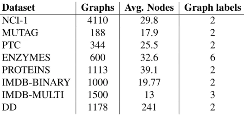
Table 1: Dataset statistics and properties.
Dataset Graphs Avg. Nodes Graph labels
NCI-1 4110 29.8 2 MUTAG 188 17.9 2 PTC 344 25.5 2 ENZYMES 600 32.6 6 PROTEINS 1113 39.1 2 IMDB-BINARY 1000 19.77 2 IMDB-MULTI 1500 13 3 DD 1178 241 2
benchmark models and its runtime is faster for smaller datasets. For the above reasons, we have used Weisfeiler-Lehman (WL) subtree kernel as our baseline algorithm.
For implementing this kernel, I have made use of the popular Python package "graphk-ernels". The package contains an interface to a C++ code that provides an implementation of the WL-subtree kernel. All we need to do was set the maximum number of iterationsℎ, and specify the dataset. Internally, the package constructs a kernel matrix for the collection of input graphs. The kernel matrix is constructed using the WL subtree kernel and later passed as input to SVM classifier to train the model.
Table 2: Experimental accuracy with Weisfeiler-Lehman subtree Kernel.
Dataset Accuracy NCI-1 80.13 MUTAG 82.05 PTC 56.97 ENZYMES 52.22 PROTEINS 72.92 IMDB-BINARY 68.6 IMDB-MULTI 48.13 DD 71.3
Table 2 provides a summary of accuracies achieved with the WL subtree kernel. These results will be used as a baseline for our graph embedding and kernel graph convolutional
neural network method.
4.3 Graph Embedding using Laplacian Decomposition
We have used the eight datasets described previously for our experiments. For building the classifiers, we make use of the machine learning library scikit-learn in Python. The classifiers used for obtaining the results are as follows:
1. AdaBoost (AB) Classifier - A boosting algorithm attempts to improve performance of several weak classifiers by combining them. It tries to create a strong classifier. AdaBoost is one the most successful boosting algorithm. Usually, decision tree with one level is used with AdaBoost to enhance the model performance.
2. Multilayer Perceptron (MLP) Classifier - MLP is a feedforward deep artificial neural network model. It consists of an input layer to receive the inputs, output layer which predicts the result and an arbitrary number of hidden layers that maps inputs to out-puts. In our experiments, we have used limited-memory BFGS (Broyden-Fletcher-Goldfarb-Shanno) algorithm for parameter estimation since it is an optimization al-gorithm and consumes less memory.
3. 𝑘-Nearest Neighbors (𝑘-NN) Classifier - An entity is classified by the number of votes received from its neighbors. Based on the category of majority of its neighbors, the entity or object is classified. Here,𝑘denotes the number of neighbors to take into account.
4. Gaussian Naive Bayes (GNB) Classifier - This classifier assumes that all features are independent of each other and is based on the popular "Bayes theorem". The Gaussian form is used when features follow normal distribution and have continuous values.
5. Decision Tree (DT) Classifier - It constructs a model by learning certain "decision rules". It is constructed using a tree representation where the internal nodes indicate features and the leaves indicate a class label. At the root of the model, the best attribute of the dataset is placed.
6. Random Forest (RF) classifier - It is an ensemble algorithm that combines many de-cision trees. It is trained using the bagging method, where a combination of dede-cision trees is used to increase the accuracy. Each decision tree votes and the final class of the graph is determined using the majority vote.
7. Support Vector Machine (SVM) Classifier - SVM tries to find a hyperplane which separates input graphs belonging to separate classes. It is a non probabilistic linear classifier which employs kernel trick to map input features into high dimensional spaces.
8. Logistic Regression (LR) - It is most widely used for binary classification problems. Logistic function is the core of this method. Logistic regression transforms its output using the logistic sigmoid function to return a probability value which can then be mapped to two or more discrete classes [28].
Hyperparameters were tuned to obtain better results with each classifier. The embedding dimension is set to the average number of nodes for each dataset. To compute accuracy of the model, 𝑘-fold cross validation is used. We have set𝑘=10 for our experi-ments. This means the dataset is divided into ten folds. Nine of the folds act as training set, while the remining one is the test set. This is repeated for all the 10 folds and the accuracy of the model is the average value across all the folds. The results for each of the classifier is tabulated in Table 3.
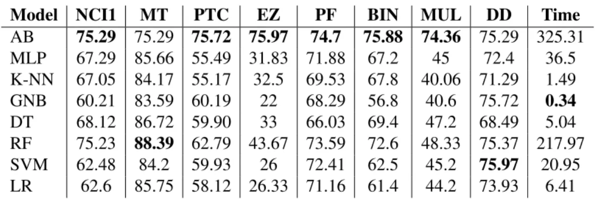
Table 3: Experimental accuracy of different models.
Model NCI1 MT PTC EZ PF BIN MUL DD Time
AB 75.29 75.29 75.72 75.97 74.7 75.88 74.36 75.29 325.31 MLP 67.29 85.66 55.49 31.83 71.88 67.2 45 72.4 36.5 K-NN 67.05 84.17 55.17 32.5 69.53 67.8 40.06 71.29 1.49 GNB 60.21 83.59 60.19 22 68.29 56.8 40.6 75.72 0.34 DT 68.12 86.72 59.90 33 66.03 69.4 47.2 68.49 5.04 RF 75.23 88.39 62.79 43.67 73.59 72.6 48.33 75.37 217.97 SVM 62.48 84.2 59.93 26 72.41 62.5 45.2 75.97 20.95 LR 62.6 85.75 58.12 26.33 71.16 61.4 44.2 73.93 6.41
We can notice that Random Forest classifier gives very good results. AdaBoost classi-fier was first constructed with decision trees. But upon replacing it with Random Forest as weak learner, we get better results. For getting the right parameters, we focus on Random Forest classifier and vary the depth, number of observations and estimators. We can choose the exact value of each hyperparameter and pass this to our AdaBoost classifier.
Random forest is an ensemble method that makes use of lot of decision trees to make classification. We start with increasing the number of trees in our model. With increase in number of trees, we can get better accuracy until a point, after which the model tends towards overfitting and the computation speed also declines. This is supported by our observations in Table 4. We have performed experiments using then_estimatorsparameter. Aftern_estimators = 500, we do not obtain increase in performance. Infact, the accuracy of the model begins to slide downward due to overfitting.
Also, we have varied the leaf size, that is the number of cases or observations in the leaf node. A fully-grown tree is a deep tree in a Random Forest that has only one data point in the leaf. Deep trees generally overfit the model since they have low bias and high
Table 4: Accuracy with varying number of estimators in Random Forest model
Estimators NCI1 MT PTC EZ PF BIN MUL DD
1 65.03 83.67 59.06 30 61.9 67.4 46.6 67.23 10 72.79 84.67 61.66 37.16 70.08 70.5 48.06 73.51 50 74.37 86.28 62.23 42.33 72.24 72.7 47.46 75.21 100 74.18 87.33 63.07 41.16 72.6 72.9 48 75.89 250 75.01 87.86 62.5 42.5 72.87 72.9 48.06 75.63 500 75.23 88.39 62.22 42.16 73.5 73.1 48.06 75.63 750 75.01 87.89 61.37 42.67 73.5 72.9 47.73 75.8 1000 74.98 87.36 61.07 42.16 73.41 72.8 47.73 75.8
Figure 8: Interquartile range for different estimators in Random Forest model
variance. But when we combine several deep trees, the variance is reduced [29]. From table 5, we can notice that when the leaf sample is 1, high accuracy is obtained for five out of seven datasets.
The depth of the tree is varied using themax_depthparameter and the corresponding accuracy’s are documented in Table 6 and interquartile ranges in Figure 10. When we increase the number of splits in a tree, it can capture the information well. We fit the trees with depth varying from 1 to 1000. The model attains it’s maximum accuracy at depth 50.
Table 5: Accuracy with varying number of leaf samples in Random Forest model
Leaf Samples NCI1 MT PTC EZ PF BIN MUL DD
1 75.23 88.39 62.22 42.16 73.5 73.1 48.06 75.8 2 74.67 87.89 60.52 41 73.77 73.3 47.66 75.8 3 74.57 88.39 60.8 39.33 74.13 72.8 47.86 75.97 4 74.47 87.89 61.37 38.5 74.22 72.5 48.26 75.46 5 73.6 87.33 61.66 37.83 73.95 72.7 49 75.89 6 73.55 85.16 61.97 36.5 73.95 72.7 48.4 75.29
Figure 9: Interquartile range for different leaf samples in Random Forest model
The results do not show improved accuracy even when we increase depth to 1000.
Next, we experiment with bootstrapping. Many classifier models are sensitive to the data they are trained on. Speficially, decision tree model generates different trees with different data. To avoid this high variance, we use a technique called bootstrapping. There is no need to generate additional training data. The dataset we have is randomly sampled. We chose different segments within the data and replace it for experiments. Each of the model generated with different segments of dataset are not correlated.
multi-Table 6: Accuracy with varying maximum depth in Random Forest model
Depth NCI1 MT PTC EZ PF BIN MUL DD
1 61.75 84.61 59.33 25.16 72.06 64 44.53 75.29 5 68.7 87.89 61.06 35.16 73.23 70.9 48.33 74.87 10 73.42 88.39 60.49 43 73.68 73.6 48.53 75.63 50 75.23 88.39 62.22 42.16 73.5 73.1 48.06 75.8 100 75.23 88.39 62.22 42.16 73.5 73.1 48.06 75.8 250 75.23 88.39 62.22 42.16 73.5 73.1 48.06 75.8 500 75.23 88.39 62.22 42.16 73.5 73.1 48.06 75.8 750 75.23 88.39 62.22 42.16 73.5 73.1 48.06 75.8 1000 75.23 88.39 62.22 42.16 73.5 73.1 48.06 75.8
Figure 10: Interquartile range for varying depth in Random Forest model
ple datasets. Therefore, we create an illusion that the model is trained on multiple datasets. Random forest is built so that each decision tree within the forest reduces the variance of the model and improves performance.
When we choose the data to run our model on, the remaining samples form the OOB (Out-of-Bag samples). Each model’s performance is evaluated on these OOBs. The overall performance is the average result obtained. Each of these performance measure is obtained
Figure 11: Interquartile range for bootstrapping in Random Forest model
using𝑘-fold cross validation. The accuracy of the model with and without bootstrapping is tabulated in Table 7.
Table 7: Accuracy with bootstrap parameter in Random Forest model
Bootstrap NCI1 MT PTC EZ PF BINARY MULTI
False 75.1 86.8 62.22 42.5 72.78 71.4 47.6
True 75.23 88.39 62.22 42.16 73.5 73.1 48.06
By performing the above experiments, we set the following hyperparamters for the Random forest classifier within AdaBoost: Number of estimators is 500, number of leaf samples is 1 and maximum depth is 50. In Table 3, we can notice that the AdaBoost classifier outperforms other classifiers on six datasets.
4.4 Kernel Graph Convolutional Neural Network (KG-CNN)
The first step in any machine learning algorithm is to extract features from the input dataset. In KG-CNN method, the feature extraction is done using community-detection
algorithms. We extract only the nodes which contain high information. These subgraphs or communities can be extracted using any community detection algorithm. In the paper [9], the authors have made use of the louvain clustering algorithm for experiments. We experi-ment with other well known community detection algorithms from the well-knownigraph package.
1. Louvain algorithm: It is a well-known bottom-up approach algorithm. It is based on greedy paradigm and works well for larger datasets. The algorithm proceeds by forming communities unless it can no longer increase the modularity of the net-work formed. It was developed by the University of Louvain. Nodes are assigned to different communities and the algorithm checks if it a right choice by computing modularity. If modularity has increased, the it continues otherwise it stops.
2. Spinglass algorithm: If the network contains overlapping communities, then it is quite difficult to separate them. Spinglass works well with networks that contain lot of noise. It can distinguish structures well even when there are overlapping com-munities. It is a semi-supervised model. The noise is filtered out during formation of communities. Guidance parameter is added to speedup the performance of the model.
3. Walktrap algorithm: This algorithm is based on random walks. We start from an intial node and perform random walks to its neighbors. These walks are helpful to capture the similarities between nodes, if it exists. Communities are formed between similar nodes. During the walk, a distance parameter is computed which helps in forming the clusters. It is an agglomerative approach which uses the distance parameter for building clusters. The distance is easy to compute, which makes the algorithm fast for usage.
4. Fast greedy algorithm: It works similarly to Louvain clustering algorithm. It tries to maximize the modularity score achieved. This algorithm basically works on the idea to eliminate outliers present with a cluster. It forms strongly connected components at the end of its iteration by achieving a maximum entropy. If the user mentions paramter𝑘, the number of outliers to eliminate from the network, then it elimiates𝑘
nodes from the communities formed.
5. Eigen vector algorithm: For the given input dataset, containing a collection of graphs, the algorithm begins by constructing a modularity matrix,𝑀 =𝐴−𝑃, where𝐴is the boolean adjacency matrix. 𝑃 denotes a probability matrix which indicates the probability with which each pair of edges are commected. For these matrices, eigen-vector is computed. The number of clusters is determined by this eigeneigen-vector. If the eigenvector contains all elements with same sign, then it indicates that communities cannot be formed. Each community is formed by distinguishing the different signs present between neighbors in the eigenvector.
6. Infomap algorithm: This algorithm tries to reduce runtime by making use of compression labels similar to Huffman code. The information is compressed before passing it to a random walk explorer. This explorer is responsible for forming the partitions in the graph. The information obtained by this explorer is also compressed. The movement of explorer to each node within the graph can be represented by a Markov transition matrix. At each step in the algorithm, the node labels are compressed. If there are spider-traps within a network, that is, if the random walk explorer cannot come out of a group of nodes, then we can substitute this group with a compressed label. At each step of the algorithm, we find this group of nodes and relabel them with a unique code.
7. Label propagation algorithm: It is a semi-supervised algorithm. The algorithm be-gins with a small set of nodes in the graph. It relabels all these nodes. The labels are then propagated along other nodes during different iterations in the algorithm. The algorithm runs pretty fast. The number of labels to provide initially can be deter-mined by the user. These labels indicate the number of communities to be formed at the end. Since in each iteration, we do not add additional labels, we only have the initial set of labels to consider for the entire graph.
8. Multilevel algorithm: This algorithm works in multiple stages. In each stage, the number of nodes in the graph to work with, is reduced. It continuously refines the nodes and edges and creates clusters, then maps them back to the original graph. There are various refinement approaches available. Based on the approach chosen, the results achieved could be quite high and also the algorithm works pretty fast. 9. Optimal modularity algorithm: This algorithm is very slow when compared to the
above mentioned algorithms. It again works on the principle of a modularity mea-sure. It tries to maximize this measure in the current iteration. The way this is handled is representing the problem as an integer programming problem.
After we form communities by using any of the above mentioned community detection al-gorithms, we have to normalize them. We denote the communities as patches or subgraphs. We use graph kernels for this purpose. As we discussed earlier, there are multiple graph kernels available. For our experiments, we have used two different types of kernels. First one is the shortest path kernel and the second is the WL subtree kernel discussed in Section 3.2.
The shortest path kernel begins by computing shortest path between two graphs. For this, we use the all-pair shortest path algorithm by Floyd-Warshall. The kernel is defined
on this shortest-path matrix.
Table 8: Experimental accuracy with shortest path kernel on KG-CNN.
Dataset Louvain Spinglass Walktrap Fastgreedy
NCI-1 74.52 N/A N/A 73.55
MUTAG 81.9 85.08 82.39 74.59 PTC 53.78 53.2 53.56 57.88 ENZYMES 38 N/A 46.35 39.83 PROTEINS 71.78 unconnected 72.85 73.05 IMDB-BINARY 70.7 69.2 70.3 70.6 IMDB-MULTI 46.2 46.53 47.93 47.8 DD 75.21 unconnected 75.63 75.63
Table 9: Experimental accuracy with shortest path kernel on KG-CNN.
Dataset Eigenvector Infomap Label Prop Multilevel
NCI-1 75.03 75.96 68.04 76.32 MUTAG 79.23 81.4 73.39 83.01 PTC Max. Iter 59.62 52.36 56.66 ENZYMES 37.16 39 31.83 36.66 PROTEINS 72.23 72.14 72.06 72.5 IMDB-BINARY N/A 70.1 69.2 66 IMDB-MULTI 42.93 39.73 33.8 40.66
DD Max. iterations No memory No memory 74.87
Table 8 and Table 9 indicate the accuracy of our method using only shortest path kernel for patch extraction.
Table 10 and Table 11 indicate the accuracies obtained with WL Subtree kernel. Com-paring them with the results obtained from the shortest-path kernel, we can see that there is not much difference between using shortest-path and WL kernel. So for the next phase of experiments, we have combined both the kernels to see if there is an improvement in the results.
From Table 12 and Table 13, we can notice that there is slight improvement in accura-cies when we combine the kernels as compared to using only either the shortest path kernel
Table 10: Experimental accuracy with WL subtree kernel on KG-CNN.
Dataset Louvain Spinglass Walktrap Fastgreedy
NCI-1 75.83 N/A N/A 74.11
MUTAG 81.46 84.59 79.85 75.61 PTC 57.57 56.12 57.54 56.74 ENZYMES 38 N/A 43.2 39.83 PROTEINS 71.78 unconnected 72.85 73.05 IMDB-BINARY 70.7 69.2 70.3 70.6 IMDB-MULTI 46.2 46.53 47.93 47.8 DD 76.82 unconnected 74.79 75.46
Table 11: Experimental accuracy with WL subtree kernel on KG-CNN.
Dataset Eigenvector Infomap Label Prop Multilevel
NCI-1 74.47 76.86 67.63 76.03 MUTAG 79.32 78.8 79.96 80.35 PTC Max. Iter 57.87 56.07 62.3 ENZYMES 37.16 39 31.83 36.66 PROTEINS 74.03 unconnected 73.48 73.49 IMDB-BINARY 69.6 67.89 72.3 71.3 IMDB-MULTI 47.26 47.53 46.89 27.88
DD Max. iterations No memory No memory 74.44
or WL kernel.
From Table 14, we can notice slight improvements in six out of eight datasets. This is because we have used a different community detection algorithm and combination of graph kernels. Multilevel algorithm performs better overall than the louvain clustering algorithm described in [9].
Table 12: Experimental accuracy with combination of shortest path and WL subtree kernel on KG-CNN.
Dataset Louvain Spinglass Walktrap Fastgreedy
NCI-1 74.52 N/A N/A 73.55
MUTAG 81.9 85.08 82.39 74.59 PTC 53.78 53.2 53.56 57.88 ENZYMES 38 N/A 48.12 39.83 PROTEINS 69.72 73.21 71.78 72.05 IMDB-BINARY N/A 70.5 70.7 72.6 IMDB-MULTI 46.39 45.13 48.99 47.13 DD 77.5 unconnected 75.13 76.56
Table 13: Experimental accuracy with combination of shortest path and WL subtree kernel on KG-CNN.
Dataset Eigenvector Infomap Label Prop Multilevel
NCI-1 75.03 75.96 68.04 76.86 MUTAG 79.23 81.4 73.39 83.01 PTC Max. Iter 59.62 52.36 62.2 ENZYMES 37.16 39 31.83 36.66 PROTEINS 72.23 72.14 72.06 72.5 IMDB-BINARY N/A 71 70.1 71.4 IMDB-MULTI 48 48.13 48 48.13
DD Max. iterations No memory No memory 78.83
Table 14: Comparison of accuracies with shortest path kernel, WL subtree kernel and their combination.
Dataset Shortest path WL kernel Shortest path + WL Results from related work [9]
NCI-1 76.32 76.86 76.86 77.21 MUTAG 85.08 84.59 85.08 N/A PTC 59.62 58.42 62.3 62.05 ENZYMES 46.35 43.2 48.12 48.12 PROTEINS 73.05 74.03 73.21 73.79 IMDB-BINARY 70.7 72.3 72.6 71.45 IMDB-MULTI 47.93 47.93 48.99 47.46 DD 75.63 76.82 78.83 78.83
CHAPTER 5
Conclusions and Future Work
We have performed extensive experiment’s on the graph decomposition using graph laplacian and kernel graph convolutional neural network (KG-CNN) methods. For the graph decomposition method, we have made use of several supervised learning algorithms available in thescikit-learnpackage. For the KG-CNN method, we performed experiments with different community-detection algorithms. Upon comparing all the three methods, we find that graph embedding using laplacian decomposition performs well onfiveout of eight datasets. We obtained this result when we used AdaBoost classfier.
Table 15: Comparison of accuracies from all three methods: WL subtree kernel, Graph embedding using spectral decomposition, Kernel graph convolutional neural network
Dataset WL subtree kernel Graph embedding KG-CNN
NCI-1 80.13 75.29 76.86 MUTAG 82.05 75.29 85.08 PTC 56.97 75.72 62.3 ENZYMES 52.22 75.97 48.12 PROTEINS 72.92 74.7 73.21 IMDB-BINARY 68.6 75.88 72.6 IMDB-MULTI 48.13 74.36 48.99 DD 71.3 75.29 78.83
For future work, we can try to reduce the execution time by introducing parallelism in the code. Also, we could perform patch normalization using different combination of graph kernels and try to increase performance of the model.
LIST OF REFERENCES
[1] N. Samatova. “Graph classification.” 2015. [Online].
Avail-able: https://www.csc2.ncsu.edu/faculty/nfsamato/practical-graph-mining-with-R/slides/pdf/Classification.pdf
[2] L. Tang and H. Liu, “Graph mining applications to social network analysis,” in Man-aging and Mining Graph Data, 2010, pp. 487–513.
[3] J. O. Garcia, A. Ashourvan, S. Muldoon, J. M. Vettel, and D. S. Bassett, “Applications of community detection techniques to brain graphs: Algorithmic considerations and implications for neural function,”Proceedings of the IEEE, vol. 106, no. 5, pp. 846– 867, 2018.
[4] S. J. Kulkarni, “Graph theory: Applications to chemical engineering and chemistry,” Galore International Journal of Applied Sciences and Humanities, vol. 1, no. 2, 2017. [5] G. A. Pavlopoulos, M. Secrier, C. N. Moschopoulos, T. G. Soldatos, S. Kossida, J. Aerts, R. Schneider, and P. G. Bagos, “Using graph theory to analyze biological networks,”BioData Mining, vol. 4, p. 10, 2011.
[6] N. M. Kriege and P. Mutzel, “Subgraph matching kernels for attributed graphs,” in Proceedings of the 29th International Conference on Machine Learning, ICML 2012, Edinburgh, Scotland, UK, June 26 - July 1, 2012.
[7] D. Rogers and M. Hahn, “Extended-connectivity fingerprints,” Journal of Chemical Information and Modeling, vol. 50, no. 5, pp. 742–754, 2010.
[8] M. Neumann, R. Garnett, C. Bauckhage, and K. Kersting, “Propagation kernels: effi-cient graph kernels from propagated information,”Machine Learning, vol. 102, no. 2, pp. 209–245, 2016.
[9] G. Nikolentzos, P. Meladianos, A. J. Tixier, K. Skianis, and M. Vazirgiannis, “Ker-nel graph convolutional neural networks,” inArtificial Neural Networks and Machine Learning - ICANN 2018 - 27th International Conference on Artificial Neural Net-works, Rhodes, Greece, October 4-7, 2018, Proceedings, Part I, 2018, pp. 22–32. [10] L. Babai, “Graph isomorphism in quasipolynomial time,” 2015.
[11] M. Zhang, Z. Cui, M. Neumann, and Y. Chen, “An end-to-end deep learning architec-ture for graph classification,” inProceedings of the Thirty-Second AAAI Conference on Artificial Intelligence, (AAAI-18), the 30th innovative Applications of Artificial
Intelligence (IAAI-18), and the 8th AAAI Symposium on Educational Advances in Ar-tificial Intelligence (EAAI-18), New Orleans, Louisiana, USA, February 2-7, 2018, pp. 4438–4445.
[12] H. Kashima, K. Tsuda, and A. Inokuchi, “Marginalized kernels between labeled graphs,” inProceedings of the International Conference on Machine Learning, 2003, pp. 321–328.
[13] T. Horvath, T. Gartner, and S. Wrobel, “Cyclic pattern kernels for predictive graph mining,” in Proceedings of the International Conference on Knowledge Discovery and Data Mining (KDD), 2004, pp. 158–167.
[14] S. Vishwanathan, N. Schraudolph, R. Kondor, and K. Borgwardt, “Graph kernels,” Journal of Machine Learning Research, vol. 11, no. 5, pp. 1201–1242, 2010.
[15] P. Mahe, N. Ueda, T. Akutsu, J. Perret, and J. Vert, “Extensions of marginalized graph kernels,” in Proceedings of the Twenty-First International Conference on Machine Learning, 2004, pp. 552–559.
[16] G. Nikolentzos, P. Meladianos, and M. Vazirgiannis, “Matching node embeddings for graph similarity,” pp. 2429–2435, 2017.
[17] A. Tixier, G. Nikolentzos, P. Meladianos, and M. Vazirgiannis, “Graph
classification with 2d convolutional neural network,” Jul. 2017. [Online]. Available: https://arxiv.org/abs/1708.02218
[18] J. Bruna, W. Zaremba, A. Szlam, and Y. LeCun, “Spectral networks and locally connected networks on graphs,” in 2nd International Conference on Learning Representations, ICLR 2014, Banff, AB, Canada, April 14-16, Conference Track Proceedings, 2014. [Online]. Available: http://arxiv.org/abs/1312.6203
[19] Shuman, I. David, S. Narang, K. Frossard, and V. Pierre, “The emerging field of signal processing on graphs: Extending highdimensional data analysis to networks and other irregular domains,” in. IEEE Signal Processing Magazine. IEEE, 2013, pp. 83–98. [20] M. Defferrard, X. Bresson, and P. Vandergheynst, “Convolutional neural networks on graphs with fast localized spectral filtering,” CoRR, vol. abs/1606.09375, 2016. [Online]. Available: http://arxiv.org/abs/1606.09375
[21] D. K. Duvenaud, D. Maclaurin, J. Aguilera-Iparraguirre, R. Gómez-Bombarelli, T. Hirzel, A. Aspuru-Guzik, and R. P. Adams, “Convolutional networks on graphs for learning molecular fingerprints,” pp. 2224–2232, 2015.
[22] A. Grover and J. Leskovec, “Scalable feature learning for networks,”KDD 2016 Pro-ceedings of the 22nd ACM SIGKDD, 2016.
[23] J. Lee, K. Rossi, S. Kim, and E. Koh, “Attention models in graphs: A survey.”
[24] A. Grover and J. Leskovec, “node2vec: Scalable feature learning for networks,” in Proceedings of the 22nd ACM SIGKDD International Conference on Knowledge Dis-covery and Data Mining, San Francisco, CA, USA, August 13-17, 2016, 2016, pp. 855–864.
[25] N. de Lara and E. Pineau, “A simple baseline algorithm for graph classification,” CoRR, vol. abs/1810.09155, 2018.
[26] J. Lee, R. Rossi, and X. Kong, “Graph classification using structural attention,”
in KDD 2018 Proceedings of the 24th ACM SIGKDD International Conference on
Knowledge Discovery Data Mining, 2018, pp. 1666–1674.
[27] K. Kersting, N. M. Kriege, C. Morris, P. Mutzel, and M. Neumann, “Benchmark data sets for graph kernels,” 2016. [Online]. Available: http://graphkernels.cs.tu-dortmund.de
[28] S. Patel, “Machine learning-101,” 2017. [Online]. Available: https://medium.com/ machine-learning-101
[29] C. Tang, D. Garreau, and U. Luxburg, “When do random forests fail?” Advances in Neural Information Processing Systems, 2018.
![Figure 1: Known examples of toxic and non-toxic compounds [1]](https://thumb-us.123doks.com/thumbv2/123dok_us/9788904.2470653/12.918.289.674.524.749/figure-known-examples-toxic-non-toxic-compounds.webp)
![Figure 2: Unknown samples yet to be classified as toxic or non-toxic compounds [1]](https://thumb-us.123doks.com/thumbv2/123dok_us/9788904.2470653/13.918.384.574.134.503/figure-unknown-samples-classified-toxic-non-toxic-compounds.webp)