UNITED STATES NAVAL ACADEMY
DEPARTMENT OF ECONOMICS
WORKING PAPER 2008-19
“Measuring the diffusion of housing prices across space and over time”*
byRyan R. Brady Department of Economics United States Naval Academy
*Previously titled “Measuring the persistence of spatial autocorrelation: How long does
the spatial connection between housing markets last?”
Measuring the diffusion of housing prices across space and over time
October 2008
Abstract
How fast and how long (and to what magnitude) does a change in housing prices in one
region affect its neighbors? In this paper, I apply a time series technique for measuring
impulse response functions from linear projections to a spatial autoregressive model of
housing prices. For a dynamic panel of California counties, the data reveal that the diffusion
of regional housing prices across space lasts up to two and half years. This result, and the
econometric techniques employed, should be of interest to not only housing and regional
economists, but to a variety of applied econometricians as well.
JEL Classification Codes: C21, C22, C23, R11, R12
Keywords: Impulse Response Functions, Spatial Autocorrelation, Dynamic Panel, Housing
Prices
1
Introduction
How fast, how long, and to what extent does a change in housing prices in one region spread to other regions? The diffusion of housing prices, where a shock in one region spreads to neighboring regions over multiple time periods, should be a question of interest to both economists and policy makers. The spread of housing prices across space can be identified with a spatial autoregressive model, where spatial “autocorrelation” between regions is modeled directly as an explanatory variable explaining regional housing prices. While spatial correlation is found to be a significant factor explaining regional housing prices in a number of studies (see Basu and Thibodeau (1998), and Holly, Pesaran and Yamagata (2007)), the “autoregressive” aspect of the model is confined to the cross-section for a given period of time. What is less understood from the spatial autoregressive model is how spatial correlation transmits a shock from one region to other regions over time, as one might measure the transmission of shocks in a time series model.
In spatial models, however, the regional dimension makes it difficult to extend the analysis to measure spatial diffusion across both space and time. In time series applications, for example, impulse response functions, which capture the magnitude and duration of a variable in response to a shock, can be calculated from a system such as a vector autoregression (VAR). However, Fratantoni and Schuh (2003) demonstrate the difficulty in specifying a VAR that includes a regional dimension. They are able to include information determined within regions into the VAR, but even then a number of restrictions are necessary to estimate the VAR, and the spatial correlation emphasized in the spatial housing literature is not incorporated. Alternatively, Pollakowski and Ray (1997) estimate the spatial correlation of housing prices by including lagged price changes of adjacent regions in a VAR of housing prices (see Clapp and Tirtiroglu (1994) for a similar application); however, they do so without specifying a spatial model, or providing impulse response functions of the relationships.
In this paper, I use a recent time series technique to calculate impulse response functions from a spatial autoregressive model of regional housing prices. This provides a perspective that is
difficult to obtain from standard time series techniques alone (such as with a VAR), or solely from typical spatial regression analysis. To estimate the spatial impulse response functions, I apply the linear projection method of Jordà (2005) to a spatial autoregressive model that is estimated with a dynamic panel of average county housing prices from 31 California counties, monthly from 1995 to 2002. Jordà’s (2005) local projection method allows for the consistent estimation of impulse response functions from a single-equation using least squares (details of this approach are discussed in Section 2).
Applying the linear projection method to the spatial model provides a measure of the diffusion of a shock to regional housing prices, showing how the shock is transmitted through the spatial correlation over time. The approach also provides a measure of the response of regional housing prices to other shocks, controlling explicitly for spatial correlation. The key empirical result of this paper is that a shock to average county housing prices has a positive and lasting effect on a neighboring region’s housing price for up two and half years after a shock before dying out. This conclusion proves robust across various samples. Both the results of this paper, and the method of analysis, should be of interest if one is concerned with measuring the implication of a change in regional housing prices on other economic variables across regions, or if one wishes to control for spatial correlation in order to isolate other relationships in the data.
The analysis with the spatial model in this paper comes in two steps. The first step is to estimate the spatial model for the dynamic panel, to serve as the basis for the linear projections. The spatial autoregressive model is an “off-the-shelf” specification from the spatial literature with the exception that I estimate the model for a dynamic panel. This means in addition to the endogenous spatial regressor, the lag of the dependent variable may also be endogenous (if one is estimating with the first difference estimator, in particular). While techniques for estimating a spatial autoregressive model for a cross-section or with panel data are well-established, there are very few examples of estimating a spatial model with a dynamic panel.1 As Badinger, Muller
1For cross-section and panel data one can refer to Kelejian and Robinson (1993), Kelejian and Prucha (2002) and Kapoor, Kelejian and Prucha (2007) for the properties of both two-stage least squares and generalized method of moments (GMM) estimators (see also Lee (2003)). Maximum likelihood estimation is also a popular approach (see
and Tondl (2004) note, the spatial literature does not, as of yet, provide a GMM estimator for the dynamic panel-spatial model (as one can find for a non-spatial dynamic panel, à la Arellano and Bond (1991) and Arellano and Bover (1995)). However, as noted by Anselin (2001), instrumental variables estimation in spatial models easily accommodates additional endogenous variables, given available instruments. Hence, in addition to the spatial instruments recommended by the spatial literature (the exogenous regressors transformed as functions of the spatial weighting matrix), I add the time lags of the independent regressors to the instrument set, as commonly found for non-spatial dynamic panels. This provides a simple example of how to extend the non-spatial estimation to a dynamic panel. I discuss the details of this approach in Section 2.
Section 2 also provides a brief explanation of the linear projection method, which is the second step in the spatial analysis. The linear projections are estimated directly from the dynamic-panel spatial model (and a structural interpretation of the impulse response functions can be achieved with instrumental variables). Hence, once the dynamic-panel spatial model is defined, I discuss how to generate the impulse response functions from the single-equation specification. Notably, Jordà’s (2005) method can be applied not only to spatial autoregressive models estimated for a dynamic panel, but to non-spatial dynamic panel models as well. Finally, section 3 discusses the estimation with the housing data, reports the results for the dynamic panel-spatial model, and then reports the spatial impulse response functions calculated from the model. Section 4 concludes.
2
The Dynamic Spatial Model
The spatial autoregressive model is defined by including as a regressor the spatially “lagged” version of the dependent variable. The spatial regressor captures the direct effect of the spatial interaction in determining the dependent variable. Like autocorrelation in time series, spatial correlation can be thought of as an omitted variables problem. If this is the case, adding a regressor that captures
the spatial correlation between regions forms the spatial autoregressive model.2 One should note that the “autoregressive” term in the spatial model, the reference to spatial “autocorrelation,” and the practice of calling the spatial regressor the “spatial lag” in the literature is meant to be evocative of autocorrelation in time series estimation–except the dependent variable is correlated across space. To avoid possible confusion in this paper, which is concerned with both time and space, I refer simply to spatial correlation when referring to the correlation between regions. Moreover, for the remainder of the discussion, the dynamic panel-spatial model refers to the spatial autoregressive model with a dynamic panel, and I call the “spatial lag” regressor simply the spatial regressor.3
The dynamic panel-spatial model is written in stacked form as,
Yt=ρW Yt+αYt−1+βXt+δ+ut . (1)
where Y = (Y1t, ..., YN t) is theN T ×1 vector of the dependent variable, Yt−1 is the lag of the dependent variable, X is a N T ×r matrix of exogenous regressors, δ = (δ1, ..., δN) is a vector of time-fixed effects, andut= (u1t, ..., uN t)is the error term. W is theN×N spatial weighting matrix and ρis the parameter for the spatial regressor. The spatial matrix W is defined by contiguity, where the border relationships between region i and its neighbors are weighted equally, with the weights across each row summing to one. The weighting of the contiguity matrix in this fashion, which is common in the spatial literature, is done for simplicity but also proves convenient in the estimation of spatial models (see Anselin and Bera (1998) for complete discussion).
In this paper, I follow the simple weighting scheme and then construct a higher order version of the normalized contiguity matrix.4 This type of spatial matrix is particularly appropriate
2This is distinct from the “spatial error model” which specifies the spatial correlation as a feature of the errors. The spatial correlation is considered a nuisance that needs to be accounted for (but is not necessarily present in the errors simply due to an omitted variable). See Anselin and Bera (1998), Anselin (2001), and Lesage (1999) for detailed discussion of the spatial models.
3
I thank an anonymous referee for noting the need to clarify the use of “autoregressive” and “autocorrelation” in the spatial model relative to how it is typically expressed in time series analysis.
4
Note that the assumption of equal weights is perhaps a simplistic way to capture many spatial relationships. Alternative weighting schemes, or defining the matrix in terms of distance instead of simple contiguity, may be useful for many applications. However, the simple contiguity matrix is arguably the most widely used scheme (see Anselin and Bera (1998)). To be as consistent with the spatial literature as possible, I estimate with the simple weighting
for capturing a diffusion process across space where the change in housing prices in region i, for example, spreads from its closest neighbor to that neighbor’s neighbor, and so on (see Lesage (1999) for an example, and Anselin and Smirnov (1994) for technical discussion). The application of the model to housing data is discussed in Section 3. In the remainder of this section I discuss the practical issues in estimating the dynamic panel-spatial model; in Section 2.1 I discuss Jordà’s (2005) linear projection method.
2.0.1 Estimating Spatial Models with Panel Data
Since W Yt is correlated with the error term the standard fixed-effects estimator used in non-spatial panel estimation will be inconsistent. For short panels (where T is fixed and N −→
∞) the coefficients on the fixed effects (δ) cannot be estimated consistently (i.e., one faces the incidental parameters problem, as discussed by Anselin (2001)). Fortunately, however, this problem does not affect the consistency of the estimator for the model’s remaining parameters (the β, for example). As noted by Elhorst (2003), one can still estimate the spatial model with fixed effects if the coefficients on the fixed effects are not of direct concern. Even when N −→ ∞, the large sample properties of thefixed-effects estimator hold in the spatial panel context (see Elhorst (2003) and references therein). Moreover, the incidental parameters problem diminishes as T −→ ∞.
For the case when T is fixed andN −→ ∞, one can either estimate using maximum likelihood or instrumental variables. For the former, estimating a concentrated log-likelihood function is necessary to yield consistent estimates (see Anselin (2001) and Kelejian and Prucha(1999)). For the latter, the spatial model can also be estimated using two-stage least squares (TSLS) or the generalized method of moments (GMM) with the “spatial lags” of the additional regressors (denoted
W Xt) used as instruments for W Yt (see Kelejian and Robinson (1993) and Varga (2000) for examples). For cross-sectional data, Kelejian and Robinson (1993) provide consistent TSLS and GMM estimators for the spatial autoregressive model.5 If more regressors are endogenous (than just
matrix. I leave alternative weighting schemes to future applications. 5
Kelejian and Robinson (1993) establish the properties of the estimator for a broader spatial model, known as the Durbin model, of which the spatial autoregressive model is a special case. They provide an example of estimating
the spatial termW Yt), as is the case whenfirst differencing is used to control forfixed effects (that is, the timet−1lag of the now-differenced dependent variable is a regressor), one can incorporate this into the instrumental variables model assuming appropriate instruments are available (see Anselin (2001) and Anselin and Bera (1998)).
Moreover, for the dynamic panel model with the spatial regressor, Anselin (2001) notes that the conditions for consistent estimation will be the same as in the cross-sectional case.6 In other words, for fixed T, and N −→ ∞, instrumental variables can be applied to the dynamic panel model in
first differences. The only added complication is that, in addition to theW Xtused as instruments used for W Yt, the instrument set may need to be expanded for the endogenous lagged dependent variable. To do so, one can use the same strategy as a non-spatial dynamic panel model where, for the model in first differences, one can use the period t−2 lag of the level of the dependent variable or the period t−2 (and more) lag of the dependent variable.7 Lastly, given the spatial and dynamic dimensions of the model, one can also expand the instrument set beyond W Xt to include W Yt−1or more spatial lags in the time dimension. W Yt−1 will be uncorrelated with the error term (see Anselin’s (2001) discussion of the “pure space-recursive” model).
Finally, note that the emphasis on instrumental variables in this paper, and in particular TSLS, is due in part to the lack of a direct GMM estimator for the spatial dynamic-panel model. One reason for the lack of the dynamic panel-spatial estimator may be that most attention in the spatial literature is paid to the spatial error model as opposed to the spatial dynamic-panel model. Kelejian and Prucha (2002)and Kapoor, Kelejian and Prucha (2007) explore the properties of GMM estimators for the spatial error model in both cross-sectional and panel applications (see also Lee (2003)). However, while Arellano and Bond (1991) and Arellano and Bover (1995) emphasize using GMM over TSLS for dynamic panel estimation, for the spatial dynamic-panel model, Badinger, Muller and Tondl (2004) note that applying GMM to a spatial dynamic panel involves challenging
for the spatial autoregressive model with TSLS, which provides a template for the estimation in this paper.
6Anselin (2001) refers to the dynamic panel model under consideration in this paper as a “time-space simultaneous” model (see page 317).
complex moments conditions. Given the lack of a GMM estimator, they instead “filter out” the spatial correlation before estimating with dynamic panel techniques.
In this sense they control for the spatial autocorrelation in order to focus on other aspects of their regression analysis. However, in this paper, the objective is to focus on the spatial autocorrelation while controlling for the additional factors predicting housing prices discussed above. Hence, this paper offers an alternative method to Badinger, Muller and Tondl (2004) by using instrumental variables to estimate the spatial dynamic-panel model (relying on the properties of the spatial panel model with endogenous variables already established in the spatial literature). This approach proves convenient for the application of the spatial model in this paper, which is to use the model to calculate impulse response functions based on linear projections.
2.1
Description of the Spatial Impulse Response Functions
In this section I explain how to estimate impulse response functions with a single-equation model like equation (1). This is based on Jordà’s (2005) linear projection method, which allows one to estimate the dynamics of regional housing prices controlling for spatial correlation across regions. This proves useful since incorporating spatial correlation into a VAR, for example, in order to estimate housing market dynamics is difficult.8 To omit the spatial correlation, however, may lead to incorrect inference. For example, Fratantoni and Schuh (2003) demonstrate the complications that arise from incorporating both regional and national factors into a VAR meant to measure housing market dynamics. They show that impulse response functions calculated from a system that omits important information specific to regions provide incorrect estimates of the response of housing prices to interest rates, in particular. The authors redress this shortcoming by augmenting the VAR methodology with disaggregated regional housing market data into what they call a heterogeneous-agent VAR. Nevertheless, they necessarily are forced to place a number or restrictions on the
8
Impulse response functions are widely used in macroeconomic research as they provide empirical descriptions of economic relationships that are useful for understanding the effects of economic policy or simply to confirm or disconfirm theoretical expectations (see Jordà (2005) for discussion and the references therein). In studies of monetary policy, for example, impulse response functions are regularly calculated from VARs (see Stock and Watson (2001) for a survey of VARs, and McCarthy and Peach (2002) for a VAR-based study of housing prices).
system to generate the impulse response functions, underscoring the difficulty in working with what amounts to a large system of equations (see Fratantoni and Schuh (2003), pages 569-572, for details).
While Fratantoni and Schuh (2003) focus on relationships within regions, Pollakowski and Ray (1997) estimate the spatial correlation of housing prices across regions by including lagged price changes of adjacent regions in a VAR of housing prices. However, they focus on the significance of the VAR coefficients as opposed to capturing the dynamics with impulse response functions. Moreover, perhaps due to the same challenges faced by Fratantoni and Schuh (2003), the VAR is not specified in terms of the dynamic spatial model of the form discussed above.
As an alternative approach to understand the dynamics in a spatial model, I apply Jordà’s (2005) method of calculating impulse response functions from one-step ahead forecasts by linear projection. Jordà’s (2005) linear projection method is convenient for a number of reasons. The local projection method allows for the estimation of impulse response functions from a single equation without specifying a complete system of equations; the impulse response functions are more robust to misspecification than responses calculated from VARs; the impulse response coefficients from the local projections are consistently estimated for each horizon using simple regression methods such as ordinary least squares; and, as a result, basic inference can be done using the standard errors calculated from the single-equation linear regression.9
2.1.1 The Local Linear Projections
Jordà (2005) shows that impulse response functions can be estimated by projecting the endogenous variables in a system onto their lags for each horizon, h. I refer the reader to Jordà (2005) for a complete explanation of the linear projection method as well as Jordà (2007) and Jordà and Kozicki (2007) for additional explanation. Very briefly, however, I motivate the linear projection method
9
The reason that the consequences of misspecification in a VAR are greater is that, as Jordà (2005) explains, impulse response functions from VARs are calculated for distant horizons, yet VARs are optimally designed for one-period ahead forecasting. Hence, errors in the forecast from misspecification are compounded as the horizon increases. Note, too, that Jordà’s method also allows for easy estimation of non-linear impulse response functions. See Jordà (2005).
with equation (12) from Jordà and Kozicki (2007) (here numbered as equation 2). Consider an×1
vector of a time series yt expressed in the form,
yt+h =Ah1yt+Ah2yt−1+...+εt+h+B1εt+h−1+...+Bh−1εt+1 (2)
which is derived from the Wold decomposition ofyt.10 The infinite expression can be truncated for lag lengthk, and written as,
yt+h =Ah1yt+Ah2yt−1+...+Ahkyt−k+1+vk,t+h (3) vk,t+h = ∞ X j=k+1 Ahjyt−j+εt+h+ h−1 X j=1 Bjεt+h−j,
where Ah1 = Bh for h ≥ 1, and Ahj = Bh−1Aj +Ahj+1−1 for h ≥ 1, A0j+1 = 0, B0 = In, and j ≥1. Jordà and Kozicki (2007) show that Ah1 is a consistent estimate of the impulse response coefficientBh. For a system of equations the linear projections can be estimated jointly, however, joint estimation is not required for consistent estimation. Conveniently, as discussed in Jordà (2005), the coefficient estimates for an impulse response function for thejth variable in the vector of endogenous variables,yt, can be estimated consistently from a regression ofyjt on the lags in the system. Moreover, the standard errors generated from the univariate regression at eachh are the typical standard errors calculated with ordinary regression techniques (and as such, can be adjusted to account for heteroskedasticity and autocorrelation). With respect to equation (1), for example, if x1t is an exogenous regressor in Xt, then the the impulse response ofYt+h tox1t is calculated from the coefficient estimate on x1t from h regressions. The standard errors calculated for each coefficient estimate at each horizon provide for the inference on the impulse response function.11
1 0This brief explantion is based on Jordà and Kozicki’s (2007), pages 10 through 13. See equations (10) through (13) in their text.
1 1Oscar Jordà makes his Gauss code available for the linear projections on his website at the University of California, Davis. Matlab code for the single equation panel estimation used in this paper is available from this author. This code is modified from Stata code generously made available to the author by Florence Bouvet at California State,
2.1.2 Structural Assumptions for the Linear Projections
One can also impose restrictions in estimating the linear projections for a structural interpretation of the effects of a shock. For example, with a system of equations the linear projections can be jointly estimated, and the researcher can impose short run restrictions on the contemporaneous correlations among the endogenous variables just as one would do in a structural VAR. An example from the VAR literature is the common assumption that the interest rate does not respond to the other variables in the model in time t (and the interest rate is ordered last in the system for the application of the common Cholesky decomposition; see Jordà (2007) for details on both the short run and long restrictions in the linear projection method). Lacking the fully specified system, however, one can still impose structural restrictions on the single-equation model either by assumption or through the use of instrumental variables. For the former, the researcher may impose zero restrictions on the time t variables. If one would prefer less-subjective restrictions, however, instrumental variables can be used to account for endogenous variables.12
For examples of both procedures, in the next section, I estimate the dynamic panel-spatial model, instrumenting for the endogenous variables in the initial period, and with OLS where I assume (with explanation) zero restrictions on the potential endogenous variables. This initial estimation serves as the basis for estimating the linear projections. I discuss these details further in the next section. Note that while in this paper I apply Jorda’s (2005) method to the dynamic spatial panel model where T > N, given the discussion in Section 2 (and the discussion of IV estimation), one can also estimate structural impulse response functions from a dynamic panel model whereT < N, (thoughT obviously should be large enough to generate a forecast horizon of interest to the researcher).13
Sonoma.
1 2By imposing zero restrictions on the contemporaneous variables, either through the Cholesky decomposition, or explicitly in the single equation case, the researcher is asserting a priori assumptions on the nature of the time t relationships. This practice is not without criticism, however, so some justification should be used to motivate the structural assumptions. See Hoover and Jordà (2001) for a discussion on structural VARs.
1 3
Florence Bouvet at California State, Sonoma, in an unpublished application estimated linear projections from a non-spatial dynamic panel for a study of the European Union, though the T proved insufficient for meaningful economic interpretation. The author is indebted to her for useful discussion on Jordà’s (2005) method.
3
Results for the Spatial Impulse Response Functions
To estimate equation (1), I use monthly data on 31 California counties from 1995 through 2002. I report results from estimating with both OLS and TSLS. Equation (1) is reproduced here for convenience (in stacked form),
Yt=ρW Yt+αYt−1+βXt+δ+ut (4)
where, Y = (Y1t, ..., YN t) is the average monthly single-family home sales price for each county,
X includes county i’s unemployment rate, county i’s population, and new home construction in county i. Z includes the real national mortgage rate, the index for industrial production for the United States, and dummy variables to control for seasonal effects. As mentioned in Section 2, the spatial matrix W is a higher order weighting matrix constructed to capture the diffusion between not just a county’s contiguous neighbors, but with its neighbors’ neighbors as well.
Given the long panel, I control for the fixed effects, δ= (δ1, ..., δN),explicitly with the county
dummy variables. Note that while the consistency of thefixed effects (or the least squares dummy variable) estimator in a long panel does not necessarily necessitate the use of instrumental variables, the TSLS results are offered as a demonstration of the broader applicability of estimating structural impulse response functions from a dynamic panel regression model. The instruments are discussed shortly.
The choice of variables in equation (4) is motivated by previous spatial research on housing prices. The spatial correlation between housing markets is identified in a number of studies (see Holly, Pesaran and Yamagata (2007), Basu and Thibodeau (1998), Tirtiroglu (1992), Clapp and Tirtiroglu (1994) and Case (1991)). Spatial correlation may occur due to shared market features by contiguous neighborhoods or more general regions (see Basu and Thibodeau (1998) for a detailed review). Or, the relative growth of the housing market in a region’s closest neighbor may imply a positive-feedback effect, where the quickly rising prices in one region affects the attitudes and behavior of market participants in surrounding regions (see Pollakowski and Ray (1997) for more
on the feedback hypothesis).
Hence, in equation (4), the spatial regressor captures directly the spatial correlation between regional housing prices, and the county unemployment rate, the construction of new homes and population are meant to control for price determinants within each region (see Krainer (2005), Case and Shiller (2003), and Krainer and Wei (2004), Hwang and Quigley (2006), and Glaeser, Gyourko and Saks (2005) for discussion of demand and supply-side determinants). The national mortgage rate and industrial production are meant to control for factors common to each region that may affect housing prices and,finally, the time lag of prices captures the known persistence of housing prices. Pollakowski and Ray (1997), for example, show the significance of a lagged prices in explaining current housing prices.
3.1
Data
The data are from multiple sources. The monthly average single-family home sales price for each county is generated by the California Association of Realtors. The data are deflated using the Consumer Price Index for the West Region, available from the Bureau of Economic Analysis (BEA). The monthly civilian unemployment rates for each county are made available by the Employment Development Department of California. Construction, defined as the number of new units of single-family housing built per month, is provided by the California Construction Industry Research Board. The county population numbers are compiled by the California Department of Finance (note that this is annual data, so the variation for this regressor comes primarily from the regional dimension).14 Overall, the 31 counties encompass the population centers and surrounding
areas, such as San Francisco and surrounding counties, the central coast and inland central area, down to southern California. The sample excludes counties in the northern most part of the state (essentially everything north of Yolo country), and counties comprising the eastern border of
1 4
The county data were all obtained through the Rand Corporation in California. The original data set only includes the 31 counties, out of 58 counties in the state.
state.15
For the national data, the real mortgage rate for 30-year conventional mortgages is obtained from the Board of Governors of the Federal Reserve System, H.15 data release. The real mortgage rate is constructed using the inflation rate calculated from the CPI for the West Region. The index of industrial production is obtained from the Board of Governors G.17 data release.
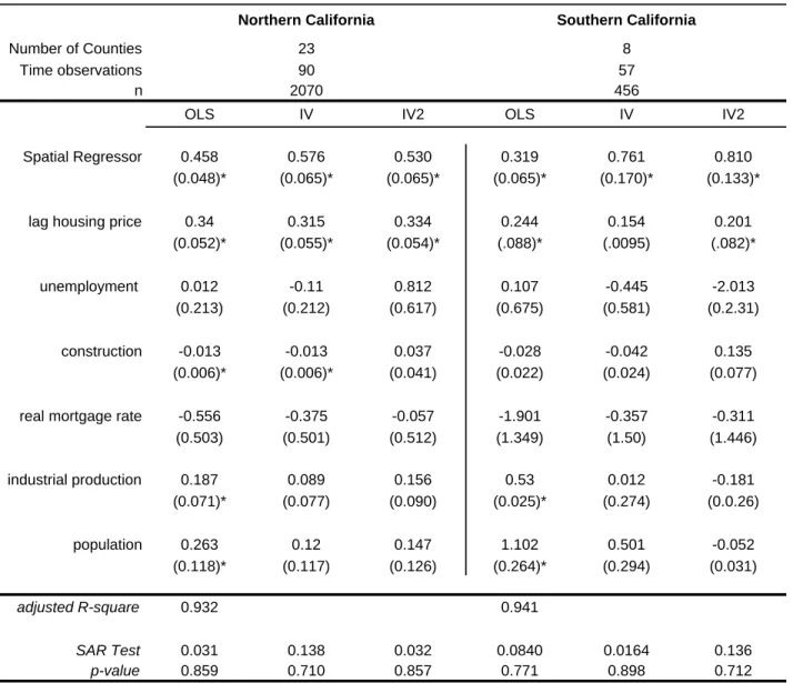
To check the robustness of the model across different time and space, I estimate equation (1) over four samples, delineated by both the constraints of the data set and by geographical interest.16
Given variation in how far back the data extend for each county, the first two samples tested are as follows:
• Sample 1 contains all 31 counties in the sample from April 1998 through December 2002.
• Sample 2 contains 30 counties from July 1995 through December 2002 (San Luis Obispo drops out from Sample 1).
With geography specifically in mind, two additional samples are defined as Northern and South-ern California. These samples are,
• The Northern California sample contains 23 counties from July 1995 through December 2002.
• The Southern California samples contains 8 counties from April 1998 through December 2002.
3.2
Identi
fi
cation
For consistent estimation with a short panel, it would be necessary to control for endogeneity. As example of this, for the endogenous spatial regressor I use the instruments suggested by the spatial literature in addition to the time t−1 lag of the spatial regressor as an instrument. For
1 5
The 31 counties are Alameda, Conta Costa, El Dorado, Fresno, Kern, Los Angeles, Madera, Marin, Merced, Monterey, Napa, Nevada, Orange, Placer, Riverside, Sacramento, San Benito, San Diego, San Francisco, San Joaquin, San Luis Obispo, San Mateo, Santa Barbara, Santa Clara, Santa Cruz, Solano, Sonoma, Stanislaus, Tulare, Ventura, and Yolo.
1 6Data on some counties go back to 1991, allowing for additional samples. However these samples are limited by a lack of contiguity and were not that useful for estimation in this paper.
county unemployment and construction, I first assume both are exogenous. There is evidence in the housing literature suggesting that home construction, at least, is price inelastic in the short run (see Glaeser, Gyourko and Saks (2005), for example). However, lacking stronger evidence, I perform additional IV estimation using the time t−1 lags of construction and unemployment as instruments (in addition to the instruments mentioned for the spatial lag). For the remaining variables, I assume that county population does not respond to housing prices in the current period, and I assume that county housing prices do not effect the aggregate variables, industrial production and the real mortgage rate, in period t. Similar assumptions are found in regional studies by Fratantoni and Schuh (2003) and Carlino and Defina (1998, 1999).
3.3
Baseline Results for the Spatial Model
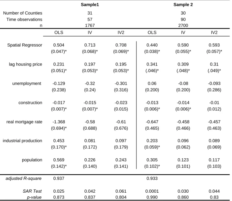
Tables 1 and 2 display results from estimating with OLS and TSLS (for brevity, the tables do not report the results for the dummy variables). The columns labeled IV report the results assuming only the spatial regressor is endogenous, and the columns labeled IV2 report results assuming construction and unemployment, in addition to the spatial regressor, are endogenous.17 Also reported in each table are SAR test statistics for each model, which suggests the spatial correlation is not a feature of the residuals.18 Also, tests for time series autocorrelation in panel data (recommended by Wooldridge (2002)) indicate autocorrelation is not evident in any of the samples.19 Heteroskedasticity-corrected standard errors are reported for each regression.
1 7Results for the Wu-Hausman F test and the Durbin-Wu-Hausman Chi-square tests of the endogeniety of both construction and unemployment suggest the OLS estimation is consistent (or the endogeneity of the regressors does not affect the consistency of OLS). I reject the null hypothesis on both tests for the endogeniety of the spatial regressor, suggesting instrumental variables is needed in each sample.
1 8
The SAR test, an LM statistic (distributedχ2(1)), checks whether the inclusion of the spatial regressor eliminates spatial correlation in the residuals; for each sample I fail to reject the null hypothesis that the residuals are not spatially correlated. Note that before the spatial autoregressive model is estimated, an initial step is to check the residuals of an OLS regression omitting the spatial regressor. Using a common likelihood ratio test from the spatial literature (distributedχ2(1)), I easily reject the null hypothesis for each sample that the residuals are not spatially correlated (where the likelihoods of the OLS model and the spatial error model are compared). The results of the likelihood test suggests the need for the spatial regressor, and the SAR test suggests its inclusion eliminates the spatial correlation from the errors. See Lesage (1999) for details of the likelihood test and other test statistics used in the spatial literature.
1 9
See Wooldridge (2002, page 282). If the lag of the dependent variable is not included in the model, autocorrelation is present in the residuals. The inclusion of the lag in the model eliminates the problem.
Overall, based on the OLS results for each sample reported in Tables 1 and 2, the data support the general findings from spatial housing studies, that conditions in and across regions (and over time) matter for explaining housing prices. In all four samples, the spatial regressor and the time lag of the dependent variable are statistically significant at the five percent level (except for the mortgage rate and the unemployment rate each variable is expressed as a natural log and multiplied by 100, so these coefficients are interpreted as percentages). County population is statistically significant in each sample while unemployment is not significant for any of the samples. County construction is statistically significant in all but the Southern California sample. Industrial production is also statistically significant in each sample while the mortgage rate is significant in only one of the four samples.
For the TSLS estimation, both the lag of the average housing price and the spatial regressor are statistically significant at the five percent level. For the instrumented spatial regressor in both the IV and IV2 regressions, the magnitude of the coefficient is larger relative to the OLS estimation in each sample.20 Also, the remaining explanatory variables are for the most part less precisely estimated and statistically insignificant. Only county construction remains statistically significant in the IV estimation (where it is assumed exogenous), but this is not the case in the IV2 regression, where the instrument for construction is not statistically significant.
Again the IV results are reported to demonstrate how one might proceed from a single-equation dynamic panel model to estimating impulse response functions. If one is interested in estimating structural relationships, as is often the case, then it becomes necessary to employ instrumental variables to identify structural impulse response functions, just as one would need to control for simultaneity when estimating structural impulse response functions from a VAR. The next section reports the impulse responses from applying the linear projections to the spatial model.
2 0First stage F-tests confirm that the endogenous spatial regression is explained by the instruments (the null is easily rejected at the one percent level). However, note that with the typical instruments from the spatial literature, the Hansen J test of over-identifying restriction is rejected, suggesting these instruments may not be appropriate. The overidentifying test of an instrument set with additional time lags of the county regressors (and excluding the spatial “lags”) is not rejected. The IV results turned out to be nearly identical with either instrument set, so I just report the version common to the spatial literature.
One final note on the dynamic panel-spatial model is that I assume a very simple lag structure for the dynamic model. One might prefer a less restrictive model with additional lags of county construction or any of the additional regressors (as one might do when specifying a VAR). However, including additional lags (up to four) for the county and national regressors does not change the qualitative inference of the results reported in the next section, so we focus on equation (4). Also, using the equation estimated with instrumental variables did not produce vastly different impulse response functions (though in the initial periods the linear projection coefficients are larger). For brevity, I only report the impulse response functions for each sample estimated with OLS, where the impulse response functions are constructed by estimating equation (4) h times for the dependent variable,yt+h.
3.4
The Spatial Impulse Response Functions
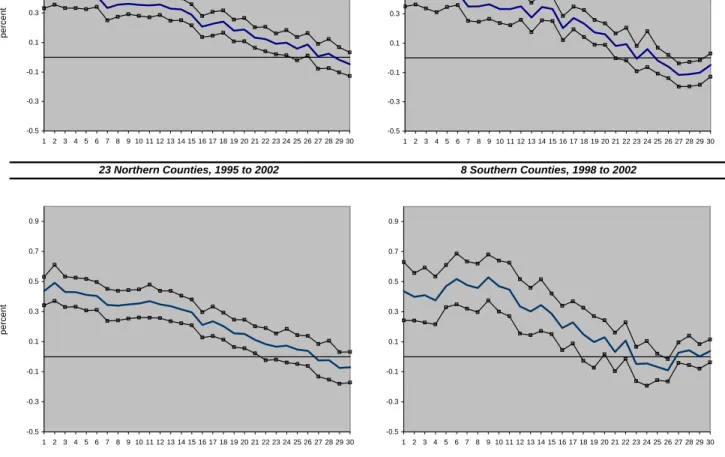
Figure 1 displays the impulse response functions for each of the samples for up to two and half years after a one percent shock to the spatial regressor. Also reported are the plus and minus two-standard error bands, which are constructed from the standard error for the coefficient on the spatial regressor at each horizon. The responses of the dependent variable reveal a consistent picture across the samples. The effect of a change in surrounding regions persists for almost a year at approximately 0.40 percent and remains above zero for at least another year (that is, average housing prices increase by almost half of a percent following the shock). At approximately 25 to 30 months in each of the sample, the impulse response reaches zero. The responses for the three samples with 23 counties or more offer a very similar picture for the diffusion across counties over the horizon. Moreover, the responses are statistically significant at the five percent level for up to two years. The one exception is the response for the Southern California sample, which is statistically significant at the five percent level for up to about seventeen months. However, on balance, these responses reveal that the diffusion of a change in housing prices across regions has a lasting effect over time.
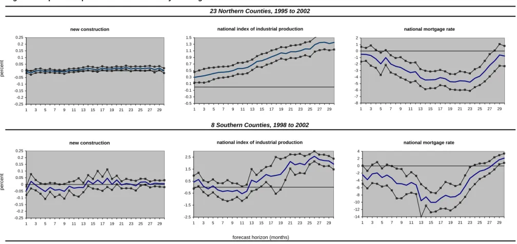
prices to a one percent shock to the real mortgage rate, the index of industrial production and new construction (since the unemployment rate is statistically insignificant in each sample as shown in Tables 1 and 2, I do not report the dependent variable’s response to that regressor). In response to a shock to the real mortgage rate, across the samples, housing prices decline and reach a trough between approximately one and two years after the shock, then return to zero just short of 30 months. The responses are similar expect for the Southern California sample which shows an exaggerated decline relative to the other samples. Housing prices, however, are not responsive to a shock to new construction. This view offers a complementary perspective to the generalfinding in the housing literature that new construction is inelastic with respect to a change in housing prices. On the other hand, regional housing prices do respond to a shock to national industrial production, with the response above zero and statistically significant at the five percent level well up to and past the forecast horizon displayed (though with a delayed effect in the smaller samples).
3.5
Remarks
Overall, Figures 1 through 3 provide a novel picture on the dynamics of regional housing prices across both space and time. Figures 2 and 3 display the response of regional housing prices that are comparable to impulse response functions that could be generated from a time series model; for example, analogous to the VAR estimation in studies by Fratantoni and Schuh (2003) and Pollakowski and Ray (1997). However, as noted by Fratantoni and Schuh (2003), ignoring conditions within regional housing markets leads to misleading estimates of typical, VAR-generated impulse response functions. Hence, unlike previous housing studies, the responses of regional housing prices in this paper are calculated from a model that not only controls for conditions within regions, but also controls for the spatial connection across regions. In other words, the spatial impulse response functions provide a way to control for spatial correlation in order to better understand the effect of shocks on housing prices over time.
Lastly, the spatial impulse functions displayed in Figure 1 provide an additional dimension from which to understand regional dynamics. The response of county housing prices provides a picture
of how a shock to housing prices spreads across regions over time. This view is useful if one is interested in how the spatial correlation between regions will transmit, to what degree and for how long, a shock to housing prices to surrounding regions.
4
Conclusion
In this paper, I apply Jordà’s (2005) linear projection technique to a singe-equation dynamic panel-spatial model. This application provides impulse response functions of housing prices controlling for spatial correlation across California counties, and also shows how a shock to housing prices is transmitted through the spatial correlation over time. This provides a perspective that is difficult to obtain from standard time series techniques (such as with a VAR), or from typical spatial regression analysis. The results in this paper may be of interest to not only those interested in housing markets but those interested in spatial effects more generally.
In addition to the results for housing prices, the approach in this paper suggests a couple of extensions. First, this paper relies on two-stage least squares to estimate the dynamic panel-spatial model. This is admittedly a pragmatic approach as there is not as of yet a direct GMM estimator for spatial models with a dynamic panel. Given the benefits that research on the properties of spatial model estimators has already reaped (see again Kelejian and Prucha (2002), Kapoor, Kelejian and Prucha (2007) and Lee (2003)), a worthwhile direction might be to extend such efforts to spatial dynamic panels. The ability to calculate spatial impulse response functions with Jordà’s (2005) linear projections from spatial dynamic panels suggests such an estimator could be used in other applications. And second, Jordà’s (2005) linear projections need not only apply to spatial models, but can be applied to broader dynamic panel models in a manner similar to the application in this paper.
References
[1] Anselin, Luc,Spatial Econometrics: Methods and Models, Dordrecht, the Netherlands: Kluwer, (1988).
[2] Anselin, Luc, “Spatial Econometrics,” inA companion to Theoretical Econometrics, B.H. Bal-tagi (ed.), Malden: Blackwell, (2001), 310-330.
[3] Anselin, Luc, and Anil K. Bera, “Spatial Dependence in Linear Regression Models with an Introduction to Spatial Econometrics,” in Handbook of Applied Economic Statistics, Aman Ullah and David E.A. Giles (eds.), New York, Marcel Drekker, (1998), 237-289.
[4] Anselin, Luc, and Oleg Smirnov, “Efficient Algorithms for Constructing proper higher order Spatial Lag Operators,”Journal of Regional Science, 36 ,1 (1996) , 67—89.
[5] Arellano, Manuel, Panel Data Econometrics, Oxford University Press, New York (2003). [6] Arellano, M., and S. Bond, “Some Tests of Specification for Panel Data: Monte Carlo Evidence
and an Application to Employment Equations,” Review of Economic Studies, 58, 2, (1991), 277-97.
[7] Arellano, M., and O. Bover, “Another look at the instrumental variable estimation of error-components models,” Journal of Econometrics,68, 1, (July 1995), 29-51.
[8] Badinger, H., Muller, W.G., and G.Tondl, “Regional Convergence in the European Union, 1985-1999: A Spatial Dynamic Panel Analysis,”Regional Studies, 38,3 (2004), 241-253. [9] Basu, S., and T.G.Thibodeau, “Analysis of Spatial Autocorrelation in House Prices,” Journal
of Real Estate Finance and Economics, 17, 1 (1998), 61-85.
[10] Carlino, Gerald, A., and Robert H. Defina, “The Differential Regional Effects of Monetary Policy,”The Review of Economics and Statistics, 80, (1998), 572-587.
[11] Carlino, Gerald, A., and Robert H. Defina, “Do States Respond Differently to Changes in Monetary Policy,” Business Review, (July/August 1999), 17-27.
[12] Case, Anne, C., “Spatial Patterns in Household Demand,”Econometrica, 59, (1991), 953-965. [13] Case, Karl E. and Robert J. Shiller, “Is There a Bubble in the Housing Market?” Brookings
Papers on Economic Activity, no.2 (2003), 299-341.
[14] Clapp, John, M., and Dogan Tirtiroglu, “Positive Feedback Trading and Diffusion of Asset Price Changes: Evidence from Housing Transactions,” Journal of Economic Behavior and Organization, 24, (1994), 337-355.
[15] Elhorst, Paul, J., “Specification and Estimation of Spatial Panel Data Models,”International Regional Science Review, 26,3 (July 2003), 244-268.
[16] Fratantoni, Michael, and Scott Schuh, “Monetary Policy, Housing, and Heterogeneous Regional Markets,”Journal of Money, Credit and Banking, 35,4 (August 2003), 557-589.
[17] Glaeser, E.L., Gyourko, J., and R.E. Saks, “Why Have Housing Prices Gone Up?” American Economic Review, 95, 2, (May 2005), 329-333.
[18] Holly, S., Pesaran, M. H., and T. Yamagata, “A Spatio-Temporal Model of House Prices in the U.S.,”University of Cambridge Working Paper, (April 2007).
[19] Hoover, Kevin, S., and Òscar Jordà, “Measuring systematic monetary policy,”Review, Federal Reserve Bank of St. Louis, (July 2001), 113-144.
[20] Hsiao, C.,Analysis of Panel Data, 2nd edition, Cambridge, UK, Cambridge University Press (2003).
[21] Hwang, M., and J.M. Quigley, “Economic Fundamentals in Local Housing Markets: Evidence from U.S. Metropolitan Regions,”Journal of Regional Science, 46, 3 (2006), 425—453.
[22] Jordà, Òscar, “Estimation and Inferences of Impulse Responses by Local Projections,” Amer-ican Economic Review, 95:1 (2005), 161-182.
[23] Jordà, Òscar, “Simultaneous Confidence Regions for Impulse Responses”Review of Economics and Statistics, forthcoming (2007).
[24] Jordà, Òscar, and Sharon Kozicki, “Estimation and Inference by the Method of Projection Minimum Distance,”UC Davis Working Paper (2007).
[25] Kapoor,M., Kelejian, H. H., and I. Prucha„ “Panel Data Models with Spatially Correlated Error Components”Journal of Econometrics,140, (2007), 97—130.
[26] Kelejian, H. H., and I. Prucha, “2SLS and OLS in a Spatial Autoregressive Model with Equal Weights,”Journal of Regional Science and Urban Economics 32, (2002), 691-707.
[27] Kelejian, H. H., and D.P. Robinson, “A suggested method of estimation for spatial interdepen-dent models with autocorrelated errors, and an application to a county expenditure model,”
Papers in Regional Science, 72, 3 (July 1993), 297-312.
[28] Krainer, J., “Housing Markets and Demographics,” FRBSFEconomic Letter,2005-21 (August 2005).
[29] Krainer, J., and C. Wei, “House Prices and Fundamental Value,” FRBSF Economic Letter,
2004-27 (October 2004).
[30] Lee, Lung-fei, “Best Spatial Two-Stage Least Squares Estimators for a Spatial Autoregressive Model with Autoregressive Disturbances,”Econometric Reviews, 22, 4, (January 2003), 307 -335.
[31] LeSage, James P., The Theory and Practice of Spatial Econometrics, University of Toledo, unpublished book, February 1999.
[32] McCarthy, Jonathan, and Peach, Richard W., “Monetary Policy Transmission to Residential Investment,” Economic Policy Review, 8,1 (May 2002).
[33] Pollakowski, Henry, O., and Traci S. Ray, “Housing Price Diffusion Patterns at Different Aggre-gation Levels: An Examination of Housing Market Efficiency,” Journal of Housing Research, 8, 1 (1997), 107-124.
[34] Stock, J., and M. Watson, “Vector Autoregressions,” Journal of Economic Perspectives, 15, 4 (Fall 2001), 101-115.
[35] Tirtiroglu, Dogan, “Efficiency in Housing Markets: Temporal and Spatial Dimensions,” Jour-nal of Housing Economics, 2, 3, (1992), 276-292.
[36] Varga, Attila, “Local Academic Knowledge Transfers and the Concentration of Economic Activity,”Journal of Regional Science, 40, 2 (May 2000), 289-309.
[37] Wooldridge, Jeffrey, M.,Econometric Analysis of Cross Section and Panel Data, MIT Press, Cambridge, Massachusetts (2002).
Number of Counties Time observations n
OLS IV IV2 OLS IV IV2
Spatial Regressor 0.504 0.713 0.708 0.440 0.590 0.593
(0.047)* (0.068)* (0.069)* (0.038)* (0.055)* (0.057)*
lag housing price 0.231 0.197 0.195 0.341 0.309 0.31
(0.051)* (0.053)* (0.053)* (.046)* (.048)* (.049)*
unemployment -0.129 -0.32 -0.301 0.06 -0.08 -0.093
(0.238) (0.24) (0.316) (0.200) (0.200) (0.286)
construction -0.017 -0.015 -0.023 -0.013 -0.014 -0.01
(0.007)* (0.007)* (0.015) (0.006)* (0.006)* (0.012)
real mortgage rate -1.368 -0.58 -0.61 -0.647 -0.458 -0.457
(0.694)* (0.688) (0.676) (0.465) (0.466) (0.463) industrial production 0.453 0.081 0.097 0.203 0.096 0.089 (0.170)* (0.172) (0.179) (0.059)* (0.062) (0.069) population 0.569 0.226 0.243 0.305 0.123 0.117 (0.142)* (0.140) (0.141) (0.102)* (0.101) (0.103) adjusted R-square 0.937 0.933 SAR Test 0.025 0.042 0.061 0.0001 0.030 0.044 p-value 0.873 0.837 0.804 0.990 0.860 0.83 2700
Notes: The results displayed are for ordinary least squares and two-stage least squares estimation. For columns labeled IV, the instrument set for the endogenous spatial regressor includes the spatial lags of unemployment, construction, county population and the spatial regressor lagged one period. For IV2, with the endogenous spatial regressor, unemployment and construction, the instrument includes one period lags of unemployment and
construction (in addition to the spatial lags). First stage F-tests for each endogenous regressor are easily rejected at the five percent level (not shown). Heteroskedasticity-corrected standard errors are shown in the parentheses. Tests for autocorrelation in panel data (recommended by Wooldridge (2002)) indicate autocorrelation is not evident in any of the samples (not shown). The null of the SAR test is that spatial correlation is not evident in the residuals. The SAR is a Lagrange multiplier statistic and is distributed Χ²(1). *Indicates the coefficient estimate is significant at the five percent level.
Table 1: Estimates for the Dynamic Panel-Spatial Model
Sample 2 30 90 Sample1 31 57 1767
Number of Counties Time observations n
OLS IV IV2 OLS IV IV2
Spatial Regressor 0.458 0.576 0.530 0.319 0.761 0.810
(0.048)* (0.065)* (0.065)* (0.065)* (0.170)* (0.133)*
lag housing price 0.34 0.315 0.334 0.244 0.154 0.201
(0.052)* (0.055)* (0.054)* (.088)* (.0095) (.082)*
unemployment 0.012 -0.11 0.812 0.107 -0.445 -2.013
(0.213) (0.212) (0.617) (0.675) (0.581) (0.2.31)
construction -0.013 -0.013 0.037 -0.028 -0.042 0.135
(0.006)* (0.006)* (0.041) (0.022) (0.024) (0.077)
real mortgage rate -0.556 -0.375 -0.057 -1.901 -0.357 -0.311
(0.503) (0.501) (0.512) (1.349) (1.50) (1.446) industrial production 0.187 0.089 0.156 0.53 0.012 -0.181 (0.071)* (0.077) (0.090) (0.025)* (0.274) (0.0.26) population 0.263 0.12 0.147 1.102 0.501 -0.052 (0.118)* (0.117) (0.126) (0.264)* (0.294) (0.031) adjusted R-square 0.932 0.941 SAR Test 0.031 0.138 0.032 0.0840 0.0164 0.136 p-value 0.859 0.710 0.857 0.771 0.898 0.712
Table 2: Estimates for the Dynamic Panel-Spatial Model: Alternative Samples
Notes: See Table 1 comments.
Southern California 8 57 456 Northern California 23 90 2070
Notes: The impulse response functions are estimated with Jordà's (2005) linear projection technique; these are calculated from a dynamic panel-spatial model estimated with OLS (and controlling for fixed effects with dummy variables). The solid line represents the function, while the surrounding bands are the plus or minus 2-standard error bands.
forecast horizon (months)
Figure 1: Impulse Response Functions of County Housing Prices to a shock to the Spatial Regressor
percent
percent
30 Counties, 1995 to 2002 31 Counties, 1998 to 2002
23 Northern Counties, 1995 to 2002 8 Southern Counties, 1998 to 2002
-0.5 -0.3 -0.1 0.1 0.3 0.5 0.7 0.9 1 2 3 4 5 6 7 8 9 10 11 12 13 14 15 16 17 18 19 20 21 22 23 24 25 26 27 28 29 30 -0.5 -0.3 -0.1 0.1 0.3 0.5 0.7 0.9 1 2 3 4 5 6 7 8 9 10 11 12 13 14 15 16 17 18 19 20 21 22 23 24 25 26 27 28 29 30 -0.5 -0.3 -0.1 0.1 0.3 0.5 0.7 0.9 1 2 3 4 5 6 7 8 9 10 11 12 13 14 15 16 17 18 19 20 21 22 23 24 25 26 27 28 29 30 -0.5 -0.3 -0.1 0.1 0.3 0.5 0.7 0.9 1 2 3 4 5 6 7 8 9 10 11 12 13 14 15 16 17 18 19 20 21 22 23 24 25 26 27 28 29 30
forecast horizon (months)
Notes: See Figure 1. The figures show the response of average county housing prices to additional regressors in the dynamic panel-spatial model. See text for details.
30 Counties, 1995 to 2002
31 Counties, 1998 to 2002 Figure 2: Impulse Response Functions of County Housing Prices to additional Factors
percent percent new construction -0.25 -0.2 -0.15 -0.1 -0.05 0 0.05 0.1 0.15 0.2 0.25 1 3 5 7 9 11 13 15 17 19 21 23 25 27 29
national index of industrial production
-0.5 -0.3 -0.1 0.1 0.3 0.5 0.7 0.9 1.1 1.3 1.5 1 3 5 7 9 11 13 15 17 19 21 23 25 27 29
national mortgage rate
-8 -7 -6 -5 -4 -3 -2 -1 0 1 2 1 3 5 7 9 11 13 15 17 19 21 23 25 27 29 new construction -0.25 -0.2 -0.15 -0.1 -0.05 0 0.05 0.1 0.15 0.2 0.25 1 3 5 7 9 11 13 15 17 19 21 23 25 27 29
national index of industrial production
-2.5 -1.5 -0.5 0.5 1.5 2.5 1 3 5 7 9 11 13 15 17 19 21 23 25 27 29
national mortgage rate
-8 -6 -4 -2 0 2 4 1 3 5 7 9 11 13 15 17 19 21 23 25 27 29
23 Northern Counties, 1995 to 2002
8 Southern Counties, 1998 to 2002
Figure 3: Impulse Response Functions of County Housing Prices to additional Factors: Northern and Southern California
percent
percent
forecast horizon (months) Notes: See Figures 1 and 2.
new construction -0.25 -0.2 -0.15 -0.1 -0.05 0 0.05 0.1 0.15 0.2 0.25 1 3 5 7 9 11 13 15 17 19 21 23 25 27 29
national index of industrial production
-0.5 -0.3 -0.1 0.1 0.3 0.5 0.7 0.9 1.1 1.3 1.5 1 3 5 7 9 11 13 15 17 19 21 23 25 27 29
national mortgage rate
-8 -7 -6 -5 -4 -3 -2 -1 0 1 2 1 3 5 7 9 11 13 15 17 19 21 23 25 27 29 new construction -0.25 -0.2 -0.15 -0.1 -0.05 0 0.05 0.1 0.15 0.2 0.25 1 3 5 7 9 11 13 15 17 19 21 23 25 27 29
national index of industrial production
-2.5 -1.5 -0.5 0.5 1.5 2.5 1 3 5 7 9 11 13 15 17 19 21 23 25 27 29
national mortgage rate
-14 -12 -10 -8 -6 -4 -2 0 2 4 1 3 5 7 9 11 13 15 17 19 21 23 25 27 29