Air Force Institute of Technology
AFIT Scholar
Theses and Dissertations Student Graduate Works
3-26-2015
A Predictive Logistic Regression Model of World
Conflict Using Open Source Data
Benjamin C. Boekestein
Follow this and additional works at:https://scholar.afit.edu/etd
This Thesis is brought to you for free and open access by the Student Graduate Works at AFIT Scholar. It has been accepted for inclusion in Theses and
Recommended Citation
Boekestein, Benjamin C., "A Predictive Logistic Regression Model of World Conflict Using Open Source Data" (2015).Theses and Dissertations. 101.
The views expressed in this thesis are those of the author and do not reflect the official policy or position of the Department of the Army, Department of Defense, or the United States Government. This material is declared a work of the U.S. Government and is not subject to copyright protection in the United States.
AFIT-ENS-MS-15-M-112
A PREDICTIVE LOGISTIC REGRESSION MODEL OF WORLD CONFLICT USING OPEN SOURCE DATA
THESIS
Presented to the Faculty Department of Operational Sciences Graduate School of Engineering and Management
Air Force Institute of Technology Air University
Air Education and Training Command In Partial Fulfillment of the Requirements for the Degree of Master of Science in Operations Research
Benjamin C. Boekestein, BS MAJ, USA
March 2015
DISTRIBUTION STATEMENT A.
AFIT-ENS-MS-15-M-112
A PREDICTIVE LOGISTIC REGRESSION MODEL OF WORLD CONFLICT USING OPEN SOURCE DATA
THESIS Benjamin C. Boekestein, BS MAJ, USA Committee Membership: Dr D. K. Ahner Chair Dr. R. F. Deckro Member
AFIT-ENS-MS-15-M-112
Abstract
Nations transitioning into conflict is an issue of national interest. This study considers various data for inclusion in a statistical model that predicts the future state of the world where nations will either be in a state of “violent conflict” or “not in violent conflict” based on available historical data. Logistic regression is used to construct and test various models to produce a parsimonious world model with 15 variables. Open source data for the previous year is not immediately available for predicting the following year, so an approach is developed that ensures only historical data that would be available for such a prediction is used. Further analysis shows that nations differ significantly by geographical area. Therefore six sub-models are constructed for differing geographical areas of the world. The dominant variables for each sub-model vary, suggesting a
complex world that cannot be modeled as a whole. Insights and conclusions are gathered from the models, a best model is proposed, and predictions are made for the state of the world in 2015. Accuracy of predictions via validation surpass 80%. Eighty-five nations are predicted to be in a state of violent conflict in 2015, seventeen of them are new to conflict since the last published list in 2013. A prediction tool is created to allow war-game subject matter experts and students to identify future predicted violent conflict and the responsible variables.
Dedication
This work is dedicated to my wife and our four children. They are my inspiration and my joy.
Acknowledgments
I would like to express my deep gratitude to my advisor, Dr. K. Darryl Ahner for his direction, support and mentorship during my research. I wish to thank Dr. Richard K Deckro for his insights and contributions.
Table of Contents
Page
Abstract ... iv
Table of Contents ... vii
List of Figures ... ix List of Tables ... xi I. Introduction ...1 General Issue ...1 Problem Statement...1 Research Objectives/Questions/Hypotheses ...1 Research Focus ...2 Research Questions ...2 Methodology...2 Assumptions/Limitations ...2 Implications ...3 Overview ...4
II. Literature Review ...5
Relevant Research ...5
III. Methodology ...13
Chapter Overview ...13
Method to Select the nations to Model ...26
Method to Select the Dependent Variable ...26
Method to select and screen independent variables and to impute missing data ...29
IV. Analysis and Results ...46
Chapter Overview ...46
Results of Constructing Logistic Regression Trial Models ...46
Factor Analysis and Noise Reduction Techniques ...57
Initial Sensitivity Analysis ...67
Analysis using an expanded database...71
Separate Models for Six Regions ...80
Sensitivity Analysis on the study’s best model ...83
Methods to Predict Nations not currently in Violent Conflict transitioning to Violent Conflict ...86
Forecasting the Future: 2014 ...90
Forecasting the Future: 2015 ...92
Investigative Questions Answered ...94
Summary...95
V. Conclusions and Recommendations ...96
Conclusions of Research ...96
Significance of Research ...96
Recommendations for Action ...96
Recommendations for Future Research...97
Appendix A: List of nations in each region ...98
Appendix B: Story Board...99
List of Figures
Page
Figure 1: Linear and Logistic Functions ... 15
Figure 2: Conditions for the Likelihood Ratio R Square ... 21
Figure 3: Conditions for the Un-Adjusted Geometric Mean R Square ... 21
Figure 4: Conditions for the Adjusted Geometric Mean R Square ... 22
Figure 5: Conditions for Hosmer Lemenshow... 23
Figure 6: Confusion Matrix ... 24
Figure 7: Logistic Regression Test for Significance ... 25
Figure 8: Effect Likelihood Ratio Test ... 25
Figure 9: Trial Model 1 Output ... 47
Figure 10: Trial Model 2 Output ... 48
Figure 11: Trial Model 3 ... 49
Figure 12: Trial Model 4 ... 50
Figure 13: Signal to Noise Ratio, Trial Model 5 & 6 ... 51
Figure 14: Trial Models 5 & 6 ... 52
Figure 15: Trial Models 7, 8 & 9 ... 53
Figure 16: Signal to Noise Ratio, Trial Model 7 & 8 ... 53
Figure 17: Signal to Noise Ratio, Trial Model 9 ... 54
Figure 18: Trial Model 7 Test Set Prediction Accuracy ... 57
Figure 19: Scree Plot and Horn's Curve ... 58
Figure 22: Harshness of Life vs Political Oppression Lower Left Quadrant ... 63
Figure 23: Harshness of Life vs Factor 4 Lower Left Quadrant ... 64
Figure 24: Political Oppression vs Trade & Population Density Upper Left Quadrant .. 65
Figure 25: Trial Model 10 and Trial Model 11 ... 66
Figure 26: Confusion matrix results when adjusting the cut off value ... 69
Figure 27: Confusion Matrices Excluding Nations in Conflict by Choice ... 71
Figure 28: Trial Model 7 Applied to Expanded Database ... 73
Figure 29: Expanded Database ... 75
Figure 30: Trial Model 12 by Regions ... 76
Figure 31: Region Groups ... 77
Figure 32: Model with Region Variable ... 78
Figure 33: Trial Model 13 by Region ... 79
Figure 34: Trial Model 14 - Separate Region Models ... 80
Figure 35: Individual Models... 82
Figure 36: Prediction Accuracies ... 83
Figure 37: Trial Model 14, Cutoff of .28 ... 85
Figure 38: Method 2 Confusion Matrix ... 87
Figure 39: 2014 Predictions ... 91
List of Tables
Page
Table 1: HIIK Conflict Items ... 28
Table 2: HIIK Intensity Level and Level of Violence ... 29
Table 3: HIIK Intensity Level Scoring Method ... 29
Table 4: Country Statistic Variables ... 31
Table 5: Conflict in Bordering States Calculation ... 32
Table 6: Regime Type ... 34
Table 7: 2 yr HIIK Trend Formula and Example ... 36
Table 8: VIF Values for 26 Variables ... 37
Table 9: VIF Values for 23 Variables ... 39
Table 10: Correlation Heat Map before Removing Variables ... 40
Table 11: Correlation Heat Map after Removing Variables ... 40
Table 12: Number of Variables per Nation; Nations with Worst Data ... 41
Table 13: Correlation with HIIK Intensity Level ... 43
Table 14: Trial Model Prediction Accuracy ... 55
Table 15: Coefficients for Trial Model 7 ... 56
Table 17: Factor Loadings and Variance Explained ... 59
Table 18: New Prediction Accuracy ... 67
Table 19: List of Extreme False Positives and False Negatives ... 70
Table 22: Mathematical Likelihood of False Negatives ... 88 Table 23: Historical probability of False Negatives ... 89
A PREDICTIVE LOGISTIC REGRESSION MODEL OF WORLD CONFLICT USING OPEN SOURCE DATA
I. Introduction
General Issue
The value of knowing the future state of the world is priceless. Numerous
government agencies and civilian companies produce models to predict the future state of the world. Gaining information about the future gives these organizations a decided advantage in preparation and planning for future events. Models have the potential to offer valuable insights when applied correctly. The renowned statistician and often quoted George Box said “Essentially, all models are wrong, but some are useful” (Box, 1979). No model will ever accurately predict the future, but some models can offer useful insights and give greater clarity to decision makers. This study develops a model that predicts violent conflict in the world using logistic regression and open source data.
Problem Statement
This study develops a suite of models to predict nations that are in a state of violent conflict using a logistic regression model and open source data. These models are used to predict nations in a violent conflict in 2015.
Research Objectives/Questions/Hypotheses
The objectives of this study are to predict future violent conflict in the world and to identify variables that contribute significantly to violent conflict.
Research Focus
This study focuses on logistic regression as the modeling method to predict violent conflict. The years analyzed include 2008 through 2013.
Research Questions
How accurately can a Logistic Regression Model predict the state of the world; can it identify nations that will be in a state of “violent conflict” and nations that will not?
Are there key variables from open source data that contribute to a predictive model of nation conflict?
Given a nation is falsely predicted to be in a violent conflict, how likely is it to enter into a violent conflict the following year or within 2-4 years?
Methodology
Logistic regression is used to construct the models. Three different logistic regression model building techniques are introduced and used in this study. The method to construct the dependent variable is discussed as well as methods to build, screen, and test independent variables.
Assumptions/Limitations
This study assumes that there are variables that contribute to a nation being in a violent conflict and can be used as predictors of violent conflict. It also assumes these predictors remain relevant from year to year. The study assumes that the variable data is accurate and collected in a consistent manner and demonstrates causation of the
The model is limited by data availability, which mandated a two and three year lag on all of the variables. A model built off of previous year data would be superior to the models in this study but would not answer the study problem. It would serve no purpose to develop a model that accurately predicts 2014 when it is already 2014. At the time this study was conducted, in 2014, most of the data sets were complete up through 2012 and sometimes 2013. To predict into the future, in this case 2015, the model has to rely on two and three year old data. “Black Swan” events, such as Al Qaeda detonating a VBIED on the Golden Mosque and spiraling Iraq into a civil war are nearly
unpredictable. This study cannot account for “Black Swan” events. The study was limited by availability of the dependent variable. The Heidelberg Institute for Conflict Research was updating their database and was unable to provide data for this study. The data was collected through AFIT analysis of Heidelberg Institute for Conflict Research pdf documents. The models produced in this study do not accurately predict previously stable nations that enter into a violent conflict by choice. These nations’ actions do not typically depend on the factors that lead to violent conflict in less stable nations.
Implications
The recommended model from this study could lend insight into nations that are strong candidates for entering into a violent conflict and nations that are strong
candidates for exiting a violent conflict. The study will also identify variables that are key contributors to violent conflict. Identifying these variables could give decision makers focus for their efforts to improve stability in a nation.
Overview
The study begins with a review of previous. Next, logistic regression is introduced, followed by a description of the dependent and independent variables. Methods to build models are described and then implemented. Sensitivity of the cutoff value that classifies country conflict state is performed. Finally, the study will conclude with analysis of the models, answers to the research questions and conclusions. A list of 2014 and 2015 predictions are presented.
II. Literature Review
The purpose of this chapter is to provide background information for this study. This chapter will discuss relevant research that informs this study, including a CIA task force study, several Center for Army Analysis (CAA) instability studies and various other indices of instability. The single most influential document for this study is the FACT study conducted by Robert Shearer and analysts from the Center for Army Analysis.
Relevant Research
Numerous previous studies predict instability in nations. Researchers in the Central Intelligence Agency’s State Failure Task Force investigated several methods to predict political instability using various methods (logistic regression, neural networks, and Markov models)(Shearer, 2010). The CIA task force achieved over 80% accuracy in predicting instability with a logistic regression model using regime type, infant mortality rate, conflict in bordering states, and state discrimination as predictors(Goldstone, 2005). This CIA funded study used global data from 1955 to 2003. The task force categorized and compiled over 200 major political instability events during this time. The dependent variable was an onset of one of these events, which included Revolutionary Wars, Ethnic Wars, Adverse Regime Changes, and Genocides and Politicides. The task force tested hundreds of independent variables, their interactions and rates of change. This study compiles their own data for the dependent variable, making it very difficult to validate
the model’s accuracy. The CIA study randomly selects nations to validate their model; the claimed 80% accuracy is not a “whole world” accuracy, but a smaller random sample.
The Center for Army Analysis has conducted multiple studies analyzing
instability induced conflict. Three CAA studies are significant. These studies include the Political and Economic Risk in Countries and Lands Evaluations (Ahrens, 1997), the Analysis of Complex Threats studies (Bundy and Mathur, 1997 and O’Brien, 2001a), and the Analysis of Complex Threats for Operations and Readiness study (O’Brien, 2001b). The most accurate model from these studies was a possibility theory model that achieved 90% accuracy in predicting conflict five years into the future. Critics suggested this study was difficult to understand and the results were incomprehensible to staff and senior decision makers.
To produce a more “user-friendly” study the CAA initiated the Forecast and Analysis of Complex Threats (FACT) study in 2007. Shearer and Marvin were the FACT study directors and wrote an article in the Military Operations Research journal
Recognizing Patterns of Nation-State Instability that Lead to Conflict (Marvin, 2010). They built upon the previous studies done at the Center for Army Analysis to accomplish three tasks. First they identify features that capture the instability of a nation, second they forecast the future levels of these features for each nation and third they classified each future state’s conflict potential.
Shearer and Marvin intended to predict the future conflict potential of select nation-states in a simple manner. The study used thirteen unclassified data sets categorized into four of the six PMESII categories; Political, Military, Economic and
The variables are shown below along with their unclassified data source. The data set included the years 1993-2003.
• Political
• Civil liberties – Freedom House
• Democracy – Polity IV Project
• Political rights – Freedom House
• Military
• Conflict history – Heidelberg Institute of Conflict Research
• Economic
• Male unemployment – World Bank
• GDP per capita – World Bank
• Trade openness – World Bank
• Social
• Adult Male literacy – World Bank
• Caloric intake – Food and Agriculture Organization of the United
Nations
• Ethnic diversity – CIA World Fact Book
• Infant mortality – U.S. Bureau of the Census
• Life expectancy – U.S. Bureau of the Census
• Religious diversity – CIA World Fact Book
The conflict history data came from the Heidelberg Institute of Conflict Research(Heidelberg Institute for International Conflict Research, 2014). Conflicts were defined as the clashing of interests on national values and issues and were classified according to amount of violence observed. The four categories were Latent Conflict, Crisis, Severe Crisis and War. Shearer states that historically the United States has not intervened in foreign nations until casualties are experienced so the authors combined the
Crisis)(Shearer, 2010). Different to Sherarer’s study, the 2014 HIIK study categorizes the conflicts into six categories instead of four, as outlined in the methodology section of this paper. Shearer’s study consisted of two important assumptions:
1) Nations that experienced conflict are similar in that they share common
instability features.
2) The distance between the scaled 13 dimension vectors can serve as a
reasonable scale for the similarity between two nation-states.
After the data was collected for each nation Shearer used a visual method to test their assumptions by generating 54 three-dimension plots from each of the possible combinations of 1 political, 1 social and 1 economic/military. Points were colored on historical levels of conflict observed; gray for peace and black for conflict. If the
variables were significant the team expected the points to be grouped in a cloud by color. Most of the 54 plots did not show distinct color groups; a few did. The initial verification method was unsatisfying so a second method was explored. The Principal Component Analysis (PCA) method reduced the 13 variables into three dimensions that could be visually analyzed. The three components were assigned the terms “social”, “political” and “military/economic”. The PCA method searches for linear combinations of the original 13 vectors that best express the variance in the data. Using this method the study graphs distinct conflict (black) and peace (gray) clouds and satisfies the two key
assumptions. Because the FACT study uses Principal Component analysis it does not show causation between independent variables and violent conflict.
Shearer used a weighted moving average to predict future values and divided their data set into a training set (first 6 years) and a test set (last 5 years). To classify the future
data points derived from the weighted moving averages the team used the K-nearest neighbor algorithm and nearest centroid algorithm. The nearest neighbor proved to be more accurate than the centroid algorithm. They used the same portioning of the data to predict (first 5 years) and test (last 6 years) and adjusted the number of neighbors
between 3 and 11. With the nearest neighbor algorithm the team used a simple majority of neighbors to classify their predicted nation status. The K-nearest neighbor, with K=7, performed the best with an 87% accuracy. All the other K-nearest neighbors also
achieved over 85% accuracy. The predicted nation scores were classified as peace, conflict or uncertain with about 25% classified as uncertain. Without the uncertain classification, the study prediction accuracy for their validation set was 76% This study relied on the data from the same year in which the conflict was determined.
The Center for Army Analysis adopted Shearer’s FACT study method which used a weighted average and K-nearest neighbor algorithm. It has comparable accuracies to earlier studies but with predictions further into the future and is easier to understand (Shearer, 2010).
Valuable insight into grouping the nations of the world in explainable groups came from Hans Rosling. Hans Rosling is a renowned statistician, medical doctor and public speaker. He has accumulated numerous accolades with his innovative statistical methods, including being named by Time Magazine as one of the 100 most influential people in 2012(Christakis, 2012). Mr Rosling is a co-founder of the Gapminder
foundation which developed the trendalyzer software system (Gapminder, A fact-based worldview). Mr Rosling has become a prominent public speaker using the trendalyzer
software. In a 2006 “Ted Talks” lecture Rosling divides the world into the following six categories: (The best stats you've ever seen, 2006)
• Organization for Economic Co-operation and Development (OECD) nations
• Latin America nations
• East European nations
• East Asian nations
• South Asian nations
• African nations
Rosling further subdivides the African nations into Sub Saharan African nations and Arab states (includes much of Middle East). These groupings of nations will inform nation groupings in this study. A list of countries in each group is available in Appendix A.
Directly related to countries in conflict is a country’s aptitude to become a failed state. The Fund for Peace provides an index of fragile states in the world (The Fund for Peace , 2015). The fragile states index measures fragile states and ranks them for likelihood of failing. The 2013 fragile state index ranks all countries using 12 variables to determine a final failed state index. These variables include:
• Demographic Pressures
• Refugees and Internally Displaced Persons
• Group Grievance
• Human Flight
• Uneven Development
• Poverty and Economic Decline
• Legitimacy of the State
• Public Service
• Factionalized Elites
• External Intervention
These 12 variables are significant factors for failed states and are also potential factors for predicting violent conflict. The fragile state list provides a separate index to compare the results of this study with.
Open source data for stability models is available from several reputable sources. The study’s independent variables come from four places; the World Bank, CIA World Factbook, Freedom House and the Center for Systemic Peace.
The World Bank was established in 1944, is headquartered in Washington DC and has more than 10,000 employees in more than 120 offices worldwide (World Bank, 2015). This organization has thousands of data sets. The CIA World Factbook provides information on the history, people, government, economy, geography, communications, transportation, military and transnational issues for 267 world entities (Center for Systemic Peace, 2014). Freedom House, established in 1941, is an independent watchdog organization originally created to encourage popular support for American involvement in World War II. In the 1970s Freedom House began to focus on a global view of civil liberties and political rights, publishing its first annual publication “Freedom in the World” in 1973 (Freedom House, 2012). The Freedom House organization
provides nation scores for civil liberties and political rights. The Polity IV project is created by the Center for Systemic Peace (CSP) which is a not-for-profit organization that monitors political behavior in each of the world’s major states. They record data for 167 nations (Center for Systemic Peace, 2014).
The literature review for this study focused on work performed by Robert Shearer, the Center for Army Analysis, and available data sources. A CIA study
provided valuable information on previous logistic regression models and variables that were significant for them. The best CIA model was able to predict with 80% accuracy. Shearer constructed a model that used a K-nearest neighbor algorithm and achieved 76% accuracy over six years.
III. Methodology
Chapter Overview
This chapter discusses the various methods used for this study. The chapter begins with a review of logistic regression; the regression tool used to construct the models in this study. The section on logistic regression includes a summary of logistic regression, a discussion of the logistic regression statistics, and a review of the logistic regression goodness of fit tests. The next section includes the method to select the nations to model followed by a description of the dependent variable. Other discussions include the method to select and screen the independent variables as well as impute missing data. The database used for analysis is discussed as well as a description of the training and test data sets. Three different methods to construct a model are introduced. The chapter finishes with a discussion on methods to analyze only nations that enter into a violent conflict and nations that exit a violent conflict.
Logistic Regression
Before understanding logistic regression it is important to understand why linear regression cannot be applied when dealing with a dichotomous dependent variable. The response for this study is either “in a violent conflict” or “not in a violent conflict”, which is dichotomous. Linear regression is the usual method for predicting a response,
however, linear regression relies on some primary assumptions, listed below, that are unmet with a dichotomous dependent variable.
1. Measurement: All independent variables are interval, ratio, or dichotomous, and the dependent variable is continuous, unbounded, and measured on an interval or ratio scale
2. Specification. All relevant predictors of the dependent variable are included in the analysis
3. Expected value of error. The expected value of the error is 0, or can be transformed to be so.
4. Linearity: Predictors are linearly related to the Dependent Variable
5. Homoscedasticity: Residual variance is constant about the regression surface
6. Normality: of the distribution residuals
7. No autocorrelation among error terms
8. No correlation between the error terms and the independent variables
9. Absence of perfect multicollinearity
(Menard, 2001) When assumptions are violated the model can have serious consequences and lead to wrong conclusions. Transformations are one way to deal with violated assumptions. A number of these assumptions are violated when the dependent variable is dichotomous: Consider the linear equation
i i i
y =x′β ε+
Equation 1: Linear Equation
There are some basic problems with this regression model when using a dichotomous dependent variable. If the response is binary, then the error termsεi can only take on two values, 1 and 0. This means the error terms in this model cannot be normal.
(Montomgery, 2012) Therefore, the Normality assumption is violated. The error variance is not constant, since εi = −yi pi and piis a constant and yi takes on the values of either 1 or 0, therefore εi changes for each i and the homoscedasicity (constant variance) assumption is violated. Not all independent variables for this study are interval,
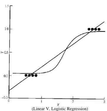
ratio, or dichotomous and the dependent variable is not continuous and it is bounded. Therefore the Measurement assumption is violated. The response is constrained between 0 and 1. A linear function could include values that lie outside this interval, as shown in Figure 1. The logistic regression response in this figure is constrained between 0 and 1 over the interval from 0 to 3 while the linear line is not.
(Linear V. Logistic Regression)
Figure 1: Linear and Logistic Functions
With all the previously stated issues, a linear equation cannot be applied when the dependent variable is dichotomous. A monotonically increasing (or decreasing) S-shaped function is usually employed (Montomgery, 2012). An example of this S shaped function is portrayed in Figure 1, along with a linear function. This nonlinear function has the form shown in Equation 2 and is called the logistic response
1 ( ) 1 1 x x x e E y p e e β β β ′ ′ − ′ = = = + +
Equation 2: Logistic Response Function
If we use the natural logarithm of the dependent variable we no longer face the problem that the estimated probability may exceed the maximum or minimum possible values for the probability. The values will be contained between 0 and 1. If a value is less than .5 it will be rounded to 0 (not in a violent conflict), if a value is greater than or equal to .5 it will be rounded to 1 (in a violent conflict). Figure 1 depicts OLS and a logistic regression for the same data points. The OLS line predicts values lying outside of the allowable range (less than 0, greater than 1) while the logistic regression line is bounded by 0 and 1.
Logistic regression is applied when the response variable has only two possible outcomes, generically called success and failure and denoted by 0 and 1 (Montomgery, 2012). The mean response for a success is a probability so the model is written in terms of a probability formula (Myers, 2007). Given regressors x , the logistic response function is shown in Equation 2, where p is the probability of success (Menard, 2001). The probability of failure is 1-p, so that all probabilities sum to 1. The portion x′βis called the linear predictor and in the case of a single regressor x may be written as
0 1
x′ =β β +β x (Montomgery, 2012).
Now since the expected value of the error is 0 ( ( )E εi =0), the expected value of the response variable is ( )E yi =1(pi) 0(1+ −pi)= pi. This implies that ( )E yi = xi′β = pi.
Therefore, the expected response given by the response function ( )E yi = xi′β is simply the probability that the response variable takes on the value 1.
Logit Transformation
The logistic response function can be made linear. This is called the logit transformation and is shown in Equation 3.
ln 1 p x p β η ′ = = −
Equation 3: Logit Transformation
The probability, p, and the ratio 1
p p
− in the transformation are called the odds.
The method of maximum likelihood is used to estimate the parameters in the linear predictorx′β. Each sample observation follows the Bernoulli distribution, so the probability distribution of each same observation is
1
( ) yi(1 ) yi, 1, 2,...,
i i i i
f y = p −p − i= n
The observations are independent so the likelihood function is:
1 1 2 1 1 ( , ,..., , ) ( ) i(1 ) i n n y y n i i i i i i L y y y β f y p p − = = =
∏
=∏
−Equation 4: Likelihood Function
It is convenient to use the log likelihood because this value, when multiplied by -2, is χ2distributed.
1 2 1 1 1 ln ( , ,..., , ) ln ( ) [ ln( )] ln(1 ) 1 n n n n i i i i i i p L y y y f y y p p β = = = = = + − −
∑
∑
∏
Or 1 1 ln ( , ) ln(1 i ) n n x i i i i L y β y xβ e ′β = = ′ =∑
−∑
+Equation 5: Log Likelihood Function
Various software packages use iterative methods to find the maximum likelihood estimator (MLE) by changing the values of β to maximizeln ( , )L y β .
Odds Ratio
The odds ratio can be interpreted as the estimated increase in the probability of success associated with a one-unit change in the value of the predictor variable
(Montomgery, 2012). The odds ratio is designed to determine how the odds of success increases as certain changes in regressor values occur (Myers, 2007). Equation 6 shows an example, if we wanted to determine the odds ratio for a variable decreasing by a value of one. 0 1 1 0 1 (3) (1) (2)
odds of violent conflict for nation with Variable = 3 odds of violent conflict for nation with Variable = 2
1.5 OR e e e β β β β β + + = = = =
The value of 1.5 is notional but can be interpreted as the odds of violent conflict is enhanced by a factor of 1.5 when the variable is decreased by 1.
Logistic Regression Goodness of Fit Tests
Goodness of fit tests that are used with linear regression do not apply with logistic regression. Other goodness of fit tests are needed.
Likelihood Ratio Test
A likelihood ratio test can be used to compare a “full” model with a “reduced” model. A “reduced” model is a model with just the intercept (β0) and a “full model” is a model with the intercept and variable(s). The likelihood ratio (LR) test procedure compares twice the logarithm of the value of the likelihood function for the full model (FM) to twice the logarithm of the value of the likelihood function of the reduced model (RM) to obtain a test statistic. Equation 7 shows the LR test statistic.
( ) 2 ln ( ) L FM LR L RM =
Equation 7: Likelihood Ratio Test Statistic
The LR test statistic follows a chi-square distribution with degrees of freedom equal to the difference in the number of parameters between the full and reduced models. Therefore, if the test statistic LR exceeds the upper α percentage point of this chi-square distribution, we would reject the claim that the reduced model is appropriate and
hypothesis is the tool used to create logistic regression models for this study. An example of this hypothesis and decision rule is shown below.
Ho: The model containing just the intercept is sufficient
Ha: The model with the additional variable has more explanatory power
The decision rule for this hypothesis is to reject Ho if the -2 log likelihood (-2LL) is greater than the Chi squared statistic with a given alpha and degrees of freedom.
R squared Analogues
The traditionalR2statistic is not appropriate for logistic regression, however a number of R2analogues have been created in order to test a model’s goodness of fit.
Likelihood ratio R square (R ) L2
2
L
R is a proportional reduction in -2LL or a proportional reduction in the absolute value of the log-likelihood measure, where the -2LL or the absolute value for the log likelihood – the quantity being minimized to select the model parameters is taken as a measure of “variation”. Equation 8 shows the equation for the Likelihood ratio R square and Figure 2 shows the conditions for the equation (Menard, 2001).
2 0 M M L M M G G R D G D = = +
Adjusted Geometric Mean R Square (R ) N2
An adjusted geometric mean square improvement per observation RN2 can have a value of 1 by dividing by the maximum possible value of RN2for a particular dependent variable in a particular data set. This is the R squared statistic offered in JMP titled “Generalized R Square”. Equation 10 shows the equation for the Adjusted Geometric mean R square and Figure 4 shows the conditions for the equation (Menard, 2001).
2 0 2 2 0 1 1 N M N N L L R L − = −
Equation 10: Adjusted Geometric Mean R Square
Figure 4: Conditions for the Adjusted Geometric Mean R Square
Hosmer-Lemenshow (HL)
This test groups the observations to perform a goodness of fit test. The
observations are classified into groups based on the estimated probabilities of success. Normally, 10 groups are used. An equation for HL is shown in Equation 11 and the conditions for the test are shown in Figure 4 (Montomgery, 2012). The Chi squared
Where:
•L0is the likelihood function for the model that contains only the intercept
•LMis the likelihood function that contains all the predictors •N is the total number of cases
example in Figure 8 the variable “Border Conflict” is significant at an alpha = .0036 level. This level is compared to a threshold, a typical threshold is alpha = .05; therefore this variable is considered significant.
Method to Select the nations to Model
This study includes for consideration 180 of the 193 United Nations member nations (United Nations, 2014). It does not include small nations with insufficient data, such as Nauru, Saint Kitts and Nevis, Saint Lucia and Saint Vincent, the Grenadines, Andorra, Monaco, Marshall Islands, Tuvalu, Dominica, Palau, Liechtenstein and San Marino. Disputed states of Abkhazia, Nagorno-Karabakh, Northern Cyprus, Sahrawi Arab Democratic Republic, Somaliland, South Ossetia, Taiwan, and Transnistria are also not included. Added to the United Nations list are Palestine (West Bank and Gaza) and Kosovo. The total number of modeled nations is 182. Not all of these nations have complete data; this problem is addressed later in this study, in the data imputation section. Incomplete data is a common problem, particularly when dealing with unstable nations.
Method to Select the Dependent Variable
This study will use variables derived from “Level’s of Violence” calculated by the Heidelberg Institute for International Conflict Research (HIIK) as the dependent
variable. The HIIK level of violence is binomial; a nation is either in a violent conflict or it is not for a given year. These two “Levels of Violence” are mapped from six conflict intensity levels which are discussed later. The HIIK publishes conflict data each year, starting in 1992. In 2013 HIIK looked at 414 observed conflicts and required 152
2014). HIIK data for years 2008-2013 is considered. HIIK uses conflict measures and conflict items to determine political conflict; this study uses the HIIK definitions for these terms as well. Definitions for political conflict, conflict measures and conflict items are provided below.
Political Conflict
A political conflict is a positional difference, regarding values relevant to a society – the conflict items – between at least two decisive and directly involved actors, which is being carried out using observable and interrelated conflict measures that lie outside established regulatory procedures and threaten core state functions, the international order or hold out the prospect to do so. (Heidelberg Institute for International Conflict Research, 2014).
Conflict Measures
Conflict measures are actions and communications carried out by a conflict actor in the context of a political conflict. They are constitutive for an identifiable conflict if they lie outside established procedures of conflict regulations and – possibly in conjunctions with other conflict measures – if they threaten the international order or core function of the state. (Heidelberg Institute for International Conflict Research, 2014).
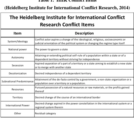
Conflict Items
Conflict items are material or immaterial goods pursued by
conflict actors via conflict measures (Heidelberg Institute for International Conflict Research, 2014).
Table 1: HIIK Conflict Items
(Heidelberg Institute for International Conflict Research, 2014)
Conflict Intensity Level
The six intensity levels presented by the institute have been aggregated into two levels; “Not violent conflicts” and “Violent conflicts” as shown in Table 2. HIIK includes in their analysis 260 countries, islands and territories; some countries have several
conflicts. A total of 414 conflicts are scored in 2013. For this study a country will get the highest score for any conflict in which it is engaged.
Item Description
System/Ideology Conflict actor aspires a change of the ideological, religious, socioeconomic or judicial orientation of the political system or changing the regime type itself National power The power to govern a state
Autonomy Attaining or extending political self-rule of a population within a state or of a dependent territory without striving for independence
Secession Aspired separation of a part of a territory or a state aiming to establish a new state or to merge with another state
Decolonization Desired independence of a dependent territory
Subnational PredominanceAttainment of the de-facto control by a government, a non-state organization or a population over a territory or a population. Resources Pursued possession of a natural resources or raw materials, or the profits gained thereof
Territory Desired change of the course of an international border
International Power Desired change aspired in the power constellation in the international system or a regional system therein
Other Residual category
The Heidelberg Institute for International Conflict
Research Conflict Items
Table 2: HIIK Intensity Level and Level of Violence
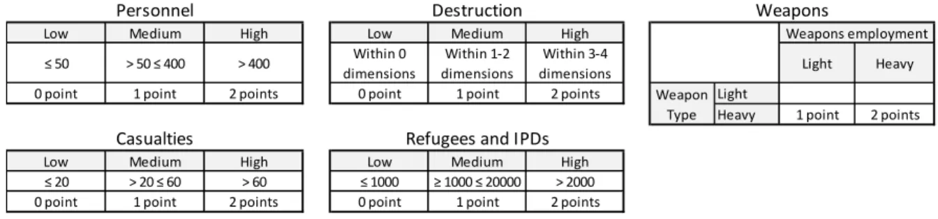
To assess the intensity levels of the violent conflicts HIIK measures five proxies; weapons, personnel, casualties, refugees and Internally Displaced Persons (IDPs) and destruction (Heidelberg Institute for International Conflict Research, 2014). These proxies are measured and scored for every region and every month. Table 3 shows the scoring method used by HIIK.
Table 3: HIIK Intensity Level Scoring Method
Method to select and screen independent variables and to impute missing data Twenty-two country statistic variables and four trend variables are considered in the initial analysis. Ten variables are considered from the CAA FACT study and three variables are considered from the CIA study. The study sponsor believed population migrations influenced violent conflict so refugee population seeking asylum and refugee
Intensity Level Terminology Level of Violence 0 No conflict 1 Dispute 2 Non-violent crisis 3 Violent crisis 4 Limited war 5 War Not violenct conflicts Violent conflicts
Low Medium High Low Medium High
≤ 50 > 50 ≤ 400 > 400 Within 0 dimensions
Within 1-2 dimensions
Within 3-4
dimensions Light Heavy
0 point 1 point 2 points 0 point 1 point 2 points Light
Heavy 1 point 2 points
Low Medium High Low Medium High
≤ 20 > 20 ≤ 60 > 60 ≤ 1000 ≥ 1000 ≤ 20000 > 2000
0 point 1 point 2 points 0 point 1 point 2 points
Weapons Personnel
Casualties
Destruction
Refugees and IPDs
Weapon Type
population of origin are both considered. Eight additional variables (Population density, population growth, rural population percent, arable land, birth rate, death rate and fertility rate) were deemed worthy of exploration by the study lead and are also considered in the study. Second order polynomials are introduced later. The four trend variables were included because of their potential to identify trends in a nation that could lead to violence. One additional variable, “Region”, is introduced later to explain the regional differences in the world; this variable proves key to the study.
Many of the 2013 data sets are not complete; this will require a two or three year lag in the model in order to predict 2015 nation states. Since this is 2014, predicting 2015 and beyond is the goal of this study. To predict 2015, the model will have to use 2012 and 2013 data. The 26 variables are listed in Table 4. Also listed in Table 4 are the year the dataset was first collected, the data lag and the number of nation entries for 2011-2013 for each variable. Fifteen of the country statistic data sets are from the World Bank; four are from the CIA world Fact book, one from Freedom House, one from the Center for Systemic Peace and one from and the Food and Agriculture organization of the United Nations. Eleven of the independent variables require a 2 year lag and use 2012 data to model 2015, 12 variables require a 3 year lag and 3 variables are locked and do not change. Yearly data is not available for “Regime Type”, “Ethnic Diversity” and “Religious Diversity” so these variables do not change from year to year and are considered locked.
Table 4: Country Statistic Variables
Most of the variables defined above have simple definitions but some of them require additional discussion. Following are expanded descriptions for these variables.
Trade (% of GDP) – This variable is the summation of two other World Bank statistics; Imports of goods and services (% of GDP) and Exports of goods and services (% of GDP)
Conflict in Bordering States – The CIA study cited Border Conflict as one of their significant variables. In this study, “border conflict” accounts for conflict in neighboring
2011 2012 2013 World Bank variables
1970 2 Population density (people per sq. km of land area) 181 181 180 1970 2 Population growth (annual %) 181 181 182 1970 2 Rural population (% of total population) 181 181 181 1970 3 Arable land (hectares per person) 181 181
1970 3 Birth rate, crude (per 1,000 people) 182 182 1970 3 Death rate, crude (per 1,000 people) 182 182 1970 3 Fertility rate, total (births per woman) 182 182 1990 3 Refugee population by country or territory of asylum (percent of pop) 160 159 1990 3 Refugee population by country or territory of origin (percent of pop) 180 280
1970 2 GDP/capita (current US$) 178 177 165 1970 3 Mortality rate, infant (per 1,000 live births) 182 182
1990 3 Improved water source (% of population with access) 174 172 1991 3 Unemployment, male (% of male labor force) (modeled ILO estimate) 171 171 1970 3 Life expectancy at birth, total (years) 182 182
1970 3 Trade (% of GDP) 167 146 92
CIA World Fact Book variables
2010 2 Conflict in Bordering States 182 182 182
Locked Regime type 182 182 182
Locked Ethnic diversity (Percent of dominant ethnic group) 180 180 180 Locked Religious diversity (Percent of dominant ethnic group) 178 178 178
Other
1973 2 Freedom (Average of Civil Liberties and Political Rights (scores 1 to 7)) 180 179 180 1946 2 Polity IV (Political behavior monitor (scores 1 to 10) 158 158 157 2001 3 Caloric Intake (Average caloric intake per person) 165 165
Trend Variables
2011 2 2 yr HIIK intensity level trend 182 182 182
1976 2 2 yr Freedom trend 180 180 180
1977 2 3 yr Freedom trend 180 180 180
1979 2 5 yr Freedom trend 180 180 180
Variables Number of entries per year Year of first
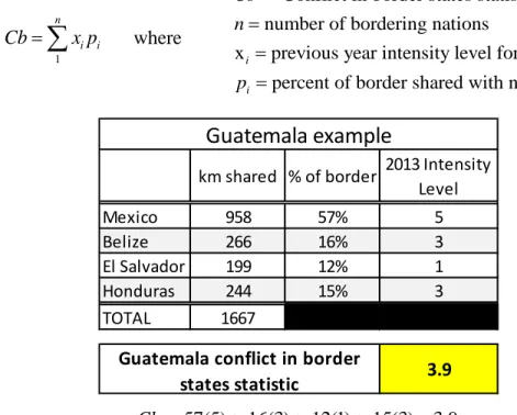
states and mimics a “bad neighbor” indicator. The CIA world Factbook publishes the shared land boundaries for each country. This variable will use the following formula to calculate a Border Conflict value for each nation. The formula and an example conflict score are shown in Table 5.
Table 5: Conflict in Bordering States Calculation
1
n i i
Cb=
∑
x p whereConflict in border states statistic number of bordering nations
x previous year intensity level for nation
percent of border shared with nation
i i Cb n i p i = = = = .57(5) .16(3) .12(1) .15(3) 3.9 Cb= + + + =
This variable will include a 2 year lag; a model for 2015 will include data from 2013. Twenty nine island nations that have no borders were imputed using JMP software.
Regime type – Regime type is cited by the CIA study as significant. The idea that different types of governments have different propensities for violent conflict necessitates
km shared % of border 2013 Intensity Level
Mexico 958 57% 5 Belize 266 16% 3 El Salvador 199 12% 1 Honduras 244 15% 3 TOTAL 1667
Guatemala example
Guatemala conflict in border
the need for this variable. The CIA World Factbook gives 57 different government descriptions for the 182 modeled nations. These 57 government types were initially mapped to 10 regime types. The variable “Regime type” was quickly removed from trial models because 10 nominative levels proved too many for a dataset that initially only included 114 nations. The old “Regime type” variable was partly responsible for overfitting the initial trial model. In order to include a “Regime type” variable in the model a “New Regime Type” variable was mapped from the original data, including only 3 types of regimes; “Central ruler/ ruling party”, “Democratic” and “Emerging,
transitional, recent change and disputed”. The old Regime variable and new Regime variable are shown in Table 6. For purposes of determing correlations and for factor analysis the regime types were mapped to numbers (Democratic = 1, Central ruler/ruling party = 2, Emerging, transitional, recent change, disputed = 3). In order to allow ordinal mapping of regime categories to a number the study assumes that democratic regimes are preferred to Central/ruling party regimes and both are preferred to Emerging, transitional, recent change, disputed regimes with regard to a nation being in a state of “Not in
conflict”. This assumption is supported by the corrleation between this mapped set and the dependent variable, shown later. The Freedom equation is shown in Equation 13.
Table 6: Regime Type
Civil liberties – Civil liberties is the allowance of freedom of expression and belief associational and organizational rights, rule of law, and personal autonomy without interference from the state. Civil Liberties is rated on a scale from 1 to 7; a score of “1” is best.
Political rights – Political rights is also rated on a scale from 1 to 7, it scores the ability of people to participate freely in the political process, including the right to vote, join political parties and elect representatives. A score of “1” is best.
Freedom – Civil Liberties and Political Rights are highly correlated. The Freedom statistic averages the two scores for the country, aggregating the correlated variables into one variable. This is the variable used in this study, not civil liberties or political rights. The FACT studies use both Political Rights and Civil Liberties as variables and the CIA study uses a variable name “State Discrimination”. The Freedom variable is introduced
New Class Total
Central ruler/ruling party 36
Democratic 137
Emerging, transitional, recent change, disputed 9
Grand Total 182
Reduced Regime Type Class Total Communist 4 Democracy 39 Dictatorship 2 Military Junta 1 Monarchy 24 Republic 107 Theocracy 2 Transitional Government 2 Disputed 1 Grand Total 182
variable proves to be one of the study’s most important variables. The equation for Freedom is shown in Equation 13.
Civil Liberty score + Political Rights score Freedom score =
2 Equation 13: Freedom Score
Polity IV – Polity IV Project records individual regime trends from 1946 to 2013. The Polity IV project is created by the Center for Systemic Peace (CSP) which is a not-for-profit organization that monitors political behavior in each of the world’s major states (Center for Systemic Peace, 2014). They record data for 167 Nation states. Each nation is scored between 0 and 10; 10 is the best. When a country is in a state of interruption, interregnum or transition the score was -66, -77 or -88. These scores were placeholders to identify nations that cannot be scored and cannot be used in the database. These data points were deleted, leaving only 157 nations for this variable. The missing data was later imputed using JMP software, discussed later.
Caloric intake – The Food and Agriculture Organization of the United Nations collects a myriad of food and agricultural data (United Nations, 2013). One of their metrics
measures the food supply of a country in Kilocalories per capita per day. This data is collected for years 2001 to 2011. 2011 data is used as a proxy for 2012 data to avoid using a 4 year lag throughout the model. All of the other variable datasets are complete through either 2012 or 2013 while Caloric intake only had data up to 2011.
Screening variables
Variable screening is used to remove some of the variables before initial model building. Multicollinearity, or near-linear dependence among the variables will cause problems in the model. High multicollinearity tends to produce unreasonably high logistic regression coefficients and can result in coefficients that are not statistically significant (Menard, 2001). Variance Inflation Factors (VIFs) are important
multicollinearity diagnostics (Menard, 2001). The equation for VIFs is shown in Equation 15.
Equation 15: VIF Calculation
VIFs larger than 10 imply serious problems with multicollinearity (Montomgery, 2012). According to Montgomery, VIFs that exceed 5 or 10 indicate that the associated
regression coefficients are poorly estimated. This study uses a VIF value of 10 as a threshold to remove variables. VIFs for all 26 initial variables are shown in the right column of Table 8. The values are calculated with JMP software using a database from 2011 to 2013. Five (boxed in red) variables have VIFs greater than 10.
Table 8: VIF Values for 26 Variables
Where:
is the coefficient of multiple
determination obtained from regressing on other regressor variables.
2 j R j x 2 1 1 j j VIF R = −
Table 9: VIF Values for 23 Variables
Removing the three variables reduces the correlations between the variables. Table 10 and Table 11 shows a heat map of the variable correlations before and after removing Birth Rate, Life Expectancy and Fertility Rate. There are substantially more high correlations in Table 10 than in Table 11. Regime type is a nominal data set and is not included in the tables. Although some high correlations still exist in the remaining variables, none of the VIF values are greater than 10. Some of the most correlated variables included the Freedom trend variables with each other, “Infant Mortality” with “Improved water” and “Freedom” with “Polity IV”. This is not surprising, as access to improved water decreases then infant mortality will naturally increase and the Freedom Score and Polity IV score are both scores of a nation’s political oppressiveness.
Model building set and Validation Set
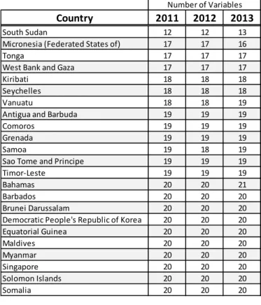
For the initial analysis, a model for 2011 and 2012 is developed and 2013 data is used to validate. Before the model can be built, the missing data needs to be imputed (filled in). For the 2011-2013 model and validation database only 345 out of 546 nations have data for all 23 variables. Unfortunately, often the nations with the worst data are the ones in the most danger of being in conflict. On average, a nation has 22.1 variables out of 23. The nation with the worst data is understandably South Sudan which is the world’s newest nation, gaining independence in 2006. This fledgling and tumultuous nation does not yet have the data infrastructure necessary for good data collection. Table 12 shows the nations with the worst data, ones that have complete data for 20 or fewer variables.
Table 12: Number of Variables per Nation; Nations with Worst Data
Country 2011 2012 2013
South Sudan 12 12 13
Micronesia (Federated States of) 17 17 16
Tonga 17 17 17
West Bank and Gaza 17 17 17
Kiribati 18 18 18
Seychelles 18 18 18
Vanuatu 18 18 19
Antigua and Barbuda 19 19 19
Comoros 19 19 19
Grenada 19 19 19
Samoa 19 18 19
Sao Tome and Principe 19 19 19
Timor-Leste 19 19 19
Bahamas 20 20 21
Barbados 20 20 20
Brunei Darussalam 20 20 20 Democratic People's Republic of Korea 20 20 20 Equatorial Guinea 20 20 20 Maldives 20 20 20 Myanmar 20 20 20 Singapore 20 20 20 Solomon Islands 20 20 20 Number of Variables
Data Imputation
The JMP software offers a method to impute data. Imputing analyzes similar values in other columns and rows to estimate the missing value (Hinrichs, 2010). JMP produces a new data table that duplicates the data table and replaces all missing values with estimated values (SAS Institute, 2015). Imputed values are expectations conditional on the non-missing values for each row. The mean and covariance matrix is used for the imputation calculation.
Methods to develop the Model
A method is needed to construct models now that the dependent and independent variables have been identified, screened and compiled into a model and validation dataset. Three method are introduced; two correlation methods and a least significant method. Models will be constructed using all methods and tested against each other using the Validation set prediction accuracy as the grading requirement.
Method 1: Correlation method
The correlation method will start with zero variables and add variables based upon significance. The variables with the highest correlation with the HIIK intensity levels will be tested first for inclusion in the model and no variables will be removed once they have been included. Table 13shows the variable correlations with the HIIK intensity level used for the testing order with this method. The correlation for regime type, which is nominal, is acquired by assigning values to the regime types (Democratic
This method will begin with all 23 variables and remove the least significant variable. The Effect Likelihood Ratio Test will be used to determine the least significant variable. One insignificant variable will be removed at a time and the model will be tested again to determine the next insignificant variable to remove. The prediction accuracy will be saved for each iteration in order to build the Signal to Noise Ratio chart described in chapter 4. The prediction accuracy is calculated using the formula in Figure 6.
Alternate Model: Only nations that enter into a violent conflict
Three methods were investigated to analyze only nations that are new to violent conflict. The first method uses a new database from 2009-2013, one that only includes nations that entered into violent conflict and their corresponding row of data from the previous year. The goal for this method is to build a model that predicts the year the nation transitions into violent conflict. The dependent variable remained the same as before except now the database was substantially smaller, only using nations new to conflict and their previous year. Twenty independent variables were considered. The three locked variables were omitted because they did not change between the years.
For the 2nd method a database was compiled of new nations to violent conflict in
addition to previous years when the nation was in a state of “Not violent conflict”. Similar to method 1, this method differs in that only nations with a period of “not in violent conflict” for at least 2 consecutive years before the transition to violence were included. The goal was to have a distinct period of “not violent conflict” years and then the “violent conflict” year. The alternate correlation method was used to construct a
The 3rd method involved analyzing the behavior of false positives and false
negatives in the four years following their false prediction. The premise is that the model believes they should be in conflict so they are likely candidates for conflict the next year or soon after. Nations falsely predicted will be analyzed the following years to determine the likelihood they will eventually transition to a violent conflict. This method will also look at different logistic probabilities. Recall the output of logistic regression is a probability that is rounded to either 0 or 1 using a threshold value with a default of .5. The higher the probability is, the more certain the model is that the nation will be in a violent conflict. A nation with a probability of .8 can be translated as the model is 80% certain the nation will be in a state of violent conflict for its predicted year. The study further analyzes nations at different probability levels. This method assumes the state of the nation remains constant over the future analyzed years.
Summary
Methodologies have been described for logistic regression, model building, sensitivity analysis and methods to predict nations new to violent conflict. The
dependent variable has been defined. The independent variables have been defined and screened. Two separate databases (2011-2013 & 2009-2013) have been constructed and missing data imputed. The next step uses these methods and data to construct models and conduct analysis.
IV. Analysis and Results
Chapter Overview
This chapter will use the methods described previously to construct trial models. These trial models will be assigned a name, such as Trial Model 1, and be compared to each other using the validation set prediction accuracy as the test for model goodness. The initial analysis is conducted using a database from 2011-2013. Two years are set aside to build the model (2011-2012) and one year is used to validate the model (2013). A few of the independent variables restrict the size of the database. After initial analysis these variables are removed from consideration and the database is allowed to expand. The second set of analysis uses a database from 2009-2013. Three years are set aside to build the model (2009-2011) and two years are used to validate the model (2012-2013). Factor Analysis and robustness of the confusion matrix cut off value are explored to gain insight on the problem.
Results of Constructing Logistic Regression Trial Models Method 1 - Correlation Method
The process described in chapter 3 is used for all the variables in the order listed in Table 13. Using this method, seven variables are accepted into the model at an alpha = .1 and six variables are accepted at an alpha = .05. The variable accepted at alpha = .1 and not at alpha = .05 is “2 yr Freedom trend”. A model of all the variables
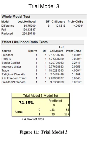
Polynomials are tested in the same order as main effects; see Table 13, using the same hypothesis tests. Polynomials can model a non-linear relationship between the dependent and independent variables. The results of this process are shown in Figure 11. Only Freedom*Freedom was added to the model. Water*Water was near the threshold, having a value of .1005 for Trial Model 3. A detailed description of one of the trial models is provided in a later section.
Figure 11: Trial Model 3
0 1
0 143 55 1 39 127 364 rows of data
Trial Model 3 Model Set
74.18% Predicted Actual
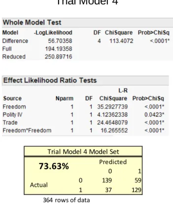
Method 2 – Alternate Correlation Method
Variables were tested in the same order as method 1 but variables were removed when their alpha value was greater than 0.1. 2nd order polynomials were also tested in the
same order. Trial Model 4 was constructed using this method and is shown in Figure 12.
Figure 12: Trial Model 4
Method 3 - Least Significant Variable Method
Method 3, starting with all of the variables and removing the least significant one until they are all significant at a certain threshold, is used to construct the next 5 models. The Signal to Noise Ratio Chart, shown in Figure 13, is calculated using the prediction accuracy for each iteration of removing a variable. These charts show the impact each
0 1
0 139 59
1 37 129
364 rows of data
Trial Model 4 Model Set
73.63% Predicted
Actual
Figure 14: Trial Models 5 & 6
All variables in Trial Model 5 and Trial Model 6 are raised to a 2nd order Polynomial and
tested in the same “least significant” method. Hierarchy is enforced, a main effect will not be removed if its 2nd order polynomial is insignificant and included in the model.
Three models are saved from this process, the results are shown in Figure 15 and the Signal to Noise Ratio Charts are shown in Figure 16 and Figure 17. Trial Model 7 includes all main effects and 2nd order polynomials from Trial Model 5 that are
significant at an alpha = .05, with the exception of one of the main effects. In this case GDP per capita has an Effects Likelihood Ratio Test value of .32 but its 2nd order
polynomial has a value of .018. Trial Model 8 includes all main effects and 2nd order
0 1
0 148 50
1 42 124
364 rows of data
Trial Model 5 Model Set 74.73% Predicted Actual 0 1 0 147 51 1 43 123 364 rows of data
Trial Model 6 Model Set 74.18% Predicted
Actual
Table 14: Trial Model Prediction Accuracy
Trial Model 7 has the best validation set prediction accuracy. This is also the only model whose prediction accuracy is greater in the validation set than in the model set, indicating a good fit. Trial Model 7 has 10 variables, including six main effects, one trend variable and three 2nd order polynomials. Statistical results for Trial Model 7 were
previously shown in Figure 15.
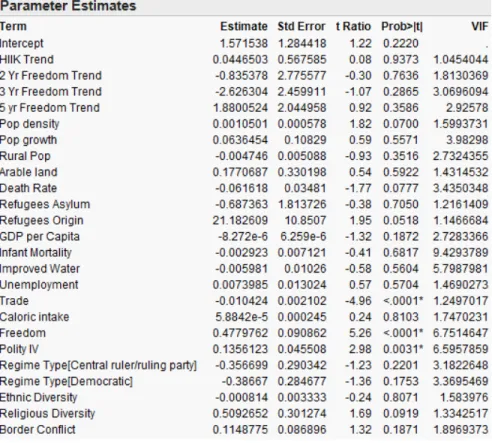
The coefficients for Trial Model 7 are shown in Table 15. The main effects are listed in order of significance, as determined by their effect likelihood ratio test statistic. It is important to note that the variable data was not normalized, which explains the large variety in the values of the coefficients.
Construction Method Model #Trial VariablesNum of Model Set Validation Set
Model and Validation Set 1 7 73.1% 72.0% 72.7% 2 6 74.2% 71.4% 73.3% 3 8 74.2% 74.2% 74.2% Method 2 - Alternate 4 4 73.6% 73.1% 73.4% 5 8 74.7% 74.7% 74.7% 6 5 74.2% 72.0% 73.4% 7 10 75.3% 76.4% 75.6% 8 7 76.1% 72.5% 74.9% 9 7 73.4% 73.1% 74.9% Prediction Accuracy Method 1 - Correlation Method Method 3 - Least Significant Method