MULTIVARIATE DATA MODELING
AND ITS APPLICATIONS TO
CONDITIONAL OUTLIER DETECTION
by
Charmgil Hong
B.S.E., Handong Global University, 2010
Submitted to the Graduate Faculty of
the Dietrich School of Arts and Sciences in partial fulfillment
of the requirements for the degree of
Doctor of Philosophy
University of Pittsburgh
2017
UNIVERSITY OF PITTSBURGH
THE DIETRICH SCHOOL OF ARTS AND SCIENCES
This dissertation was presented by
Charmgil Hong
It was defended on August 9, 2017 and approved by
Milos Hauskrecht, PhD, Professor, Department of Computer Science
Rebecca Hwa, PhD, Associate Professor, Department of Computer Science
Adriana Kovashka,PhD, Assistant Professor, Department of Computer Science
Gregory Cooper, MD, PhD, Professor, Department of Biomedical Informatics
Dissertation Director: Milos Hauskrecht,PhD, Professor, Department of Computer Science
Copyright c byCharmgil Hong
MULTIVARIATE DATA MODELING AND ITS APPLICATIONS TO CONDITIONAL OUTLIER DETECTION
Charmgil Hong, PhD
University of Pittsburgh, 2017
With recent advances in data technology, large amounts of data of various kinds and from various sources are being generated and collected every second. The increase in the amounts of collected data is often accompanied by increase in the complexity of data types and objects we are able to store. The next challenge is the development of machine learning methods for their analyses. This thesis contributes to the effort by focusing on the analysis of one such data type, complex input-output data objects with high-dimensional multivariate binary output spaces, and two data-analytic problems: Multi-Label Classification and Conditional Outlier Detection.
First, we study the Multi-label Classification (MLC) problem that concerns classification of data instances into multiple binary output (class or response) variables that reflect differ-ent views, functions, or compondiffer-ents describing the data. We presdiffer-ent three MLC frameworks that effectively learn and predict the best output configuration for complex input-output data objects. Our experimental evaluation on a range of datasets shows that our solutions outperform several state-of-the-art MLC methods and produce more reliable posterior prob-ability estimates.
Second, we investigate theConditional Outlier Detection(COD) problem, where our goal is to identify unusual patterns observed in the multi-dimensional binary output space given their input context. We made two important contributions to the definition and solutions of COD. First, by observing a gap in between the development of unconditional and
con-ditional outlier detection approaches, we propose a ratio of outlier scores (ROS) that uses a pair of unconditional scores to calculate the conditional scores. Second, we show that by applying the chain decomposition of the probabilistic model, the probabilistic multivariate COD score decomposes to a set of probabilistic univariate COD scores. This decomposition can be subsequently generalized and extended to a broad spectrum of multivariate COD scores, including the new ROS score and its variants, leading to a new multivariate condi-tional outlier scoring framework. Through experiments on synthetic and real-world datasets with simulated outliers, we provide empirical results that support the validity of our COD methods.
TABLE OF CONTENTS
PREFACE . . . xvii
1.0 INTRODUCTION . . . 1
1.1 MULTI-LABEL CLASSIFICATION . . . 3
1.2 CONDITIONAL OUTLIER DETECTION . . . 6
1.3 OUR CONTRIBUTIONS . . . 9
1.4 ORGANIZATION OF THE THESIS . . . 10
2.0 BACKGROUND . . . 11
2.1 MODELING AND PREDICTION OF MULTIVARIATE RESPONSES. . . 11
2.1.1 Binary Relevance – Why Learning Independent Classification Models is Not Enough . . . 12
2.1.2 Early Multi-label Classification Approaches . . . 13
2.1.3 Output Coding Approaches . . . 14
2.1.4 Classifier Chains and Its Extensions . . . 14
2.1.5 Multi-Label Conditional Random Fields . . . 15
2.1.6 Multi-Dimensional Bayesian Network Classifiers . . . 16
2.1.7 Ensemble Approaches . . . 17
2.1.8 Our Work . . . 18
2.2 CONDITIONAL OUTLIER DETECTION . . . 19
2.2.1 Unconditional Outlier Detection Approaches . . . 20
2.2.1.1 Distance-based Approaches . . . 20
2.2.1.2 Density-based Approaches . . . 21
2.2.1.4 Deviation-based Approaches . . . 24
2.2.1.5 Classification-based Approaches . . . 25
2.2.1.6 Approaches for High-dimensional Data . . . 27
2.2.2 Conditional Outlier Detection . . . 28
2.2.2.1 Multivariate Conditional Outlier Detection . . . 29
2.2.3 Our Work . . . 29
3.0 MODELING AND PREDICTION OF MULTIVARIATE RESPONSES 31 3.1 PROBLEM DEFINITION AND NOTATION . . . 32
3.2 CONDITIONAL TREE-STRUCTURED BAYESIAN NETWORKS. . . 33
3.2.1 Representation . . . 34
3.2.2 Learning the Structure . . . 35
3.2.2.1 Complexity . . . 37
3.2.3 Prediction . . . 38
3.2.3.1 Complexity . . . 39
3.2.4 Experiments . . . 39
3.2.5 Discussion . . . 39
3.3 MIXTURES-OF-CONDITIONAL TREE-STRUCTURED BAYESIAN NET-WORKS . . . 40
3.3.1 Preliminary: Mixtures-of-Trees Framework . . . 40
3.3.2 Representation . . . 42 3.3.3 Parameter Learning . . . 43 3.3.3.1 Complexity . . . 45 3.3.4 Structure Learning . . . 46 3.3.4.1 Complexity . . . 48 3.3.5 Prediction . . . 48 3.3.6 Experiments . . . 49 3.3.6.1 Datasets . . . 49 3.3.6.2 Methods . . . 49 3.3.6.3 Evaluation Metrics . . . 50 3.3.6.4 Results. . . 51
3.3.7 Discussion . . . 55
3.4 MULTI-LABEL MIXTURES-OF-EXPERTS . . . 55
3.4.1 Preliminary: Mixtures-of-Experts Framework . . . 56
3.4.2 Representation . . . 59 3.4.3 Parameter Learning . . . 61 3.4.3.1 Complexity . . . 63 3.4.4 Structure Learning . . . 64 3.4.4.1 Complexity . . . 66 3.4.5 Prediction . . . 66 3.4.6 Experiments . . . 67 3.4.6.1 Datasets . . . 67 3.4.6.2 Methods . . . 67 3.4.6.3 Evaluation Metrics . . . 68 3.4.6.4 Results. . . 68 3.4.7 Discussion . . . 70 3.5 SUMMARY . . . 71
4.0 CONDITIONAL OUTLIER DETECTION. . . 73
4.1 PROBLEM DEFINITION AND NOTATION . . . 75
4.2 UNIVARIATE CONDITIONAL OUTLIER DETECTION . . . 76
4.2.1 Probabilistic Approach to Univariate Conditional Outlier Detection . 76 4.2.1.1 Data Modeling . . . 76
4.2.1.2 Outlier Scoring . . . 78
4.2.1.3 Limitations of Probabilistic Models . . . 79
4.2.2 Univariate Conditional Outlier Detection with Unconditional Outlier Detection Methods . . . 80
4.2.2.1 Ratio of Outlier Scores . . . 80
4.2.2.2 Local Outlier Factor . . . 82
4.2.2.3 Ratio of Outlier Scores on Discriminative Projections . . . 82
4.2.3 Experiments . . . 85
4.3 MULTIVARIATE CONDITIONAL OUTLIER DETECTION . . . 94
4.3.1 Probabilistic Approach to Multivariate Conditional Outlier Detection 94 4.3.1.1 Data Modeling . . . 96
4.3.1.2 Outlier Scoring . . . 96
4.3.1.3 Decomposable Data Model with Circular Dependences . . . . 98
4.3.1.4 Outlier Scoring with Reliability Weights . . . 99
4.3.1.5 Experiments . . . 101
4.3.2 Multivariate Conditional Outlier Detection with Ratio-based Outlier Scoring . . . 110
4.3.2.1 Ratio of Outlier Scores on Multi-dimensional Discriminative Projections . . . 112
4.3.2.2 Alternative Multivariate Conditional Outlier Scoring Approaches113 4.3.2.3 Experiments . . . 114
4.3.3 Discussion . . . 126
4.4 SUMMARY . . . 128
5.0 CONCLUSIONS . . . 140
5.1 MODELING AND PREDICTION OF MULTIVARIATE RESPONSES. . . 140
5.1.1 Contributions . . . 140
5.1.2 Open Questions . . . 141
5.2 CONDITIONAL OUTLIER DETECTION . . . 142
5.2.1 Contributions . . . 143
5.2.2 Open Issues . . . 143
LIST OF TABLES
2.1 The joint distribution of class variables Y1 and Y2 conditioned on instance x.
The optimal (MAP) prediction is h∗(x) = (Y1 = 1, Y2 = 0). . . 13
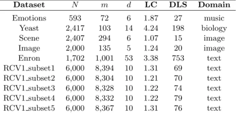
3.1 Datasets characteristics (N: number of instances, m: number of features, d: number of classes, LC: label cardinality, DLS: distinct label set, DM: domain). 49
3.2 Performance of each method on the benchmark datasets in terms of exact match accuracy (EMA; higher value is better). Marker∗/~indicates whether MC is statistically superior/inferior to the compared method (using paired t-test at 0.05 significance level). The last row shows the total number of win/tie/loss for MC against the compared method (e.g., #win is how many times MC significantly outperforms that method). . . 52
3.3 Performance of each method in terms of conditional log-likelihood loss (CLL-loss; smaller value is better). Marker∗/~indicates whether MC is statistically superior/inferior to the compared method (using paired t-test at 0.05 signif-icance level). The last row shows the total number of win/tie/loss for MC against the compared method. . . 52
3.4 Performance of each method in terms of micro F1 (higher value is better). Marker∗/~indicates whether MC is statistically superior/inferior to the com-pared method (using paired t-test at 0.05 significance level). The last row shows the total number of win/tie/loss for MC against the compared method. 53
3.5 Performance of each method in terms of macro F1 (higher value is better). Marker∗/~indicates whether MC is statistically superior/inferior to the com-pared method (using paired t-test at 0.05 significance level). The last row shows the total number of win/tie/loss for MC against the compared method. 53
3.6 Datasets characteristics (N: number of instances, m: number of features, d: number of classes, LC: label cardinality, DLS: distinct label set, DM: domain). 67
3.7 Performance of each method on the benchmark datasets in terms of exact match accuracy (EMA; higher value is better). Numbers in parentheses show the relative ranking of the method on each dataset. The best methods (by paired t-test at α= 0.05) are shown in bold. The last row shows the average ranking of the methods. . . 69
3.8 Performance of each method on the benchmark datasets in terms of conditional log-likelihood loss (CLL-loss; smaller value is better). Numbers in parentheses show the relative ranking of the method on each dataset. The best methods (by paired t-test at α = 0.05) are shown in bold. The last row shows the average ranking of the methods. . . 69
4.1 Average precision-alert rate in alert rate = [0.00,0.01] range (APAR[0.00,0.01]) and area under the precision-recall curve (AUPRC) for the conditional outlier detection on synthetic datasetsSD1 andSD2. Numbers shown in bold indicate the best results on each experiment set (by paired t-test at α= 0.05). Higher APAR/AUPRC is better. . . 88
4.2 Average precision-alert rate in alert rate = [0.00,0.01] range (APAR[0.00,0.01]) and area under the precision-recall curve (AUPRC) for the conditional outlier detection on synthetic datasetsSD3 andSD4. Numbers shown in bold indicate the best results on each experiment set (by paired t-test at α= 0.05). Higher APAR/AUPRC is better. . . 89
4.3 Average precision-alert rate in alert rate = [0.00,0.01] range (APAR[0.00,0.01]). Numbers shown in bold indicate the best results on each experiment set (by paired t-test at α= 0.05). Higher APAR is better. . . 92
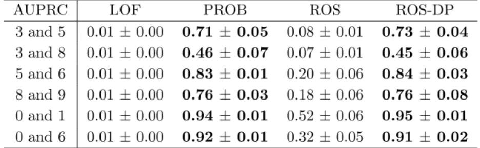
4.4 Area under the precision-recall curve (AUPRC). Numbers shown in bold in-dicate the best results on each experiment set (by paired t-test at α= 0.05). Higher AUPRC is better. . . 92
4.5 Dataset characteristics (N: number of instances, m: input dimensionality, d: output dimensionality). . . 102
4.6 Average precision-alert rate in [0.00, 0.01] (APAR[0.00,0.01]). Numbers shown
in bold indicate the best results on each experiment set (by paired t-test at
α= 0.05). Dashes (-) indicate the sets that we cannot create due to low output dimensionality. . . 107
4.7 Area under the precision-recall curve. Numbers shown in bold indicate the best results on each experiment set (by paired t-test at α= 0.05). Dashes (-) indicate the sets that we cannot create due to low output dimensionality. . . 108
4.8 Parameters for the data generation of SD5 and SD6.. . . 117
4.9 Average precision-alert rate in [0.00, 0.01] (APAR[0.00,0.01]). Numbers shown
in bold indicate the best results on each experiment set (by paired t-test at
α= 0.05). . . 120
4.10 Area under the precision-recall curve. Numbers shown in bold indicate the best results on each experiment set (by paired t-test at α= 0.05). . . 121
4.11 Dataset characteristics (N: number of instances, m: input dimensionality, d: output dimensionality). . . 122
4.12 Average precision-alert rate in [0.00, 0.01] (APAR[0.00,0.01]). Numbers shown in bold indicate the best results on each experiment set (by paired t-test at
α= 0.05). Dashes (-) indicate the sets that we cannot create due to low output dimensionality. . . 123
4.13 Area under the precision-recall curve. Numbers shown in bold indicate the best results on each experiment set (by paired t-test at α= 0.05). Dashes (-) indicate the sets that we cannot create due to low output dimensionality. . . 124
LIST OF FIGURES
1.1 Data objects with multiple output variables. . . 2
2.1 An example MBC [van der Gaag and de Waal, 2006, Bielza et al., 2011] which defines the joint probability distribution over three class variables {Y1, Y2, Y3} and four feature variables {X1, X2, X3, X4}. . . 16
2.2 Example where the use of local density is desired. . . 21
2.3 Difference between the neighborhoods used by LOF and COF (when k= 6). 22 2.4 An example multi-granularity problem. . . 23
2.5 Depth-based outlier detection. . . 24
2.6 Classification-based outlier detection. . . 25
3.1 An example CTBN. . . 34
3.2 The complete directed graph G for four class variables. The weights of the edges are defined using Equations (3.5) and (3.6). The optimal CTBN is obtained by running a maximum branching algorithm on G. . . 36
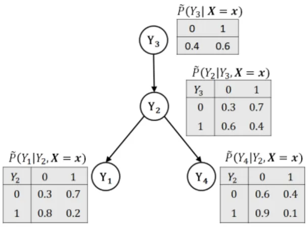
3.3 An example showing the CPTs of a CTBN model for a specific instance x. . 39
3.4 An example MC. . . 42
3.5 Example models in the classifier chains family. . . 57
3.6 An example of ML-ME. . . 60
4.1 Probabilistic conditional outlier detection.. . . 77
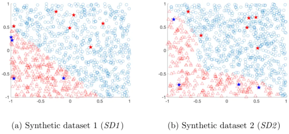
4.2 Two synthetic datasets (SD1 and SD2) with example conditional outliers (marked with a star). Colors represent the output assignment (red= 1;blue= 0). 87 4.3 MNIST dataset [LeCun et al., 1998]. . . 90
4.4 Precision-alert rates (PAR) at alert rates (detection thresholds) between 0.00 and 0.04. The vertical dashed lines at alert rate = 0.01 indicate where the alert rate coincides with the simulated outlier ratio. . . 91
4.5 Precision-alert rate (PAR) at alert rates (detection thresholds) between 0.00 and 0.04. The vertical dashed lines at alert rate = 0.01 indicate where the alert rate coincides with the simulated outlier ratio. . . 104
4.6 Precision-alert rate (PAR) at alert rates (detection thresholds) between 0.00 and 0.04. The vertical dashed lines at alert rate = 0.01 indicate where the alert rate coincides with the simulated outlier ratio. . . 105
4.7 Precision-alert rate at alert rates (detection thresholds) between 0.00 and 0.04. The vertical dashed lines at alert rate = 0.01 indicate where the alert rate coincides with the simulated outlier ratio. . . 106
4.8 Synthetic datasets 5, 6 (SD5 andSD6; the first row) and example conditional outliers (marked with a star; the second row). . . 116
4.9 Precision-alert rate (PAR) on SD5. Each plot draws PAR at alert rates (de-tection thresholds) between 0.00 and 0.04. The vertical dashed lines at alert rate = 0.01 indicate where the alert rate coincides with the simulated outlier ratio. . . 118
4.10 Precision-alert rate (PAR) on SD6. Each plot draws PAR at alert rates (de-tection thresholds) between 0.00 and 0.04. The vertical dashed lines at alert rate = 0.01 indicate where the alert rate coincides with the simulated outlier ratio. . . 119
4.11 Precision-alert rate (PAR) on Mediamill (outlier dimensionality = {5.0, 10.0, 20.0, 50.0}%). . . 130
4.12 Precision-alert rate (PAR) on Yahoo-business (outlier dimensionality = {5.0, 10.0, 20.0, 50.0}%). . . 131
4.13 Precision-alert rate (PAR) on Yahoo-arts (outlier dimensionality = {5.0, 10.0, 20.0, 50.0}%). . . 132
4.14 Precision-alert rate (PAR) on Bibtex (outlier dimensionality ={5.0, 10.0, 20.0, 50.0}%). . . 133
4.15 Precision-alert rate (PAR) on Enron (outlier dimensionality ={5.0, 10.0, 20.0, 50.0}%). . . 134
4.16 Precision-alert rate (PAR) on Birds (outlier dimensionality = {5.0, 10.0, 20.0, 50.0}%). . . 135
4.17 Precision-alert rate (PAR) on Cal500 (outlier dimensionality ={5.0, 10.0, 20.0, 50.0}%). . . 136
4.18 Precision-alert rate (PAR) on Yeast (outlier dimensionality = {10.0, 20.0, 50.0}%). . . 137
4.19 Precision-alert rate (PAR) on Rcv1sub1-top10 (outlier dimensionality ={10.0, 20.0, 50.0}%). . . 138
4.20 Precision-alert rate (PAR) on Rcv1sub3-top10 (outlier dimensionality ={10.0, 20.0, 50.0}%). . . 139
LIST OF ALGORITHMS 1 Find-an-optimal-CTBN-structure . . . 37 2 Predict-CTBN. . . 38 3 Learn-MC-parameters . . . 45 4 Learn-ML-ME-parameters . . . 63 5 Find-an-optimal-chain-structure . . . 65
PREFACE
The work presented in this thesis would not have been possible without the help and support of many people. I take this opportunity to extend my sincere gratitude and appreciation to all those who made this thesis possible.
I would like to express my heartfelt gratitude to my advisor, Milos Hauskrecht, who has guided me throughout my Ph.D. journey. Milos introduced me to this exciting field of machine learning and data mining and trained me to his own high standards. Through the lectures, seminars, projects, and discussions, he has molded me into the independent researcher I am today. All along, Milos has been someone who always trusted and supported me in literally every situation.
I am very grateful to our former post-doc, Iyad Batal, who was an inspiring mentor, as well as a good friend of mine. Iyad got me interested in multi-label classification. Many parts of the thesis have been done in collaboration with him. I also would like to thank Sangyuen Cho, who first exposed me to the academic research experience when I was a visiting undergraduate student here at Pitt and offered me a lot of help when I joined back as a graduate student.
I would like to thank my thesis committee members, Rebecca Hwa, Adriana Kovashka, and Greg Cooper, for their valuable feedback and insightful discussions during my thesis defense. Greg was also a member of our research team investigating various clinical/medical projects. It was a privilege to work with him and also with Gilles Clermont and Shyam Visweswaran on these important projects. I am grateful for their positive influence on me that promoted and developed my scientific thinking and reasoning skills.
Besides Iyad, I was also fortunate to work with extraordinary lab mates, Quang Nguyen, Salim Malakouti, Zhipeng Patrick Luo, and Siqi Liu, on our awesome projects on clinical
outlier monitoring and alerting. I would like to thank all of them for the collaborations and our endless discussions. I also want to thank other lab alumni: Hamed Valizadegan, Lei Wu, Michal Valko, Dave Krebs, Saeed Amizadeh, Eric Heim, and Zitao Liu.
During my Ph.D. career, I spent two amazing summers at Bosch RTC and Siemens CT. I would like thank to my mentors and managers, Rumi Ghosh, Soundar Srinivasan, Dmitriy Fradkin, and Amit Chakraborty, who motivated and helped me to stretch my boundaries and grow in my abilities. I also want to extend my thanks to Zubin Abraham, Heng Wang, Mahmudur Rahman, Congrui Yi, Goktug Cinar, Ruobing Chen, Mohammad Shokoohi-Yekta, Ioannis Akrotirianakis, Ramamani Ramaraj, Sindhu Suresh, Chao Yuan, Bernardo Hermont, Xiaoyan Xiang, Tugba Kulahcioglu, Chabin Guillaume, Xi He, Jie Liu, Inbeom Song, Wonki Yoon and his family, Hyun-a Song and Youngjin Kim, Pastor Jungwook Kang and Korean Church of Love, Pastor Dongwook Kim and Princeton Korean Presbyterian Church, who made my stay just like a home away from home.
I am grateful to our tech staff, Bob Hoffman, Terry Wood, the late Russ Howard, Adam Hobaugh, and Walter Gibson, who were always on standby for trouble calls and made sure the Elements cluster is running 24/7. I would also like to thank our administrative staff, including Keena Walker, Karen Dicks, Michele Thomas, Deb Lauro, the late Kathleen Allport, Wendy Bergstein, and Nancy Kreuzer, whose support is vital to our department.
My life in Pittsburgh would have been merely monotone and even gloomy if not for these people: Jinyoung Jung and Seunghyun Yoon, Jieun Kim, Chilman Bae and Eunjoo Kim, Nohyun Park and his family, Eun-kyung Hong and Chanil Jung, Seungjae Baek and his family, Heekwon Park and his family, Kiyeon Lee, Ju-young Jung, Hyungbo Shim and Ji Young Song, Okrae Kim and his family, Daesup Lee and his family, Hyunjin Abraham Lee, Rakan Maddah, Phillip Walker, Shih-Yi James Chien, Donghun Don Lee, Judong Lee, Donghyun Ku and Gahgene Gweon, Pastor Hongkil Lee and his family, Pastor Youngsun Cho and Pittsburgh Korean Assembly of God, Pastor Jonathan Kim and State College Korean Church, Pastor Paul Becker and First Presbyterian Church of Bakerstown. I would like to mention and express my appreciation to the faculty members of Handong Global University and many friends I met there, especially the members ofSLE – I know many of you still keep me in your prayers. I also want to mention and thank Jinhun Isaac Park, who generously
helped me proofread this thesis.
Lastly, my biggest love and appreciation go to my wonderful family. I am deeply thankful to my closest friend and wife, Hyun Joo, and our proud daughter, Cielle, who both have been absolute blessings to me. I thank my parents and parents-in-law, who have made innumerable sacrifices throughout their life to bring me and Hyun Joo up. I would like to send my love to my extended families in New Jersey and everywhere in Korea for their sincere love and prayers.
1.0 INTRODUCTION
With recent advances in data acquisition and storage technologies, vast amounts of data of various kinds and from various sources are being generated and collected every second. The increase in the amounts of collected data is often accompanied by the increase in the complexity of data types and objects we are able to store: univariate time series data are being replaced with multivariate time series, low-dimensional data objects are becoming high-dimensional, input-output data pairs for classification tasks include multiple (not just one) class labels, etc. All these prompt the development of new data analytic and machine learning solutions that are scalable to these new types of data and capable of overcoming the new complexity challenges.
This thesis focuses on the development of analytic methods for one such data type: complex input-output data objects with high-dimensional multivariate binary output spaces. The input-output data objects are typically used for classification and annotation purposes and a large number of data analytic and modeling algorithms have been developed over many years to solve them. However, the majority of them assume that data instances are linked to simple (univariate) class variable. Much less research and solutions are available when data objects are associated with multiple class variables. Examples of real-world problems when data objects come with multiple class variables are:
• Document topic classification: In text classification, a document can cover multiple
predefined topics [Kazawa et al., 2005, Zhang and Zhou, 2006]. For example, a news ar-ticle may belong topolitics andeconomics. As in the image/video classification example, these topics can be represented by a set (vector) of mutually non-exclusive indicators.
Figure 1.1: Data objects with multiple output variables.
image (or video) can be annotated with multiple tags [Boutell et al., 2004, Qi et al., 2007a]. For example, an image can be tagged with bird, cloud, and sky. Typically, such annotations are defined by an indicator vector, where each element represents a keyword.
• Music emotion recognition: In detecting emotions from music, each time-varying
music feature sequence is labeled with combinations of different emotions such as happy, sad, angry, calm, and so on [Trohidis et al., 2011, Kim et al., 2010]. Given a predefined set of emotions, the labels can be coded as a binary vector where each element represents an emotion class.
• Gene functional annotation: In gene functional analysis, a single gene may be
as-sociated with several functionalities, which can be represented as a vector of functional class variables [Clare and King, 2001, Zhang and Zhou, 2006].
• Medication prescriptions in electronic health records (EHR): In hospitals, a
patient may receive multiple medications in a prescription. Such records of medication orders can be expressed in a vector where the elements denote whether individual medi-cations are ordered or not [Hauskrecht et al., 2007, Hauskrecht et al., 2010, Hauskrecht
et al., 2013, Hauskrecht et al., 2016].
The main goal of the thesis is to develop computational methods that find data ob-jects with abnormal (unusual) input and output associations in the above described data collections. There are two fundamental questions that arise in addressing this goal:
Question 1 - Representation or definition of normality: For given input-output data
objects, how should one obtain the representation or definition of normal (usual) data?
Question 2 - Measures of abnormality: Given a representation/definition of normal
data, how should one measure and identify the abnormality of individual data object? To answer the questions, we hypothesize that we can adopt machine learning approaches to build statistical models representing the input-output patterns of the population and, in turn, that we can utilize the resulting representation to analyze data objects for abnormalities by assessing normalcy or deviation from expected patterns. Accordingly, our data analytic and algorithm development work in this thesis will focus on the following two problems that are defined on data with multivariate binary output:
1. Multi-Label Classification which is pertinent to the question of how to learn and
predict the best output (response) from complex input-output data. We study existing solutions to the multi-label classification problem and investigate ways to acquire more accurate and efficient data representations.
2. Conditional Outlier Detection which is concerned with how toidentify unusual
out-put patterns in multivariate conditional data. To our knowledge, no precedent work has focused on this specific research problem. We conduct an exploratory study to formalize a definition of conditional outlier detection and propose effective solutions to the problem. Below we briefly introduce the two problems and our solutions.
1.1 MULTI-LABEL CLASSIFICATION
In the traditional supervised learning scenarios, each data instance (represented by an input vector) is assumed to be associated with a single class label (output). Accordingly, the
process of learning from data to predict class labels can be described as seeking unidirectional dependence relations from input to output. When it comes to data with high-dimensional multivariate output, however, the same approach may not properly address the task because of the following properties of the data: (1) each output variable is not only dependent on input, but also dependent on other output variables – e.g., in the semantic image analysis example above, knowing that an image is tagged withbird may increase the possibility of the image being tagged withsky – and (2) the number of all possible output combinations grows exponentially to the output dimensionality – e.g., in the document classification example, if the number of all topics is d, the number of all possible topic combinations is 2d. These properties apparently make the classification task larger and harder. More specifically, to learn a classifier, one has to capture the dependences in both input-output and output-output relations. To predict the best output-output, one has to evaluate exponentially many label configurations. Consequently, to effectively perform classification on data with multivariate output, more sophisticated yet efficient supervised learning methods are required.
The problem of classification on data with multiple binary class variables, which reflect different views, functions, or components describing the data, is often referred to in the literature as Multi-label Classfication (MLC) [Tsoumakas et al., 2010, Zhang and Zhou, 2013]. The goal of MLC is to learn a function from data that assigns to each data instance, represented by a continuous feature vector (input), a binary vector of class labels (output). Early MLC methods [Clare and King, 2001, Boutell et al., 2004] assumed that all class variables are conditionally independent of each other, and learned individual classification functions to predict each output dimension separately. Obviously, this does not suffice to address the MLC problem, because the methods ignore all dependences among different class variables. Realizing the deficiency of the early solutions, a number of approaches have been developed and proposed to better model the relations among class variables. These include the methods using two levels of classifiers [Godbole and Sarawagi, 2004, Cheng and H¨ullermeier, 2009], multi-label extension of the k-nearest neighbor algorithm [Zhang and Zhou, 2007], error-correcting output coding approach [Hsu et al., 2009, Zhang and Schneider, 2012], classifier chains methods [Read et al., 2009, Dembczynski et al., 2010], multi-dimensional Bayesian networks [van der Gaag and de Waal, 2006,Bielza et al., 2011],
etc. However, each of the solutions has its own limits in terms of either optimality or complexity and scalability.
In this thesis, we present three MLC frameworks that effectively learn and predict the best output from complex input-output data objects. In the first solution, we assume that dependences among class variables are restricted and follow adirected treestructure. The tree structure can represent limited dependence relations in the output space, where each output variable can be conditioned (dependent) on at most one other output variable (its parent in the tree). The benefit is that this restriction lets us define efficient learning and prediction methods. We develop a learning algorithm that efficiently discovers the optimal tree structure from a pairwise conditional dependence analysis, and a linear-time prediction algorithm that finds the best class labels for a given input. We implement the ideas using a special Bayesian network, whose conditional distributions are defined using a set of probabilistic classifier functions. We refer to the model asConditional Tree-structured Bayesian Networks (CTBN; Section3.2).
Though the tree-structure assumption facilitates efficient learning and prediction in the CTBN framework, yet it may restrict a full recovery of the underlying dependence relations especially when the true dependences do not follow a tree. To alleviate this, we propose and build a mixture ensemble framework for MLC that leverages the computational advantages of CTBN and the abilities of mixtures that compensate for the tree-structure restrictions. In particular, we extend the Mixtures-of-Trees [Meil˘a and Jordan, 2000] framework, which is originally a generative framework that models multi-dimensional discrete data, to incorporate multiple CTBNs as its base models. Consequently, our mixture can learn various dependence relations, which a single tree-structured model cannot capture, and combine them to make ensemble predictions that achieve a higher predictive accuracy. Our second MLC solution is referred to as Mixtures-of-Conditional Tree-structured Bayesian Networks (Section 3.3).
Lastly, we further refine the above mixture solution by allowing the base MLC models to have different structural assumptions other than a tree (e.g., chain [Read et al., 2009]). Using the Mixtures-of-Experts [Jacobs et al., 1991] framework, our approach captures different input–output and output–output relations that tend to change across data. As a result, we can recover a rich set of dependence relations that a single MLC model cannot capture due to
its modeling simplifications. We refer to this last solution asMulti-Label Mixtures-of-Experts (Section 3.4).
Note that our MLC solutions presented in this thesis are based on the structured proba-bilistic graphical models [Koller and Friedman, 2009,Bakir et al., 2007,Nowozin et al., 2014], which provide the principles and techniques that support probabilistic model construction, learning, and inference for complex data. Accordingly, at the end of the learning process, our methods produce a well-defined model of posterior class probabilities that is extremely useful not only for prediction, but also for decision making [Raiffa, 1997, Berger, 1985] and for performing any inference over subsets of output class variables. In contrast to this, the majority of existing MLC methods aim to only identify the best output configuration for the given input.
The conditional outlier detection problem, which we will introduce next, is one of such problems that can be effectively solved by utilizing our MLC models and methods. While there are other types of problems that would benefit from our solutions, as we will describe shortly, conditional outlier detection in multi-dimensional output spaces is particularly less studied in the literature despite its potential importance. In the second half of the thesis, we conduct an investigation on how to effectively approach and solve this specific type of outlier detection problem.
1.2 CONDITIONAL OUTLIER DETECTION
Outlier detection [Markou and Singh, 2003, Kriegel et al., 2010, Aggarwal, 2017, Pimentel et al., 2014] is a data analysis method that aims to find atypical behaviors, unusual out-comes, or erroneous readings and annotations in data.1 It has been an active research topic
in data mining and machine learning communities and frequently used in various appli-cations to identify rare and interesting data patterns that may be associated with either beneficial or malicious events such as fraud identification [Fawcett and Provost, 1997,Wang, 2010], network intrusion surveillance [Tan et al., 2002, Garcia-Teodoro et al., 2009], disease
outbreak detection [Wong et al., 2003], patient monitoring for preventable adverse events (PAE) [Hauskrecht et al., 2007,Hauskrecht et al., 2013],etc. It is also utilized as a primary data preprocessing step that helps to remove noisy or irrelevant signals in data [Hodge and Austin, 2004, Liu et al., 2004].
Despite huge effort and progress in outlier detection research, however, the majority of existing methods are designed only to detect unconditional outliers, that are unusual data instances manifested in the joint space of all data attributes. Such methods may not work when one wants to identify conditional (contextual) outliers that reflect unusual responses for a given set of contextual information. That is, since the outliers are conditioned on the context or properties of data instances, applying unconditional outlier detection methods to the conditional outlier detection problem may lead to incorrect results.
Compared with the unconditional outlier detection problem, the multivariate conditional setting is more useful in certain types of applications where the data are naturally associated with multiple descriptors, views, or decisions. Below are some examples of multivariate conditional outliers:
• Errors in user-annotated image/video tags: Most online media sharing services
allow the users to tag their images (or videos) with simple, relevant keywords. The tags given by the users then serve as mnemonic indices, which make the images easily accessible. However, those user-annotated tags may mistakenly include keywords that are irrelevant to the associated image, which can be considered as multivariate conditional outliers [Boutell et al., 2004, Qi et al., 2007a].
• Misassigned document classes: Classification-based search engines index the web
documents according to their topics, which are assigned by some labeling schemes or automated algorithms. Considering a document can have multiple topics (e.g., a news article that simultaneously covers political and economic issues), unusual assignments of topics can be treated as multivariate conditional outliers [Kazawa et al., 2005, Zhang and Zhou, 2006].
• Unusual gene or protein annotations: In bioinformatics, various methods are used
to identify biologically meaningful genomic sequences and annotate their function. Since each sequence can be associated with multiple functional classes or protein products,
incorrect annotation could be well considered as multivariate conditional outliers [Clare and King, 2001, Zhang and Zhou, 2006].
• Monitoring for preventable adverse events (PAE): In hospitals, physicians and
medical professionals make decisions on what tests or treatments to give to a patient. For those clinical decisions that are made based on the symptoms and conditions of patients, the multivariate conditional framework could be useful for discovering unusual decision patterns that potentially correspond to medical mistakes. [Hauskrecht et al., 2007,Hauskrecht et al., 2010, Hauskrecht et al., 2013, Hauskrecht et al., 2016]
In spite of the importance and impact that the problem has, only recent years have seen in-creased interest in conditional outliers and proposed methods that deal with them [Hauskrecht et al., 2007, Song et al., 2007, Valko et al., 2011a, Hauskrecht et al., 2016]. Consequently, the existing methods still exhibit limitations in availability and diversity.
In this thesis, we study the problem ofconditional outlier detection(COD), where outliers are manifested in multivariate binary response (output) space and are conditioned on their context (input). Our goal is to identify irregular response patterns given a set of input-output data pairs. This special type of outlier detection problem is challenging because both the context, represented as input, and interdependences of responses should be taken into account when identifying outliers.
Our investigations of the COD problem focus on two main directions: (1) We develop a new COD framework in which multivariate conditional outlier scores decompose into a set of univariate conditional outlier scores representing full dependences among input and outputs. (2) We develop and investigate a new conditional outlier scoring approach that is built from unconditional outlier scores.
First, we start our investigation of the multivariate COD problem by considering a proba-bilistic view of outlier detection: conditional outliers are data instances with a low conditional probability [Hauskrecht et al., 2007]. Using this definition we formulate the multivariate COD problem with the help of multi-label classification (MLC) models that let us decompose the multivariate conditional probability into the product of univariate conditional probabilities. We show that this decomposition also transfers to outlier scores; that is, the multivariate conditional outlier score is decomposed into a set of univariate conditional scores (one score
per input dimension). After that, we extend the idea to support other types of outlier scores including non-probabilistic ones, yielding a decomposable multivariate conditional outlier score framework. Throughout the thesis, we study different instances of this framework that: (1) rely on relaxations of the exact probabilistic model, (2) permit different weighting of univariate conditional scores, and (3) accept a new class of conditional scores based on unconditional methodologies (see next).
Second, motivated by a gap in between two kinds of outlier detection problems, condi-tional and unconditional, we focus on the development of a new class of conditional outlier detection methods that rely on the solutions of unconditional methods. We propose to compute the conditional outlier score for a data instance by comparing (via ratio) two un-conditional outlier scores: one in which the score is calculated against the instances with the same observed output value; and another in which the score is calculated for the instances with the opposite output value. We explore how this new outlier score applies to univariate conditional outlier detection, where data comes with high-dimensional input. After that, we investigate how to utilize the score to support multivariate COD.
1.3 OUR CONTRIBUTIONS
The main contributions of this thesis are:
• Modeling and Prediction of Multivariate Responses
– We present a novel tree-structured probabilistic model that represents the posterior distribution of multivariate output.
– We show how to build an ensemble model that incorporates multiple tree-structured Bayesian networks into a data model that represents the joint conditional probability of multivariate output.
– We present a generalized representation of the posterior distribution that includes a number of previous relevant data models [Boutell et al., 2004, Clare and King, 2001, Batal et al., 2013,Read et al., 2009].
– We extend the Mixtures-of-Experts [Jacobs et al., 1991] framework such that the framework represents the joint conditional distribution of multivariate output using our generalized posterior models as base classifiers.
• Conditional Outlier Detection
– We extend the definition of conditional outliers [Hauskrecht et al., 2007] to the multi-variate conditional outlier problem where outliers are manifested in the multimulti-variate binary response (output) space, conditioned on their context (input).
– We develop a new multivariate conditional outlier detection framework that relies on the decomposable models and extends the current state-of-the-art conditional outlier detection approaches [Hauskrecht et al., 2007, Hauskrecht et al., 2010, Hauskrecht et al., 2013, Hauskrecht et al., 2016] to multivariate settings.
– We propose and develop a new ratio-based conditional outlier scoring approach that is derived by combining the results of any unconditional outlier scoring approach.
– We enhance the new ratio-based conditional outlier scoring approach with discrimi-native dimensionality reduction methods to improve its performance for high-dimensional settings.
We would like to note that parts of this thesis work have been published as [Batal et al., 2013, Hong et al., 2014, Hong et al., 2015, Pakdaman et al., 2014, Hong and Hauskrecht, 2015, Hong and Hauskrecht, 2016].
1.4 ORGANIZATION OF THE THESIS
The rest of this thesis is organized as follows. Chapter 2 formally defines the problem that we are addressing in this thesis and reviews the existing solutions to the problem. Chapter
3 studies the multivariate data modeling problem and presents our solutions that are based on the structured probabilistic modeling approach and ensemble techniques. Chapter 4 in-vestigates the conditional outlier detection problem and presents our solutions, including the probabilistic model-based approach and the ratio-based conditional outlier scoring approach. Finally, Chapter5 concludes the thesis and outlines the future research directions.
2.0 BACKGROUND
This chapter provides the background of the problems investigated in the thesis. We start with the problem of probabilistic modeling and prediction of multivariate responses (Sec-tion 2.1). We describe the problem and discuss how it can be effectively addressed by learning the joint conditional probability from data. We briefly review the existing solu-tions in the literature. We then move on to the problem of conditional outlier detection in multi-dimensional response space (Section 2.2). We review the existing multivariate outlier detection approaches and motivate the multivariate conditional approach by pointing out the limitations of the previous solutions in identifying certain types of outliers. At the end of each section, we stress the differences of our solutions from the existing methods.
2.1 MODELING AND PREDICTION OF MULTIVARIATE RESPONSES
This section considers the problem of modeling and prediction in the multi-dimensional bi-nary response space, which is referred in the literature as Multi-Label Classification (MLC) [Tsoumakas and Katakis, 2007, Tsoumakas et al., 2010, Zhang and Zhou, 2013]. In par-ticular, we formulate our target problem as follows: We are given labeled training data
D = {x(n),y(n)}N
n=1, where x(n) = (x (n)
1 , ..., x
(n)
m ) is a m-dimensional context vector
repre-senting then-th instance (input) andy(n)= (y1(n), ..., yd(n)) is its correspondingd-dimensional binary response vector (output). As discussed in Chapter 1, this problem formulation ap-plies to various real-world applications, such as document topic classification, semantic im-age/video analysis, and gene functional annotation (see Chapter 1for detailed description). Our objective is to learn a functionhfromDsuch thathassigns to each instance, represented
by its context vector, a response vector (i.e., h:Rm → {0,1}d).
One approach to this task is to model and learn thejoint conditional distributionP(Y|X), whereY = (Y1, ..., Yd) is a random variable for the response vector andXis a random variable
for the context vector. Assuming the 0-1 loss function, the optimal classifier h∗ assigns to each instance xthe maximum a posteriori (MAP) assignment of the response variables:
h∗(x) = arg max y P(Y =y|X=x) = arg max y1,...,yd P(Y1 =y1, ..., Yd=yd|X=x) (2.1)
A key challenge in modeling and learning P(Y|X) from data, as well as for defining the corresponding MAP classifier, is that the number of all possible response combinations to be considered is 2d. Accordingly, our goal is to develop efficient models and methods for
learning and inference that overcome this difficulty.
Remarks on Notation and Terminology:
• For notational convenience, we will omit the index superscript(n) when it is not necessary.
• We may also abbreviate the expressions by omitting variable names; e.g., P(Y1 = y1, ..., Yd =
yd|X=x) =P(y1, ..., yd|x).
• We will interchangeably use termscontext,input, and feature, which are denoted by variableX. Similarly, we will use terms response, output, and class interchangeably, which are denoted by variableY.
2.1.1 Binary Relevance – Why Learning Independent Classification Models is
Not Enough
A simple solution to the MLC problem is to learn a collection of independent classifiers – one for each class variable [Boutell et al., 2004,Clare and King, 2001,Schapire and Singer, 2000] – which is known as the Binary Relevance (BR) approach. That is, BR learns a separate classifier hi for each class variable Yi : i ∈ {1, ..., d} and determines the output of a new
instancex by simply aggregating the predictions of all classifiers:
hBR(x) = (h1(x), ..., hd(x)) (2.2) = arg max y1 P(y1|x), ...,arg max yd P(yd|x) (2.3)
From a probabilistic point of view, this approach can be justified by conditional independence that all class variables are conditionally independent of each other given x:
PBR(y1, ..., yd|x) =
d Y
i=1
P(yi|x) (2.4)
However, this simple approach does not always produce correct results, as shown in the following example [Batal et al., 2013].
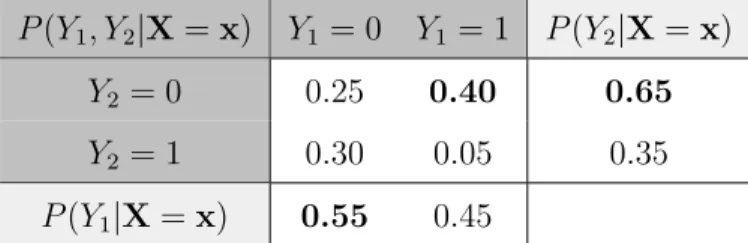
Example 1. Assume the joint conditional distribution of class variables Y1 and Y2 for a
specific instance x is as shown in Table 2.1. The optimal classification for x (according to Equation (2.1)) is h∗(x) = (Y1 = 1, Y2 = 0). However, the result of BR (according to Equation (2.3)) is hBR(x) = (Y1 = 0, Y2 = 0).
P(Y1, Y2|X =x) Y1 = 0 Y1 = 1 P(Y2|X=x)
Y2 = 0 0.25 0.40 0.65
Y2 = 1 0.30 0.05 0.35
P(Y1|X=x) 0.55 0.45
Table 2.1: The joint distribution of class variablesY1 and Y2 conditioned on instance x. The optimal (MAP) prediction is h∗(x) = (Y1 = 1, Y2 = 0).
2.1.2 Early Multi-label Classification Approaches
Realizing the deficiency of BR [Boutell et al., 2004, Clare and King, 2001, Schapire and Singer, 2000] in addressing the MLC problem, several research directions have been proposed to model the relations between the class variables. [Godbole and Sarawagi, 2004] proposed a method that builds two levels of classifiers: The first level classifiers learns to predict values of each class variable using the original features (i.e., the first level is equivalent to BR). The second level learns to predict values of each class variable using the original features and the output of the first level. [Zhang and Zhou, 2007] presented the Multi-Label
bindingk-nearest neighbor with Bayesian inference. A combination of ML-KNN and logistic regression was presented in [Cheng and H¨ullermeier, 2009], where the class proportions of nearest neighbors are used as additional features for the logistic regression classifiers. The limitation of these early approaches is that class dependences are either not modeled at all or modeled in a very limited way.
2.1.3 Output Coding Approaches
An alternative approach to MLC is based on the error-correcting output coding (or simply output coding) approach [Dietterich and Bakiri, 1995]. The idea is to encode the output values into a codeword, learn how to predict the codeword, and then recover the correct output from noisy predictions. A variety of output coding methods have been proposed by utilizing different encoding strategies, such as compressed sensing [Hsu et al., 2009], principal component analysis [Tai and Lin, 2010], and canonical correlation analysis [Zhang and Schneider, 2011]. The state-of-the-art in this approach utilizes a maximum margin formulation that promotes both discriminative and predictable codes [Zhang and Schneider, 2012]. The limitation of output coding methods is that they can only predict the single “best” output for a given input, and they cannot compute probabilities for different input-output pairs.
2.1.4 Classifier Chains and Its Extensions
[Read et al., 2009] introduced the Classifier Chains (CC) method for MLC. The idea is to link different binary classifiers in a chain, such that each classifier incorporates the (0/1) predictions of all preceeding classifiers in the chain as additional features. For example, assume that the order of the class variables in the chain is Y1 < Y2, ... < Yd. To classify a
new instance x, classifier h1 first predicts Y1 = yb1 ∈ {0,1} from x. After that, h2 predicts
Y2 = yb2 using x and the predicted value yb1. By repeating this to Yd along the chain, hi predictsYi =ybi using yb1, ...,byi−1 as additional input features.
The CC method has been extended in several ways. [Zhang and Zhang, 2010] realized that the performance of CC is influenced by the order of class variables in the chain (the
original proposal [Read et al., 2009] orders arbitrarily) and proposed a method that learns such ordering from data. [Zaragoza et al., 2011] explored the unconditioned dependence relations in the output space and constructed chains using the mutual information between the class variables.
The main disadvantage of CC and its extensions [Read et al., 2009, Zhang and Zhang, 2010,Zaragoza et al., 2011] is that they do not perform proper probabilistic inference for clas-sification (i.e., they do not correctly solve Equation (2.1)). Instead, they simply propagate the predictions through the class variables according to the order defined by the chain, which is a greedy mode-seeking heuristic [Dembczynski et al., 2010]. However, such a heuristic may produce incorrect results as we show in the following examples.
Example 2. Consider the conditional distribution in Table 2.1 and assume the order of
the class variables in the chain is Y1 < Y2. CC starts incorrectly by predicting Y1 = 0 and eventually produces the suboptimal prediction (Y1 = 0, Y2 = 1).
[Dembczynski et al., 2010] discussed the suboptimality of CC, which is depicted in the above example, and presented Probabilistic Classifier Chains (PCC) that estimates the entire posterior distribution of the class labels. However, this method has to evaluate exponentially many label configurations, which greatly limits its applicability.
2.1.5 Multi-Label Conditional Random Fields
Another approach for modeling P(Y|X) relies on conditional random fields (CRFs) [ Laf-ferty et al., 2001]. [Ghamrawi and McCallum, 2005] presented a method called Collective Multi-Label with Features classifier (CMLF) that captures label co-occurrences conditioned on features. However, CMLF assumes a fully connected CRF structure which requires a high computational cost. Later, [Shahaf and Guestrin, 2009] and [Bradley and Guestrin, 2010] proposed to learn tractable (low-treewidth) structures of class variables for CRFs us-ing conditional mutual information. More recently, [Pakdaman et al., 2014] used pairwise CRFs to model the class dependences and presented L2-optimization-based structure and parameter learning algorithms. Although the later methods share similarities with our
ap-Figure 2.1: An example MBC [van der Gaag and de Waal, 2006,Bielza et al., 2011] which de-fines the joint probability distribution over three class variables{Y1, Y2, Y3}and four feature variables {X1, X2, X3, X4}.
proach by modeling the conditional dependences inYspace using restricted structures, their optimization of the likelihood of data is computationally more demanding. To alleviate this, CRF-based methods often resort to optimization of a surrogate objective function (e.g., the pseudo-likelihood of data [Pakdaman et al., 2014]) or include specific assumptions (e.g., fea-tures are assumed to be discrete [Ghamrawi and McCallum, 2005]; relevant features for each class are assumed to be known [Shahaf and Guestrin, 2009, Bradley and Guestrin, 2010]), which complicate the application of the methods.
2.1.6 Multi-Dimensional Bayesian Network Classifiers
Multi-dimensional Bayesian network Classifiers (MBC) [van der Gaag and de Waal, 2006,
Bielza et al., 2011, Antonucci et al., 2013] build a generative model P(X,Y) using special Bayesian network structures that assume all class variables are ancestors of all feature vari-ables (see Figure2.1). To facilitate the model, MBC parameterize three sets of arcs between the input and output variables: namely,AY,AX, andAX Y such that AY ⊆ VY× VY are the arcs between the output variables, AX ⊆ VX × VX are the arcs between the input variables and AX Y ⊆ VY × VX are the arcs from the output variables to the input variables, where
VX = {X1, ..., Xm} and VY = {Y1, ..., Yd} respectively denote the sets of input and output
variables. Figure 2.1 shows an example MBC that is defined over three class variables and four feature variables.
differ-ences:
• MBC only handles discrete features and, thus, all features should be a priori discretized; while our approach handles both continuous and discrete features.
• MBC defines a joint distribution over both feature and class variables and the search space of the model increases with the input dimensionality m; while our search space does not depend on m.
• Feature selection in MBC is done explicitly by learning the individual relationships be-tween features and class variables; while we perform feature selection by regularizing the base classifiers.
• MBC requires expensive marginalization to obtain class conditional distributionP(Y|X); while we directly model and estimate P(Y|X).
2.1.7 Ensemble Approaches
Several researchers proposed to use the ensemble approach for MLC in order to overcome the limitations and disadvantages that individual models have and achieve more precise and robust performance. [Read et al., 2009] presented Ensemble of Classifier Chains (ECC) that simply averages the predictions of multiple randomly structured CC models that are trained on bootstrapped subsets of data. [Zaragoza et al., 2011] followed the same ensemble approach and proposed Ensemble of Bayesian Classifier Chains (EBCC) that combines several chain-structured MBCs, obtained by changing the root node in the chain. [Antonucci et al., 2013] proposed an ensemble of multi-dimensional Bayesian networks combined via simple averaging. Each MBC in the ensemble represents differentY relation (the structures are set a priori and not learned) and all of the networks adopt the na¨ıve Bayes assumption (i.e., features are independent given class labels).
Although these methods significantly improve the predictive accuracy of the base models, they are limited in that the way they diversify the base classifiers heavily relies on random-ization. Also their ensemble predictions are based on simple (uniform) averaging. Unlike these methods, our ensemble approaches learn the base models (both the structures and
parameters of base classifiers) and the mixing coefficients of the ensemble from data in a principled way.
2.1.8 Our Work
In Chapter 3, we develop and study novel probabilistic approaches that model and predict multi-label data with multivariate responses.
• First, we present a new model that represents the posterior distribution of multivariate responses (class labels) P(Y|X) using tree-structured Bayesian networks [Batal et al., 2013]. By restricting the conditional dependence relations between class variables to follow a directed tree, we devise efficient structure and parameter learning algorithms and a linear time (O(d)) exact MAP inference algorithm.
• Second, we build an ensemble method that incorporates multiple tree-structured Bayesian networks [Batal et al., 2013] into a data model that represents the joint conditional prob-ability P(Y|X) [Hong et al., 2014]. Our approach is based on the Mixtures-of-Trees [Meil˘a and Jordan, 2000] framework that originally defines a generative model of P(Y) for discrete multi-dimensional domains. We extend the Mixtures-of-Trees framework and present efficient supporting algorithms that learn the structures and parameters of the mixture model and perform a fast MAP inference for MLC.
• Last, we improve our ensemble method [Hong et al., 2014] by developing a generalized mixture framework for MLC [Hong et al., 2015]. We first propose a generalized repre-sentation of the class posterior distribution P(Y|X) that includes a number of previous MLC models [Boutell et al., 2004, Clare and King, 2001, Batal et al., 2013, Read et al., 2009] as special cases. We then extend the Mixtures-of-Experts [Jacobs et al., 1991] framework, which was originally built for the conditional distributionP(Y|X) such that, by using our generalized class posterior models as base classifiers, the framework repre-sents the joint conditional distribution. Our mixture representation recovers a rich set of dependence relations among inputs and outputs that a single MLC model cannot capture due to its modeling simplifications.
2.2 CONDITIONAL OUTLIER DETECTION
This section considers the conditional outlier detection problem in (possibly high-dimensional) binary response space – which we refer to as theconditional outlier detection(COD) problem. Conditional outlier detection is a special type of the outlier detection problem where data consists of m-dimensional continuous input vectors (context attributes) and corresponding
d-dimensional binary output vectors (response attributes). Our goal is to precisely identify the instances with unusual input-output associations. Following the definition of an out-lier given by Hawkins [Hawkins, 1980],1 we define multivariate conditional outlier in plain
language as follows:
Definition 1. A multivariate conditional outlier is an observation, which consists of context
and associated responses, whose responses are deviating so much from the others in similar contexts as to arouse suspicions that it was generated by a different response mechanism. As we illustrated in Chapter 1, this definition of conditional outlier fits well with various practical outlier detection problems that require contextual understanding of data.
However, the majority of existing methods are designed only to detect unconditional outliers that correspond to unusual data patterns expressed in the joint space of all data at-tributes. Apparently, these methods do not consider the dependences among the attributes and are not able to properly detect conditional outliers. Although there are several con-ditional outlier detection approaches that attempt to recover and reflect the input-output relations for outlier detection, existing solutions are rather limited and not capable of han-dling the particular problem that we are interested in. Below we briefly review existing outlier detection research, discuss their limitations in solving the multivariate conditional outlier detection problem in detail, and differentiate our multivariate conditional approach to them.
1While the concept of outlier is rather ill-defined and, indeed, there is no clear consensus on what an
outlier is, probably the most referenced definition has been given by [Hawkins, 1980]: “An outlier is an observation deviating so much from the others as to arouse suspicions that it was generated by a different mechanism.”
2.2.1 Unconditional Outlier Detection Approaches
One of the most important components in outlier detection research is the assumption regard-ing how outliers occur in a dataset. Below we categorize existregard-ing unconditional outlier de-tection approaches intosix general groups (according to the assumption that the approaches have: distance-based, density-based, depth-based, deviation-based, classification-based, and high-dimensional approaches), and summarize their main ideas.
2.2.1.1 Distance-based Approaches Distance-based approaches are one of the
com-monly used unconditional outlier detection approaches. The methods that fall in this cat-egory assume that normal data instances are located in or near the main body of data distribution, while outliers are found far away from most data instances. Several parametric and nonparametric methods are proposed based on this assumption. Typical parametric examples are [Rousseeuw and Hubert, 2011,Rousseeuw and Zomeren, 1990,Rousseeuw and Leroy, 1987] that assign each data instance an outlier score using a robust distance metric ([Hubert and Debruyne, 2010, Rousseeuw and Driessen, 1999, Rousseeuw, 1984]) between each instance to the distribution center (e.g., mean or median).
The nonparametric methods in this category have been proposed to evaluate outlier scores by analyzing the distance to the local neighbors of each data instance. [Knorr and Ng, 1997] computes the outlier score by counting the number of neighboring instances within a hypersphere of radius d. An instance is considered as an outlier if more than a fraction
α of its k nearest neighbors are further thand from it. Similarly, [Byers and Raftery, 1998] and [Guttormsson et al., 1999] evaluate the outlier score of an instance using the distance to its k-th nearest neighbor in the dataset. [Eskin et al., 2002, Angiulli and Pizzuti, 2002] extend the preceding methods to replace the outlier score with the sum of the distances to the k nearest neighbors.
The distance-based approaches have been very popular in many applications as they are easy and flexible. In particular, the nonparametric methods in this category are flexible with respect to different data types in that they do not make assumptions about the underlying data distribution and can adapt by replacing the distance metric. However, the approaches
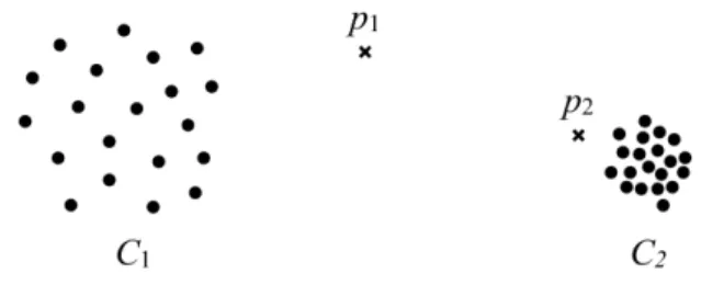
Figure 2.2: Example where the use of local density is desired.
are often computationally very demanding as they require to compute the distance between every instance pairs. Moreover, coming up with a proper distance metric is difficult when the data type is mixed or complex, such as graphs and sequences. Lastly, the approaches suffer from the “curse of dimensionality” issue [Weber et al., 1998,Hinneburg et al., 2000,Aggarwal et al., 2001]; i.e., as the dimensionality of data increases, the distance metrics and density estimators become analytically ineffective and computationally intractable. These make the methods less suitable for high-dimensional data.
2.2.1.2 Density-based Approaches Another category of widely used outlier detection
approaches is the density-based approaches. This category of methods assumes that the density around a normal data instance is similar to the density around its neighbors while that of an outlier is relatively lower than its neighbors. This assumption is particularly useful in many real-world application where the data has regions of varying densities. For example, in the dataset shown in Figure 2.2, the clusters C1 and C2 have different densities whereas the instances p1 and p2 are outliers that we want to identify. With the distance-based approaches, onlyp1 can be identified as an outlier because, for any instance inC1, the distance between the instance and its nearest neighbor is greater than the distance between
p2 and C2. In other words, p2 would be considered as an outlier, only after all instances in
C2 are considered as outliers.
A number of nonparametric methods have been proposed to tackle the above illustrated issue by estimating local density. Local Outlier Factor (LOF) [Breunig et al., 2000] is one of the most popular methods in this regard. LOF evaluates the outlier score of a data instance
Figure 2.3: Difference between the neighborhoods used by LOF and COF (whenk = 6).
by computing the ratio between the local density of the instance and the average local density of k neighboring instances: LOF (x, k) = P x0∈N k(x) lrdk(x0) lrdk(x) |Nk(x)|
where Nk(x) denotes thek-nearest neighborhood of instance x and
lrdk(x0) = |Nk(x0)| P x00∈N k(x0)max(k-dist(x 00),dist(x0,x00))
is the local reachability density, which in essence measures the geometric dispersion of the
k-nearest neighborhood. The score given by LOF can be understood as the inverse of the relative density within the local neighborhood. Instances that have LOF score greater than 1 are generally considered as outliers.
LOF has influenced several subsequent works in the literature. For instance, Connectivity-based Outlier Factor (COF) extends LOF [Tang et al., 2002] to detect outliers from data on a manifold. The key difference of COF in contrast to LOF is how the method defines the local neighborhood. Specifically, to find theknearest neighbors of an instancex, COF incre-mentally grows a neighbor set denoted as N0(x): First off, COF adds the nearest neighbor of x to N0(x). Then, COF repeatedly finds and adds other neighboring instances to N0(x) until |N0(x)| = k, such that the newly added instance has the smallest distance to any of the previously added instances in N0(x). Unlike LOF, COF can capture localities over line components as compared in Figure 2.3.
Figure 2.4: An example multi-granularity problem.
[Papadimitriou et al., 2003] propose another variants of LOF, called Local Correlation Integral (LOCI), to address the granularity problem in outlier detection. The multi-granularity problem refers to a case where data is polluted not only from outlier instances but also from outlying-clusters (groups of outliers; see Figure2.4). LOF is not able to handle such a problem unless a proper value of the neighborhood sizek is provided. LOCI addresses it by introducing Multi-Granularity Deviation Factor (MDEF) that, for each test instance, computes the standard deviation of the local densities of the nearest neighbors. The outlier score of the instance is assigned by taking the inverse of this standard deviation.
The unique advantage of the density-based approaches is in that the solutions can be locally sensitive, which in turn let the approaches achieve a better detection accuracy in many real-world applications. The approaches are also very flexible as they do not make assumptions about the underlying data distribution. However, similar to the distance-based approaches, the density-based approaches are not easily scalable to larger datasets, because the solutions require a pairwise distance matrix to find neighborhoods. In addition, some-times a proper distance metric cannot be easily determined, which may limit the applicability of the approaches. Lastly, as with the distance-based approaches, the approaches also suffer from the “curse of dimensionality” issue [Weber et al., 1998,Hinneburg et al., 2000,Aggarwal et al., 2001].
(a) Dataset (b) Depth assigned by convex hull analysis
Figure 2.5: Depth-based outlier detection.
2.2.1.3 Depth-based Approaches Depth-based approaches assume that normal data
instances are close to or in the center of data clusters, whereas outliers are at the fringes. Several nonparametric methods fall in this category that assign each data instance a depth
k by gradually removing data using iterative convex hull analysis (Figure 2.5). At each iteration, all points that lie on the convex hull of data instances are removed; a depth ofk is assigned to the removed instances. The instances with a low depth are considered as “fringe” instances and are possible candidates for outliers [Ruts and Rousseeuw, 1996,Johnson et al., 1998].
The approaches are flexible in that no assumption regarding the underlying data distri-bution is required. However, an application of the approaches could be very limited due to the computational cost of the convex hull analysis (usually only efficient with low dimen-sional datasets). Also, a convex hull ind-dimensional space contains at least 2dpoints, which
induces a large portion of data to be considered as outliers. This makes the approaches in high-dimensional spaces extremely ineffective.
2.2.1.4 Deviation-based Approaches Deviation-based approaches assume outliers are
the outermost instances in a dataset, such that a removal of an outlier lowers the variance of the set to a large extent. One of the well-known nonparametric methods in this category is Linear Method for Deviation Detection (LMDD) [Arning et al., 1996]. Given a dataset, the method computes how much the variance is reduced (called smoothing factor) by removing
(a) Multi-class strategy (b) One-class strategy
Figure 2.6: Classification-based outlier detection.
an instance. The instances whose exclusion minimizes the variance are treated as outliers. As with other nonparametric methods, the deviation-based approaches do not require an assumption with respect to the underlying data distribution. However, the approaches require O(2n) times of variance estimation, which limits the application of the approaches. That is, for a dataset of size n, there are 2n options of which instances to remove, which
makes the approaches less scalable to large datasets.
2.2.1.5 Classification-based Approaches Classification-based approaches are based
on a parametric assumption that a function of feature classifying normal and outlier instances can be learned from data. There are two major strategies to achieve classification-based outlier detection: multi-class and one-class classification strategies.
Multi-class classification strategy further assumes that normal data instances form a set of clusters (that the cluster information is either provided as class labels, or discovered by an additional clustering step). It then learns a classifier for each cluster in the one-vs-all manner.2 In the testing time (when detecting outliers using the learned classifier),
instances that do not belong to any of the clusters are considered to be outliers. Many early methods are developed based on this strategy. [De Stefano et al., 2000, Odin and Addison,
2For each data cluster, a classifier is trained by treating the cluster as the positive class and the other