Washington University in St. Louis
Washington University Open Scholarship
Doctor of Business Administration Dissertations Olin Business School
Spring 5-2019
Machine Learning and Empirical Asset Pricing
Yingnan Yi
Follow this and additional works at:https://openscholarship.wustl.edu/dba
Part of theBusiness Administration, Management, and Operations Commons, and theFinance and Financial Management Commons
This Dissertation is brought to you for free and open access by the Olin Business School at Washington University Open Scholarship. It has been accepted for inclusion in Doctor of Business Administration Dissertations by an authorized administrator of Washington University Open Scholarship. For more information, please [email protected].
Recommended Citation
Yi, Yingnan, "Machine Learning and Empirical Asset Pricing" (2019).Doctor of Business Administration Dissertations. 7.
Machine Learning and Empirical Asset Pricing
Yingnan, Yi
∗ Current Draft: May 6, 2019Abstract
In this paper, I conduct a comprehensive study of using machine learning tools to fore-cast the U.S. stock returns. I use three sets of predictors: the past history summarized by 120 lagged returns, the technical indicators measured by 120 moving average trading signals, and the 79 firm fundamentals, which helps to understand the weak-form market efficiency, algorithm trading and fundamental analysis. I find each set independently has strong predictive power, and buying the top 20% stocks with the greatest predicted returns and shorting bottom 20% with the lowest earns economically significant profits, and the profitability is robust to a number of controls. Econometrically, neural network generally improves forecasting over linear models, but makes little difference with firm fundamental predictors. Ensemble method tends to perform the best. However, when combining information from all the predictors, traditional machine learning improves little the performance due to perhaps not enough time series for too large dimensional-ity. In contrast, simple forecasting combination and portfolio diversification approach provide large gains.
Keywords: Momentum, Machine Learning, Ensemble Learning, Neural Network, Deep Learn-ing.
∗Yingnan Yi is a DBA candidate at Washington University in St. Louis, Missouri, United States §I benefit a great deal from discussions with my advisor Professor Guofu Zhou at Washington University
in St. Louis, Professor Fuwei Jiang at School of Finance of Central University of Finance and Economics, Professor Guohao Tang at Hunan University in China, Dr. Xiaming Zeng at Barclays Capital London Office. All errors are mine
kI gratefully acknowledge the computing support from the Center for High Performance Computing at
Washington University in St. Louis. All computations were performed using the facilities of the Washington University Center for High Performance Computing, which were partially provided through grant NCRR 1S10RR022984-01A1.
1.
Introduction
Machine learning is receiving increasing attention in various areas, i.e., Heaton, Polson, Witte (2016). Recent studies on U.S. market focus on cross-section predictability of stock returns. For example, McLean and Pontiff (2015) examine various anomalies, and Green, Hand, Zhang (2017) examine the predictive power of firm characteristics. The recent study of Han, He, Rapach, Zhou (2018) use machine learning tools to uncover more stable and greater predictability than previously found. Instead of cross-section predictability, Gu, Kelly, Xiu (2018) apply comprehensive set of machine learning tools to study time series predictability. In this paper, I use a comprehensive set of machine learning techniques to analyze cross-sectional predictability of U.S. data over 40-year time period from January 1978 to December 2017. I categorize an extended panel of predictors into three subcategories of different eco-nomic nature and attempt to speak to different questions under machine learning framework. Specifically, I investigate the portfolio performance using: (1) 120 historical monthly stock returns, (2) 120 technical moving average trading signals (Neely, Rapach, Tu, Zhou (2014)), and (3) 79 fundamental firm characteristics. I also compare model performance during sub-periods, by long- and short-leg portfolios, by size quintiles, and during different investor sentiment periods and business cycles. Following Gu, Kelly, Xiu (2018), I apply major ma-chine learning tools available, including ridge, lasso, elastic net, and 5 neural network models of various architectures. In addition, I apply two commonly used dimensionality-reduction techniques, namely principal component regression (PCR) and partial least square (PLS).
To predict stock return during month t using a given model, I estimate the model on data during month t-1 (training sample). I use 5-fold cross validation or a single holdout
validation sample to determine the optimal hyper-parameters or optimal stopping point.1.
The resulting model is used to predict cross-sectional stock return on the data over month t (testing sample). I independently sort stocks into quintiles based on the predicted return
from each model and equal weight stocks within each quintile. The spread portfolio is
constructed by buying the predicted winner quintile and selling the predicted loser quintile. In addition to forming portfolios based on individual models, I construct three ensemble portfolios based on unanimous voting rule. First I split models into two categories: linear and neural network, where linear family includes OLS, PCR, PLS, Ridge, Lasso, and Elastic Net and neural network family includes 5 neural network models with assorted architectures. At the beginning of each month, each estimated model in a given family casts its votes as to in which quintile the stocks will fall in the coming month. Only stocks that receive unanimous votes of top or bottom quintile from all models within a family will be bought or sold. I also
construct a ”total ensemble” portfolio consisting of all 11 models under unanimous voting rule.
Among single-model-based portfolios, our finding shows that in general neural network portfolios perform better than linear ones mainly for price-related predictors, i.e., lagged return and moving average trading signals. For the 120 lagged return setting, the monthly excess return of spread portfolios based on linear models generally falls around 0.8% while the return based on neural networks falls between 0.85% and 1.03%. In addition, combination of linear models (networks) yields monthly return of 1.24% and 1.59%, which are significantly higher than that of any component model in their respective class and represents a 28% (1.59/1.24-1) performance gap between the two classes of models. For the moving average signal setting, the monthly excess return of spread portfolios based on linear models falls around 0.8% while the return based on neural networks falls around 1.0%, about a quarter higher. Like in lagged return setting, combination of linear models (networks) yields monthly return of 1.09% (1.48%), which are approximately 36% (48%) higher than any component model in their respective class and represents a 0.36% (1.48/1.09-1) gap in relative sense. In addition, I observe a significant jump in excess return when linear and networks models are combined. For example, return jumps to 1.74% (from 1.59%) in lagged return setting and to 1.89% (from 1.48%) in moving average signal setting. Risk-adjustment does not weaken our finding.
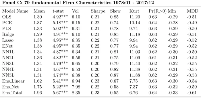
For fundamental firm characteristics, our results show marginal improvement of neural network models over linear models. Monthly excess return of spread portfolios based on linear models falls between 1.29% to 1.38% while return based on neural networks falls between 1.31% and 1.36%, essentially identical to each other. In addition, combination of linear models yields a monthly return of 1.62% while combination of networks yields a return of 1.75%, again close to each other. Nonetheless, such combination still brings significant boost to excess return relative to the return based on individual models. Furthermore, when linear and network models are combined, return jumps to 1.96%, the highest among all models. However, I only observe improvement in Sharpe ratio in the moving average trading signal setting and not in the other two.
Our finding has two implications. First, the success of neural network in our two price-related settings suggests that the true data generating process underlying the follow-the-trend strategy has significant non-linear component. For example, momentum strategy ranks stocks based return history and buy previous winners and sell previous losers. Such strategy assumes linear influence from past returns and is unnecessarily stringent. Our result suggests that relaxing such assumptions may improve predictive performance of momentum strategy. Our finding also suggests that using models with higher capacity and ensemble methods on
market data may provide additional insights into the weak form of efficient market hypoth-esis. Furthermore, unlike traditional momentum strategy which mainly rely on time-series dependence to pick stocks, our design rely on a cross-sectional design and show that the cross-section of prior returns is also informative.
Second, ensemble method, i.e., unanimous votes, boosts predictive power for both linear and neural network models. I propose two explanations. First, considerable amount of noise
exists in predictions from a single model2 and therefore consensus across models help correct
mistakes made by any individual model. It is also possible that I can only approximate part of the true data generating process with any individual model, making it necessary to
combine multiple models to finish the puzzle.3.
Third, I provide evidence that blindly applying neural network models may not be pro-ductive. The effectiveness of neural network largely depends on the data in question. In particular, the weak improvement of neural network over linear models on fundamentals suggests that the information in fundamental data may not be sufficiently complicate to warrant models of high capacity. In such case, linear models suffice and complicate models harm predictibility.
I contribute to several streams of literature. First, our paper relates to a growing body of research on the application of machine learning techniques to financial data. A broad range of previous studies on machine learning techniques focuses on extracting factors from a myriad of predictors and correcting the bias in existing methods. Rapach, Strauss, Zhou (2013) uses Lasso to forecast international equity returns using cross-country lagged returns. Rapach, Strauss, Tu, Zhou (2018) use a second-stage OLS to correct for the downward bias in the first-stage Lasso estimation. Rapach, Zhou (2019) use Sparse-PCA to shrink more weights of principal components to zero to enhance interpretability of principal components
in forecasting stock return. Freyberger, Neuhierl, Weber (2019) and Feng, Giglio, Xiu
(2019) use modified Lasso to select important return predictors from a predictor zoo and to forecast expected stock returns. Light, Maslov, Rytchkov (2017) propose the PLS approach for estimating expected returns on individual stocks from cross-sectional firm characteristics. They start off by modifying the time series PLS adopted by Kelly, Pruitt (2015), and Huang, Chen, Liu (2015) and significantly improve predictive power of firm characteristics. More recently, researchers start to introduce more flexible models to tackle the forecasting task in finance. Butaru, Chen, Clark, Das, Lo (2016) and Sirignano, Sadhwani, Giesecke (2018) apply regression tree and deep neural network to forecast default probability of consumer
2Even after I average predictions from the same neural network architecture across 100 random weight initializations.
3An analogy is the approximation of a function by its Taylor expansion and I use different models to estimate each terms.
credit card and mortgage loans respectively and show great potential of machine learning techniques in risk management. Heaton, Polson, Witte (2016) introduce a general frame work for deep learning in finance and use auto-encoder to reduce the number of stocks used to replicate NASDAQ Biotechnology Index. Gu, Kelly, Xiu (2018) apply machine learning methods to predict cross-sectional stock returns using a broad set of firm characteristics and show great potential of neural network in financial world. I take one step further and try to measure the informational content of predictors of differential economic nature using machine learning techniques.
Second, our study contributes to the momentum and algorithmic trading literature. Prior returns and price/volume-related signals have the potential to generalize to algorithmic or high frequency trading context due to abundance of data. Plenty studies exist in such area. Huang, Zhang, Zhou, Zhu (2019) combine price and fundamental momentum and construct a twin-momentum portfolio which is more profitable than simple summation of the two momentum portfolios. Another study by Han, Zhou, Zhu (2016) simultaneously consider information in moving average prices over short-, intermediate-, and long-horizon and also identify significantly stronger predictive power and lower risk. I extend these research by applying machine learning tools to an expanded set of momentum and price-related predic-tors. I create a panel of 120 prior returns and 120 price/volume trading signals and use machine learning tools to forecast returns on the two datasets independently. Our results challenge weak form market efficiency and shows great potential for algorithmic and high frequency trading with machine learning tools. Third, by separating fundamental variables from others I independently examine machine learning’s applicability to fundamental anal-ysis. I start from the 94 firm characteristics in Green, Hand, Zhang (2017) and exclude 15 price/volume-related predictors to isolate the predictability of fundamental variables. Our results show that simple neural network models do not outperform linear models on funda-mental variables.
The remainder of this paper is organized as follows. Section 2 discusses the design of our tests. Section 3 explains the specification of the models and discusses our selection of hyper-parameters. Section 4 discusses data. Section 5 reports results. Section 6 concludes the paper.
2.
Design
In this section I describe the predictors, loss function, data splitting, hyper-parameter
tuning, and portfolio construction which apply to all models4. Details of models will be
presented in section 3.
2.1.
Predictors
Our target variable is one-month ahead cross-sectional monthly excess returns. I use three sets of predictors and compare their predictive performance using linear and neural network models separately. Our predictors include: (1) 120-month lagged monthly excess return on security level, (2) 60 stock price and 60 trading volume moving average signals (Neely, Rapach, Tu, Zhou (2014)), and (3) 79 fundamental firm characteristics. Since lagged returns are self-explanatory, I explain price/trading volume moving average signals and 79 fundamental firm characteristics in details below.
Following a similar vein in Neely, Rapach, Tu, Zhou (2014), I construct the price and trading volume moving average signals by comparing short-term moving average of monthly closing price and trading volume with their respective long-term moving average. Higher short-term than long-term moving average is interpreted as a buy signal, vice versa for sell signal. Specifically, I calculate the ratio of the short-term and long-term moving average of the two variables and interpret a ratio higher than 1 as a buy signal and a ratio less than 1 as a sell signal. To calculate the price signals, I compute the following:
Si,t = M As,t M Al,t , (1) where M Aj,t = 1j Pj −1
i=0Pt−i for j = s, l, and Pt is month-end closing price. s = 1,2,3 and
l = 6,12,18, ...,120 and therefore I have 60 combinations of short- and long-term comparisons and hence 60 moving average price signals.
For trading volume, I follow Granville (1963) and Neely, Rapach, Tu, Zhou (2014) and first calculate the ”on-balance” trading volume as follows:
OBVt= t
X
k=1
V OLkDk, (2)
where V OLk is trading volume during month k and Dk is a binary variable that takes the
value of 1 if Pk > Pk−1 and -1 otherwise. Then the moving average signals are constructed
using OBV and in the same manner as moving average price signals. Specifically, I compute the following: Si,t = M AOBV s,t M AOBV l,t , (3) where M AOBV j,t = 1 j Pj−1
1,2,3 and l = 6,12,18, ...,120 and again I have 60 combinations of short- and long-term
comparisons and hence 60 OBV moving average signals. I bundle the 60 price and 60
trading volume moving average signals and form the second set of predictors.
To obtain the 79 firm fundamental characteristics, I start from the 102 fundamental char-acteristics in table 1 in Green, Hand, Zhang (2017) and exclude 17 price-, trading volume-, or return-related variables, which are chmom (change in 6-month momentum), indmom (industry momentum), maxret (maximum daily return), mom12m (12-month momentum), mom1m (1-month momentum), mom36m (36-month momentum), mom6m (6-month mo-mentum), std dolvol (volatility of liquidity (dollar trading volume)), retvol (return volatil-ity), std turn (volatility of liquidity (share turnover)), baspread (bid-ask spread), chcsho (change in shares outstanding), pricedelay (price delay), idiovol (idiosyncratic return volatil-ity), ill (illiquidvolatil-ity), turn (share turnover), and zerotrade (zero trading days). I remove these variables to minimize the overlap of information content with lagged return or moving av-erage signals. In addition, I exclude 6 characteristics whose variance inflation factor (VIF) are greater than 7 (due to multicollinearity concern), including betasq (beta squared), dolvol (dollar trading volume), lgr (growth in long-term debt), pchquick (% change in quick ratio),
quick (quick ratio), stdacc (accrual volatility) 5. Therefore, I end up with 79 (102 - 17 - 6)
fundamental characteristics.
2.2.
Loss Function
I employ mean squared error loss function to measure the fitness of our model on the
training set6. On the training set during month t and of size N, the loss value is computed
in equation 4. L(θ)t= 1 N N X i=1 (ri,t−rˆi,t)2, (4)
where ri,t is the monthly stock returns for the ıth firm in month t and ˆri,t is the predicted
returns from model.
2.3.
Data Splitting
To make sure our estimated model generates out-of-sample prediction of stock return ri,t
during month t, I train our model on data during month t-1, Strain,t−1. Strain,t−1 contains
5Per Green, Hand, Zhang (2017), two price-related variables also have VIF greater than 7. They are maxret and mom6m and have already been excluded in the first round of screening
the actual returns during month t-1 as target variable and its aligned (lagged) predictors. Then I use the predictors for month t, which are lagged returns relative to month t, to make predictions. I run a fixed-width rolling window to train our models.
2.4.
Hyper-Parameter Tuning
Many machine learning models involve hyper-parameters that need to be provided before fitting the model. Hyper-parameters are parameters that cannot be estimated directly from the data, including the penalty parameters in Ridge regression and the number of hidden layers and nodes in a neural network. Although there is little theoretical guidance as to how to choose hyper-parameters, the majority of machine learning community endorses the use
of validation sets7.
In this study, I implement either five-fold cross validation or holdout validation to de-termine the optimal hyper-parameter on the validation set. In K-fold cross validation, the training set is first randomly divided into K segments. Then a range of hyper-parametric models are trained on K-1 segments and evaluated on the remaining segment. Each of the K segments takes turns to be evaluated upon and the average loss value on all K segments is assigned as the score of this model. The hyper-parameter that generates the lowest score (loss) are chosen. I apply 5-fold cross validation to PCR, PLS, Lasso, Ridge, and Elastic Net. For neural network, I use a 10% holdout validation sample to pick optimal hyper-parameter.
2.5.
Hedge Portfolios
To construct the hedge portfolio for month t using a specific model, I first train the model on data over month t-1 and select hyper-parameters via cross validation or holdout validation. I use the fitted model to predict stock return during month t. Then I sort the monthly cross-section of stocks into quintiles based on their predicted return and form
equally weighted portfolios for each quintile.8 Finally, I construct the hedge portfolio by
buying the top quintile and selling the bottom quintile. The hedged return is calculated by subtracting the return of the bottom quintile from that of the top quintile.
2.6.
Ensemble Portfolios
I use unanimous voting rule to combine subgroups of models and construct three ensemble portfolios. After training all models, I separate them into linear models and neural networks
7Validation should be combined with domain knowledge whenever available.
8Stocks whose market capitalization as of the end of month t-1 falls below the monthly NYSE 10% breakpoint are excluded from model estimation and prediction.
and construct three ensemble portfolios by combining models within each subgroup and across the two subgroups. Combination is implemented using unanimous voting rule. For each month, I allow models in each subgroup to cast votes on the quintile assignment of stocks for the next month. I then construct ensemble portfolios by buying the unanimously predicted top quintile and selling the unanimously predicted bottom quintile. The spread of return between the top and bottom quintile represents the return to the associated ensemble portfolio. In the rare cases where no unanimous agreement exists during a given month, I simply stop trading and assume that the return for the corresponding leg(s) is zero. The three ensemble portfolios are constructed by combining linear models, 5 neural networks, and all models in our study separately and I name them linear ensemble, network ensemble, and total ensemble in the analysis below.
3.
Models
This sections describes the family of machine learning models used to generate
predic-tions. I provide a brief introduction to each model and its motivation, algorithm, and
parameter tuning, if applicable.
3.1.
Ordinary Linear Regression
The most commonly used model in empirical finance is Ordinary Linear Regression. It serves as a good benchmark for more sophisticated models.
Linear Regression tries to find the β in equation Y = Xβ + that minimize mean
squared prediction errors (MSE). It assumes that the linear regression functionE(Y|X) is a
reasonable approximation of the underlying relation between the target and predictors. For
linear regression to be valid,andY have to be uncorrelated. As long as this condition holds,
the Gauss-Markov Theorem asserts that the ˆβestimated from Ordinary Least Square has the
smallest variance among all linear unbiased estimates, a.k.a. Best Linear Unbiased Estimator or BLUE. Although linear regression allows easy interpretation, it imposes linearity on the underlying relation which limits its predictive power if the true underlying function is other than linear. In addition, OLS typically incurs high variance in predictions when the number of predictors increases because it places no control over the norm of parameters. The generic solution to OLS can be derived through first-order condition on the MSE and its derivation can be found in a classical textbook.
3.2.
Principal Component Regression and Partial Least Square
As the number of predictors increases, the variance of prediction from linear regression increases dramatically. Since each estimated parameter contributes randomness into the prediction, noise accumulates and eventually dominates the true relation between predictors and the target. One method to counter the problem is to reduce the dimension of predictors by extracting latent variables embedded in the predictors. The hope is to represent the information in the original predictors with only a few important hidden components and reduce the dimension of predictors. Two methods are commonly used for this purpose: principal component regression and partial least square regression.
3.2.1. Principal Component Regression
Principal component regression (PCR) is merely a regression of the target variable on the hidden components from principal component analysis (PCA). The first principal com-ponents are found to be the linear combination of the original predictors that has the highest
variance among all such linear combinations. Subsequently, theithprincipal components are
found in the same manner with the additional requirement that they must be orthogonal to all previously found principal components. Mathematically, the principal components of a
data matrix X are given by the eigenvectors of XTX. This is intuitively appealing because
XTX is the variance-covariance matrix of X and its eigenvectors point to the direction in
which the variables inX vary the most9. In optimization term, themth component direction
vm solves equation 5. max α V ar(Xα) subject to ||α||= 1 αTSvl = 0 l= 1, ..., m−1 (5)
where S is the covariance matrix of the data.
In each month, I determine the optimal number of principal components retained using five-fold cross validation. For implementation, I follow the algorithm called ”Non-linear Iter-ative Partial Least Square” , aka ”NIPALS”, which repeatedly calculates every component, checks their convergence, and stops until certain low tolerance level is achieved or maximum
9HereX must be demeaned before performing PCR. The eigenvector associated with the largest eigen-value points to the direction in which the linear combination has the largest variance.
iteration is reached10. See Algorithm 1 in Appendix for details11.
3.2.2. Partial Least Squares Regression
Like principal component regression (PCR), partial least squares (PLS) also construct linear combinations of the original predictors to represent the data. However, PLS improves upon PCR by incorporating the correlation between predictors and the target into the cal-culation of weights in linear combination. That is, PLS finds directions that have both high variance among predictors and high correlation with the target, while PCR only focus on
ex-plaining the variance among predictors. In optimization form, themthPLS component solves
equation 6 whose objective function clearly demonstrates the consideration of correlations between predictors and the target.
max α Corr 2(y, Xα)V ar(Xα) subject to ||α||= 1 αTSvl = 0 l = 1, ..., m−1 (6)
where S is the covariance matrix of the data.
As in PCR, I determine the optimal number of principal components retained using five-fold cross validation. I also follow the NIPALS algorithm as in PCR.
3.3.
Penalized Linear Regression
3.3.1. Ridge Regression
Ridge regression shrinks the norm of the coefficient vector by imposing a penalty term on
the loss function. Specifically, in our study the optimization algorithm finds ˆβ in equation 7.
ˆ
βRidge = arg min β nXN i=1 (yi−β0− p X j=1 xijβj)2+λ p X j=1 βj2o, (7)
where β is the vector of regression coefficients, xij is the jth predictor of the ith training
sample,N is training sample size, andλ≥0 is a penalty parameter that controls the amount
of shrinkage. Larger λimposes more difficulty to the minimization of loss function and thus
shrink theβmore strongly toward zero. Using matrix notation, the Ridge regression solutions
are given in equation 8.
10For our study, the tolerance level is 1e-06 and maximum iteration is 500, whichever comes first. 11NIPALS applies to partial least squares as well with only minor modification.
ˆ
βRidge= (XTX+λI)−1XTy, (8)
where X is data matrix and y is the target variable. The method of penalizing loss
function by the squared norm of β is called L2 regularization and is also used in neural
network models, which will be discussed in later sections.
An important insight can be gathered by performing singular value decomposition of the
centered data matrix X, X = U DVT, where U spans the columns of X, D is the diagonal
matrix of singular values, andV spans the row space. PluggingX =U DVT into equation 8,
left-multiply byX, and simplify to get equation 9.
XβˆRidge = p X j=1 uj d2 j d2 j +λ uTjy, (9)
where uj is the jth column of U, λ is the penalty parameter in equation 7, and .j is the
singular value of X.
Equation 7 shows that Ridge regression proceeds in two steps. First, it computes the
coordinates of y relative to the orthogonal basis U. Then it shrinks these coordinates by
multiplying them with d
2
j
d2
j+λ
. Note that the directions along which the coordinates exhibit
smaller variance receive larger shrinking12. Intuitively, since data does not vary much along
such directions, their effects are more difficult to estimate accurately. As a result, Ridge
regression assigns a lower weights13. The only tuning parameter λ is found by ten-fold
cross-validation.
3.3.2. Lasso Regression
Lasso regression follows a similar spirit as Ridge regression in that Lasso also imposes a
penalty term to the loss function that is a function of theβvector. However, Lasso calculates
the L1 norm while Ridge calculates L2 norm (See equation 10). This modification has two
major implications. First, the absolute value function precludes a close-formed solution as in Ridge regression. Thus the Lasso estimates have to be solved numerically. Second, Lasso
regression tends to shrink someβito zero and thus Lasso can be viewed as a variable selection
method.
12Recall thatd2
jis the eigenvalue ofXTXand eigenvector associated with largerd2j points to the direction
in which data varies the most.
13See ”The Elements of Statistical Learning: Data Mining, Inference, and Prediction” Chapter 3 for more detailed discussions.
ˆ
βLasso = arg min β nXN i=1 (yi−β0− p X j=1 xijβj)2+λ p X j=1 |βj| o , (10)
where all variables are defined similarly as in equation 7 and λ is found by ten-fold
cross-validation.
3.3.3. Elastic Net
Ridge and Lasso regressions can be viewed as two extremes. Ridge regression tends to retain all variables while Lasso performs variable selection. Zou and Hastie (2005) proposed a compromise between the two methods, namely Elastic net, which performs some vari-able selection and in the meanwhile shrinks the coefficients of correlated varivari-ables. This is illustrated in equation 11.
ˆ
βElastic = arg min β nXN i=1 (yi −β0− p X j=1 xijβj)2 +λ p X j=1 (αβj2+ (1−α)|βj|) o , (11)
where all variables are defined similarly as in equation 7 and 10 and λ and α are found by
ten-fold cross-validation as well.
3.4.
Neural Network
Neural network is by far the most powerful tool in machine learning toolkit. Its de-velopment was partly motivated by the failure of traditional algorithms to generalize well to artificial intelligence tasks, i.e., speech and computer vision recognition. As its imple-mentation becomes more user-friendly, neural network has shown great potential in tackling problems in finance, i.e., Gu, Kelly, Xiu (2018). In the following subsections, I go through the building blocks of the neural network and explain our design in details.
3.4.1. Universal Approximation Property
A key property that makes neural network the pivot of machine learning is the universal approximation property. The universal approximation theorem (Hornik (1989), Cybenko (1989)) states that a feed-forward network with a linear output layer and at least one hid-den layer with any squashing activation function (that maps a larger domain into a smaller range, i.e.,sigmoid function) can approximate any Borel-measurable function from one finite-dimensional space to another with any desired nonzero amount of error, provided that the network is given sufficient hidden units. For our mission of predicting stock returns with
lagged return, moving average price/trading volume signals, or firm fundamentals, I can safely assume that all of our predictors are bounded during a specific time period and univer-sal approximation theorem applies. Take lagged return for example, univeruniver-sal approximation
theorem implies that any continuous function f : [−1,1]n → [−1,1] may be approximated
by a neural network with large enough capacity, wheren is the number of predictors.14. The
other two settings can be similarly argued.
3.4.2. General Architecture of the Network and Information Flow
Although universal approximation theorem guarantees the existence of a large enough
network 15 that approximates any Borel-measurable function with any degree of accuracy,
the number of hidden nodes in the single-layer network may be too large to be estimated
Barron (1993). In practice, the architecture of a network is more often determined by
experimentation. Figure 1 shows a general structure of neural network with five input nodes (predictors), one hidden layer with three hidden nodes (latent features), and one output
node (predicted stock return) 16.
Fig. 1. General Architecture of a Neural Network
Input layer Hidden layer Output layer Input 1 Input 2 Input 3 Input 4 Input 5 Ouput
14Recall that continuous function on a closed bounded subset of
Rn, i.e., compact, is Borel-measurable and [−1,1]nand [−1,1] are obviously finite dimensional∀n <∞. Thus the conditions of universal approximation
theorem are satisfied.
15In the sense of sufficient number of hidden nodes in a single hidden layer
16Figure 1 and figure 2 are adapted from the open source codes on
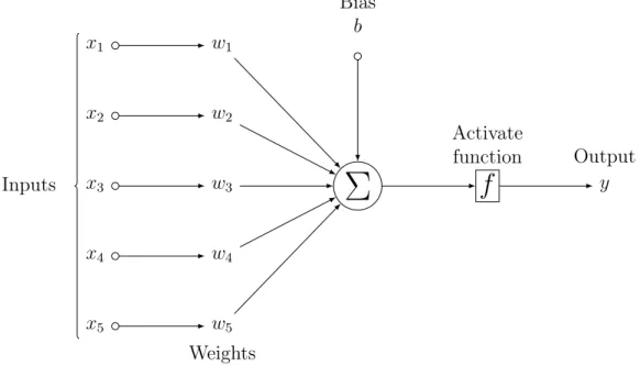
Zooming in to a specific node in the structure in Figure 1, I obtain a more microscopic view of the information flow within the structure for a single hidden node. Figure 2 shows the mechanics and I briefly introduce the process. First, I take a single observation with five inputs (predictors) and then apply a weighted average on the inputs using weights
w1, w2, w3, w4, w5 (to be estimated from training) to obtain the summationP
. Second, add
a bias parameter b to the P
. So far the procedure resembles regression analysis. Finally, I apply an activation function to the resulting value from previous step and pass the output to following layer, i.e, another hidden layer or output layer. The key point is that all the weights and biases are parameters I try to estimate and all other parts, i.e., hidden layers and nodes, activation functions, penalty terms, regularizations (not shown in the graph) are pre-chosen. I will explain these issues and our choices momentarily. Before that, a more fundamental task is to initialize weights and biases and then to update them, which leads us to weight initialization, forward and backward propagation, and stochastic gradient descent.
Fig. 2. Information Flow Through One Hidden Node of a Feed-forward Network
x3 w3
Σ
f
Activate function y Output x1 w1 x2 w2 x4 w4 x5 w5 Weights Bias b Inputs 3.4.3. Weight InitializationMost optimization algorithms used in training neural networks are iterative in nature and require initial point to start. Initial point has three vital implications. First, most optimization algorithm for neural networks are strongly affected by initial points, i.e., it affects whether iteration converges at all. Second, even if learning does converge, initial
point affects the convergence speed and training time. Third, although different initial points can sometimes converge to points of comparable cost value, these points may have drastically different generalization power. Although these issues are conceptually important, practical strategies are mostly heuristic because neural network optimization itself is not well understood yet.
Glorot, Bengio (2010) shows that for information to flow stably through the network the variance of the outputs of each layer should equal to the variance of its inputs, which is
impossible unless ninputs = noutputs. As a compromise, I use a popular distribution named
”He normal” (He, Zhang, Ren, Sun (2015)) to initialize the weights. This modified normal distribution has been shown to work well with Rectifier Linear Unit (ReLU) activation function and its known variants which I use. Specifically, the initial weights are randomly sampled from the following normal distribution.
X ∼ N(0,√2
s
2
ninputs+noutputs
) (12)
, whereninputs is the number of inputs nodes and noutputs for outputs. Note that this
distri-bution is also intuitively appealing because as the number of inputs and outputs increases, the initial weights are shrunk to zero to dampen the impact of any individual predictor.
3.4.4. Forward- and Backward-Propagation
After the weights are initialized, I iteratively update them using information from the calculated cost value. The two processes of propagating information forward through the neural network and then using calculated errors to make backward adjustments to parameters are called forward- and backward-propagation respectively. Specifically, given the weights matrices and bias parameters of the model, forward-propagation processes the data and
calculate the loss value 17. Then backward-propagation will calculate the gradients on the
activation functions in each layer, starting from the output layer and going backwards to the very first hidden layer. These gradients indicate in which direction the output of each hidden layer should move to reduce the forecast error. Finally, the gradients on weights and biases can be found through chain rule of calculus. (see Algorithm 3 in Appendix for more details)
In practice, the gradients are typically calculated in mini-batches of 32 to 512 randomly
selected training samples at a time 18, i.e., LeCun, Bottou, Muller (2012). In this case,
17The calculated cost value must be added to a regularizer Ω(ω) to obtain the total loss
18A batch size of 1 is totally legitimate. In that case it is a pure stochastic gradient descent algorithm and it probably takes a long time to train the model
the gradient from each mini-batch is simply the average gradient of all samples from the same mini-batch. The batch size is another hyper-parameter I can play with and it also has significant impact on model performance. While using larger batch size may yield more accurate estimate of the gradient due to the law of large number, it also requires more memory on your machine when data is large. On the other hand, for some structure of the cost function more accurate locally estimated gradient may be undesirable when your model is following a trajectory to get out of a local minima or saddle point while its gradient is
telling it to move downhill 19. In our study, I balance model performance against training
time and choose the batch size of 32.
3.4.5. Stochastic Gradient Descent
The most commonly used optimization algorithm for neural network is stochastic gradient decent (SGD). The central equation for iterative updating of weights is shown in equation 13 (see Algorithm 2 in Appendix for more details).
wt←wt−1−t−1gˆt−1, (13)
wherewtis the weight matrix after thetthiteration,t−1is the learning rate after the (t−1)th
iteration, and ˆgt−1 is the estimated gradient from a mini-batch.
Equation 13 shows that SGD relies on the estimated gradient at a sample point20 as
guidance regarding to which direction the weights should move toward. One drawback of SGD is that convergence may be slow and therefore many modified versions exist to accelerate training. In our study I employ an adaptive learning rate algorithm called ADAM Kingma, Ba (2017). See Algorithm 4 in Appendix for details. ADAM can be roughly viewed as a combination of two adaptive learning rate optimization schemes: (1) momentum, and (2) re-scaling.
Intuitively, momentum represents accumulation of previous estimates of gradients and it will be added to the updating term on weights. With momentum the size of updates will depend on the sum of norms of previous gradient estimates and how aligned their signs are. For example, if the training process experiences a long sequence of either positive or negative gradient estimates then the momentum term will accumulate and the size of updates will be larger over time, shortening the training time. If the signs oscillate and previous gradients cancel out then momentum will be close to zero and the size of updates would be small, elongating the training time.
19In this case, an ”inaccurate” estimate of gradient may lead us to the right path. Thanks to an anonymous discussant on Stackoveflow to point this out.
3.4.6. Hidden Layers and Activation Function
Now that I are clear on how to initialize weights and biases and how to iteratively update them, I come back to our design choices, i.e., number of hidden layers and nodes and choice of activation functions. As demonstrate in Figure 1, hidden layers and nodes act like latent variables between predictors and target variable and much of the flexibility of neural network model comes from its layered design and non-linear activation function. Due to the lack of theoretical guidance, architectures are usually designed by experiments. Following previous studies, Gu, Kelly, Xiu (2018) and Masters (1993), I explore a series of designs starting from the shallowest network with a single hidden layer and 32 hidden nodes to a 5-layer network with [32, 16, 8, 4, 2] hidden nodes respectively. Although these pyramidal designs seem arbitrary, casual experiments suggest that deviation from them does generate inferior predictive performance most of the time.
As for activation function, I choose leaky rectified linear unit (Leaky ReLU) function for hidden layers and linear function for output layer. Leaky ReLU is a variant of the famous rectifier linear unit (ReLU) activation function used in many recent studies. Comparison of the two functions are in Figure 3.
The functional forms of ReLU and Leaky ReLU function are given below. ReLU(x) = 0, if x≤0. x, otherwise. LeakyReLU(x) = αx, if x≤0. x, otherwise.
where α is a hyper-parameter that can be tuned 21.
The major difference between ReLU and Leaky ReLU lies on the negative part. One drawback of the original ReLU function is that if during training a hidden node’s weights get updated such that the weighted average of its inputs is negative, it will output zeros. That is, that node is ”dead”. To make things worse, future updates to that node is unlikely to bring it back to life because the gradient of ReLU function is zero on the negative part
of its domain 22. To alleviate this issue, Leaky ReLU assigns a small positive slope to the
original ReLU on the negative domain and hopes that even if a node dies in one round of training future updates will not always be zero and thus may bring it back to life.
As for output layer, linear activation function is a common choice for regression. Since our target variable is stock return which lies in [-1,1], many other functions with a range
between -1 and 1 seem to be legitimate options as well 23. However, such functions typically
saturates for extreme values on their range and thus may cause trouble for optimization
algorithms 24.
3.4.7. Regularizations
With tens of thousands of parameters estimated, over-fitting is a big concern. Conceptu-ally, over-fitting refers to a situation where the model family not only includes the true data generating process but also many other generating processes. That is, variance rather than bias dominates the estimation error (Goodfellow et al (2014)). This issue is especially severe
21Typical choices ofαis 0.01. In our study, I use α= 0.1. The choice ofαcan potentially affect model performance, a fact I observe from experiments. The consideration is to alleviate the dying node problem while preserving the non-linearity of the original ReLU function. No hard rules exist here.
22Recall that during backward propagation I use calculus chain rule to calculate the gradients on weights and biases. If the gradient of activation function on its input weights is zero, the whole gradient becomes zero and the weights don’t get updated. One direct consequence of dying node is that the neural network model starts to generate identical predictions, which is just the bias parameter.
23For example, tangent hyperbolic function.
24That is, such activation functions level off for extreme input values and thus their gradients are close to zero, providing little information for updating weights.
with neural network because neural network typically has very high capacity25. To address
over-fitting, I employ seven regularization schemes: (1)L1 andL2 parameter norm penalties,
(2) adaptive learning rate shrinkage through stochastic gradient descent, (3) learning rate shrinkage through learning rate scheduler, (4) batch normalization, (5) random dropout, (6) early stopping, and (7) ensemble method. The application of regularization is more of an art than science. Although the seven techniques are very powerful, they impose danger as well. Too much regularization may impose unnecessary constraints on the optimization algorithm
and prevent it from heading for a lower cost point. L1 and L2 parameter norm penalties are
essentially the same as the ones used in Lasso and Ridge regressions respectively and thus are spared from further discussion.
I employ two learning rate shrinking methods, one is embedded in the ADAM algorithm as discussed in 3.4.5 and the other is an explicit scheduler. Although ADAM adaptively shrinks learning rate there is little guarantee that the learning rate will be sufficiently shrunk before the early stopping criterion is met. Large learning rate can cause the weights to oscillate back and forth around a local minima and make it difficult to converge. This issue is especially severe during later phase of training when fine tuning is needed. By imposing an explicit learning rate scheduler, I put a shrinking series of upper limits on the learning rates computed
by ADAM at a given step of training and thus make sure that the updating term t−1gˆt−1
in equation 13 will converge to zero and thus the training will converge26.
Batch normalization (Ioffe, Szegedy (2015)) controls the variability of predictors across different layers of the network and across different datasets. The outputs of a mini-batch of data from each layer constitute a ”batch”. The outputs from preceding layers are cross-sectionally standardized to have zero mean and unity variance before being fed to the next layer. This is done on training and validation samples similarly and on testing sample but in a different manner. To make prediction, I treat the entire testing sample as one batch and
feed it to the model in its entirety.27. That is, the mean and variance used in normalization
is calculated using all the data points in a testing sample.
Dropout (Srivastava et al (2014)) randomly ignores a certain percentage of hidden units during training. All the inputs and outputs connected with the ignored units are omitted from updates as well. Since I use a minibatch-based learning algorithm, units to be ignored are chosen at the beginning of each batch operation and they are chosen independently for
25Meaning they include many data generating processes besides the true one, if at all.
26As discussed in Deep Learning Chapter 8 by Ian Goodfellow and Yoshua Bengio, gradient descent often does not arrive at any critical point, meaning that the norm of the gradient does not converge to zero at all. As a result, I must shrink learning rate instead to achieve convergence.
27As discussed earlier, during training and validating I feed a mini-batch of 32 data points to the model at one time. Batch normalization is performed on this mini-batch of 32 examples during training and validating.
each hidden layer. Conceptually, random dropout is similar to estimating an ensemble of sub-networks of the master network with shared parameters. Predictions are made from accumulating votes from all the sub-networks. Like bagging, such ensemble approach has the advantage of being robust to errors. In addition, since dropout is applied on hidden units rather than the raw inputs, it can be viewed as an intentional omission of some information content rather than the original variable from the learning process. This omission forces the algorithm to complete the task via other useful information in the predictors and to extract as much information from the predictors as possible. In our study, the probability of a hidden node being ignores is set at 10%. No dropout is performed on input layer.
Early stopping is a direct control of model performance on the validation set. Typically, I observe that validation loss first decreases with more updates to the weights and then increases as over-fitting creeps in. One way to choose the optimal hyper-parameters is to train the model for a large number of epochs and then go back along the training history to choose the parameters yielding the lowest validation error. However, such method is time consuming and it is difficult to determine how long the entire training process needs to be to include the true optimal model. Instead, early stopping halts the training as soon as the validation error fails to decrease for a certain number of training rounds. At the end of the training process, the most recently recorded model, rather than the global optimal model trained so far, is returned. In our study, I stop the training if the validation error fails to decrease within 10 epochs. See Algorithm 6 in Appendix for details.
Ensemble learning estimates the same neural network architecture multiple times and averages their predictions. Since each estimation assumes a random matrix of initial weights, it incurs independent estimation error, which supposedly will average away with large number of estimations. For each month, I estimate each neural network 100 times using randomly initialized weight matrices and take average prediction as our final prediction.
4.
Data
Market return is collected from monthly CRSP database. Data starts in January 1978 (1978:01) and ends in December 2017 (2017:12), totalling 40 years (480 months). I include all domestic common stocks listed on the NYSE, AMEX, and Nasdaq Stock Exchanges and exclude securities that do not have CRSP share code of 10 or 11. Returns are adjusted by de-listing returns and and stock prices are adjusted by stock dividends and splits. For the 120 lagged returns setting, I require a firm-month to have non-missing past returns for at least 72 months out of 120 months to be included in our sample. For the 60 price (trading volume) moving average signal setting, I require 60% of the previous price (trading volume) data
to be non-missing for each calculation of moving average signals. For the 79 fundamental characteristics setting, I follow the same sample selection rule as in Green, Hand, Zhang (2017) and use the SAS code provided on the authors’ website to generate the data. For each set of predictors, I winsorize monthly data at 1% and 99% and normalize each variable to have mean 0 and variance 1. After normalization, I fill missing values with zeros. I obtain the Treasury-bill rate as the proxy for risk-free rate from Fama-French Factor database on WRDS.
5.
Results
5.1.
Average Portfolio Return During 1978:01 - 2017:12
Table 1 panel A reports summary statistics of monthly spread portfolio returns using 120 lagged returns as predictors. Portfolios are constructed on predicted returns from 11 models and their ensembles, including average excess return, t-statistic under zero mean, volatility, Sharpe ratio, skewness, kurtosis, proportion of positive return, minimum return, and max-imum drawdown. Over the sample period from 1978:01 to 2017:12, the benchmark OLS model generates an average return of 0.78% (t=5.13) per month while the best performer, Partial Least Square generates a 1.06% (t=7.16). t-statistics are calculated using White Het-eroskedasticity robust standard error. Specifically, I draw the following observations from panel A.
First, the 11 portfolios yield highly significant returns. In particular, all mean excess
returns are statistically significant at 1% level. The magnitudes of mean excess return
fall between 0.78% (Linear) and 1.74% (Ensemble Total) with network models generally outperforming linear ones. Volatility is in the ballpark of 3%-4% and Sharpe ratio varies widely following similar pattern as mean excess returns and volatility. All Skewness and Kurtosis are positive, suggesting that portfolios tend to experience extremely high return in some month. Minimum monthly return fluctuates between -0.18 (PCR) and -0.36(Ensemble Total) and maximum drawdown also varies widely between -0.31 (PCR) and -0.54 (Ensemble Total). Overall, I conclude that model specifications significantly affect their predictive performance and the return-risk profile of the portfolios constructed on them.
Second, different families of models exhibit starkly diverging performance while models within the same family perform similarly. Specifically, linear models (OLS, PCR, PLS, Ridge, Lasso, Elastic net) produce comparable portfolio performance in all statistics reported. In particular, the mean excess returns of all four models fall between 0.65% and 0.68% and are
statistically significant at 1% level28. Volatility, Sharpe ratio, and other statistics are also
similar. Neural network models perform better with all specifications producing a monthly return of more than 1% and t-statistics greater than 3. Even after accounting for the high volatility, neural networks still generate the highest Sharpe ratio among all models (between 0.18 and 0.21).
The three ensemble models significantly outperform their respective families. Specifically, Linear ensemble yields a return of 1.24% which represents a 17% increase to the best single-model portfolio return of 1.06%. Both Skewness (1.51) and Kurtosis (19.73) are slightly higher than those of its component models, suggesting that unanimous voting rule increases the probability of returning extremely positive outcomes. Other statistics show comparable results. Network ensemble significantly improves upon single network models. It generates a return of 1.59% while the best-performing network model (NN2L) only generates 1.03%, a 54% boost of return. As a compensation, network ensemble also exhibits higher variance (6.34% vs 3.95%) and therefore the ensemble Sharpe ratio decreases from 0.26 to 0.25. Network ensemble has about average Skewness and Kurtosis around its component models. Finally, combining both linear and networks further boosts portfolio performance to 1.74%. However, the Sharpe ratio does not improve and remains at 0.25, suggesting that model combination brings little benefit to the trade-off between risk and return.
Table 1 panel B and Panel C reports summary statistics of monthly spread portfolio re-turns using 60 price and 60 trading volume moving average signals and 79 fundamental firm characteristics, respectively. For moving average signals, the return pattern is similar to the lagged return setting only with minor differences. Like with lagged returns, networks gen-erally outperform linear models and ensemble models outperform their component models. However, one difference is that for moving average signal setting ensemble models slightly improves Sharpe ratio while this is not the case for lagged returns. On the other hand, when 79 fundamental variables are used for predictors, the excess returns of linear models versus network models are indistinguishable and ensemble models again fail to improve the Sharpe ratio beyond their component models.
Observed patterns of the three panels suggest the following conclusions. First, linear models have limited capacity in approximating the true data generating process of stock returns when market data are used for predictors. The fact that adding a penalty on mean squared error loss, as Ridge, Lasso and Elastic net do, does not significantly improve model performance partially spares high variance from being the culprit for poor performance of linear models and invites us to explore a broader family of more flexible models. On the other hand, models with high capacity and strong regularization, i.e., neural networks, take
the upper hand over linear models in such setting. However, networks seem to have limited utility in fundamental-based strategies, as demonstrated in panel C. Second, the superior performance of ensemble models provides evidence that unanimous voting rule is a booster of model performance and such performance boosting applies to both market-based data and firm fundamental characteristics. However, the effectiveness is more salient for lagged return setting (1.74 / 1.06 = 1.64) and moving average signal setting (1.89 / 1.06 = 1.78) than for firm fundamentals (1.91 / 1.37 = 1.39), consistent with the narrow spread of return between linear and network models in firm fundamental setting. Third, neural networks and ensemble method do not seem to bring significant benefit to Sharpe ratio compared to linear models. While slightly boosting Sharpe ratio in moving average setting, most networks and ensemble models in the other two settings either generate similar Sharpe ratio as linear models or sometimes inferior Sharpe ratios. This raises a potential caveat for using network models and ensemble methods. However, it is true that such increased volatility may be caused by upward fluctuation and may not represent a downward risk. Such possibilities are left for future investigations.
5.2.
Average Portfolio Return During Sub-Periods
To explore whether our results are driven by any specific period, I present four ten-year-spaced sub-periods in Table 2 to Table 4. Table 2 to Table 4 presents results for (1) 120 lagged return, (2) moving average trading signals, and (3) fundamental variable, respectively. I focus on key observations rather than giving a rundown on each table.
First, consistent with Chordia, Subrahmanyam, Tong (2014) and McLean and Pontiff (2015), excess returns decay over time. For the first 30 years in our sample (1978:01 -2007:12), most models generate highly significant excess returns on each of the three decade-long subperiods regardless of which set of predictors are used. A swerve occurred in 2008 and most excess returns have became insignificant at 10% level since then.
Second, individual network models generally outperform linear models and examination of the average spread return between linear models and network models does not reveal clear time trend. In the lagged return setting the average spread returns between linear and network models respectively are 0.1383 (1978:01 - 1987:12), -0.07 (1988:01 - 1997:12), 0.3417 (1998:01 - 2007:12), and -0.0267 (2008:01 - 2017:12). The corresponding spreads for moving average signals are 0.0443 (1978:01 - 1987:12), 0.2873 (1988:01 - 1997:12), 0.5157 (1998:01 2007:12), and 0.0713 (2008:01 2017:12) and for fundamental variables are -0.0683 (1978:01 - 1987:12), -0.0073 (1988:01 - 1997:12), 0.1297 (1998:01 - 2007:12), and 0.0440 (2008:01 - 2017:12). Therefore, network models outperform linear models by large
margin in some decades but underperform only slightly in others. Overall, network models outperform and the relative performance of the two families of models does not appear to change monotonically over time.
Third, ensemble models generally outperform their component models and network en-sembles outperform linear enen-sembles with one exception (2008:01 - 2017:12 lagged return setting). I examine the time trend of the ratio of network ensemble returns to linear ensem-ble returns over the four decades for three sets of predictors. For lagged return, the ratios are 1.45 (1978:01 - 1987:12), 1.08 (1988:01 - 1997:12) , 1.51 (1998:01 - 2007:12),, and 0.80 (2008:01 - 2017:12). So network ensemble outperforms linear ensemble except for the last decade and no clear time trend emerges since the third decade in our sample exhibits a spike of outperformance for network ensemble. For moving average signals, the ratios are 1.15 (1978:01 1987:12), 1.53 (1988:01 1997:12) , 1.45 (1998:01 2007:12),, and 1.36 (2008:01 -2017:12). Network ensembles consistently beat linear ensembles with high margin. Although the margin has dropped slightly from 0.53 to 0.36, it remains economically significant. For fundamental firm characteristics, the ratios are 1.08 (1978:01 1987:12), 1.09 (1988:01 -1997:12) , 1.10 (1998:01 - 2007:12),, and 1.00 (2008:01 - 2017:12). Although network en-sembles still outperform linear enen-sembles, the margin is much smaller than those for lagged return or moving average signals, suggesting that model capacity may not be a critical issue for fundamental variables.
Another observation is that combining linear models with network models significantly boosts excess returns. I label such model as total ensemble and examine the ratio of its excess return over that of linear ensemble or network ensembles, whichever is higher. For lagged return, the ratios are 1.09 (1978:01 - 1987:12), 1.16 (1988:01 - 1997:12), 0.97 (1998:01 - 2007:12), and 1.16 (2008:01 - 2017:12). For moving average signals, the ratios are 1.14 (1978:01 1987:12), 1.10 (1988:01 1997:12), 1.37 (1998:01 2007:12), and 1.46 (2008:01 2017:12). For firm characteristics, the ratios are 1.05 (1978:01 1987:12), 1.12 (1988:01 -1997:12), 1.06 (1998:01 - 2007:12), and 1.27 (2008:01 - 2017:12). Therefore, in terms of model combination, moving average signals seems to reap the largest benefit of model combination and such benefit has increased over past four decades. Our silver medal goes to fundamental characteristics which generate consistent but modest benefit. Lastly, lagged return setting generates positive incremental returns with rare exception, i.e., 1998:01-2007:12.
To visualize the return profiles over time, I report the 12 month-lag moving average monthly return of the three ensemble models and the cumulative portfolio value of one dol-lar initial investment in figure 6. Figure 4 through Figure 6 show graphs for the three sets of predictors respectively. In each figure, Panel (A) presents moving average return and Panel (B) presents cumulative values for the three sets of predictors with an initial investment
of $1 in January 1, 1978. Consistent with numerical analysis, network ensembles portfolio values outgrow linear ensembles regardless of which predictors are used. In addition, the combination of network and linear models significantly boost model performance especially when price and trading moving average signals are used for predictors. In terms of recent performance, I observe that portfolio performance starts to level off for lagged return and fundamental variables, while remaining strong for moving average trading signals. For fun-damental variables, the portfolio value shows little sign of growth after 2009, while lagged return perform relatively better but with large dips in 2014 and 2015. In terms of absolute portfolio value, moving average trading signals also wins out with an ending portfolio value of approximately $1750.
5.3.
Risk-Adjusted Returns
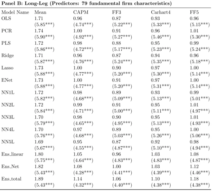
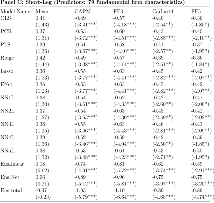
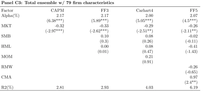
I adjust the spread portfolio returns by existing risk factor model. By regressing portfolio return on factor returns in each model, I filter out the excess return explained by these risk factors and retain the regression intercepts as our estimate of risk-adjusted returns (alpha). Risk-adjustment is done for spread portfolio, long-leg portfolio, and short-leg portfolio. Table 5 to Table 7 reports tne alphas (%) over the full sample period: 1978:01-2017:12 for the three sets of predictors respectively.
Table 5 reports the results for lagged return. Raw excess returns are adjusted by
four factor models: CAPM, Fama and French(Fama, French (1993)) three-factor model, Carhart (Carhart (1997)) four-factor model, and Fama and French (Fama, French (2015)) five-factor model. Newey-West t-statistics with 12 lags are reported in parentheses. First, risk-adjustment does not weaken either statistical or economical significance of our portfolio alpha. The most surprising result is that our results remain unaffected by Carhart 4 fac-tors, which includes a momentum factor. This could be because our model includes month t-1 to month t-120 historical return as predictors while the momentum factor in Carhart model is based on prior return from month t-2 to month t-12. Second, I further decompose spread portfolio into long- and short-leg and reports the results in Panel B and Panel C. De-composition shows stark contrast between long-leg and short-leg portfolio returns. Long-leg return is almost cut by half while short-leg return is actually enhanced (more negative and statistically significant) after risk-adjustment. This suggests that our long-leg portfolio does a mediocre (but still statistically significant) job at identifying winner stocks than common
risk factors 29, while our short-leg portfolio is doing exceptionally better. Third, network
models outperform linear models for both long- and short-leg. Take FF5-adjusted return
29For ensemble portfolios, at least 50% of raw excess return comes from their exposure to FF-5 factors. For individual models, common risk factors explain 60% to 70% of raw excess returns.
Fig. 4. Portfolio Returns (%) and Cumulative Portfolio Value 1978:01-2017:12 (Predictors: Lagged Returns)
120 lagged returns are used for predictors. Panel (A) reports the monthly spread portfolio return over the time period from 1978:01 to 2017:12. To enhance visualization, I smooth the monthly return with 12-month moving average values. Panel (B) reports the cumulative portfolio value over the time period from 1978:01 to 2017:12 after initial investment of one dollar. At the beginning of each month, I independently sort stocks into quintile portfolios on predicted returns from each model and construct spread portfolios by buying the best-predicted portfolio and selling the worst-best-predicted portfolio. For a given family of models, ensemble portfolios are constructed by buying the winner quintile agreed-upon unanimously by all models in the family and selling the unanimous loser quintile. Linear family includes OLS, PCR, PLS, Ridge, Lasso, and Elastic net. Network family includes 5 neural networks. Total ensemble includes both linear and network families, totalling 11 models.
Fig. 5. Portfolio Returns (%) and Cumulative Portfolio Value 1978:01-2017:12 (Predictors: Moving Average Signals)
60 price and 60 trading volume moving average signals are used for predictors. Panel (A) reports the monthly spread portfolio return over the time period from 1978:01 to 2017:12. To enhance visualization, I smooth the monthly return with 12-month moving average values. Panel (B) reports the cumulative portfolio value over the time period from 1978:01 to 2017:12 after initial investment of one dollar. At the beginning of each month, I independently sort stocks into quintiles portfolios on predicted returns from each model and construct spread portfolios by buying the best-predicted portfolio and selling the worst-predicted portfolio. For a given family of models, ensemble portfolios are constructed by buying the winner quintile agreed-upon unanimously by all models in the family and selling the unanimous loser quintile. Linear family includes OLS, PCR, PLS, Ridge, Lasso, and Elastic net. Network family includes 5 neural networks. Total ensemble includes both linear and network families, totalling 11 models.
Fig. 6. Portfolio Returns (%) and Cumulative Portfolio Value 1978:01-2017:12 (Predictors: Firm Characteristics)
79 firm fundamentals are used for predictors. Panel (A) reports the monthly spread portfolio return over the time period from 1978:01 to 2017:12. To enhance visualization, I smooth the monthly return with 12-month moving average values. Panel (B) reports the cumulative portfolio value over the time period from 1978:01 to 2017:12 after initial investment of one dollar. At the beginning of each month, I independently sort stocks into quintiles portfolios on predicted returns from each model and construct spread portfolios by buying the best-predicted portfolio and selling the worst-best-predicted portfolio. For a given family of models, ensemble portfolios are constructed by buying the winner quintile agreed-upon unanimously by all models in the family and selling the unanimous loser quintile. Linear family includes OLS, PCR, PLS, Ridge, Lasso, and Elastic net. Network family includes 5 neural networks. Total ensemble includes both linear and network families, totalling 11 models.
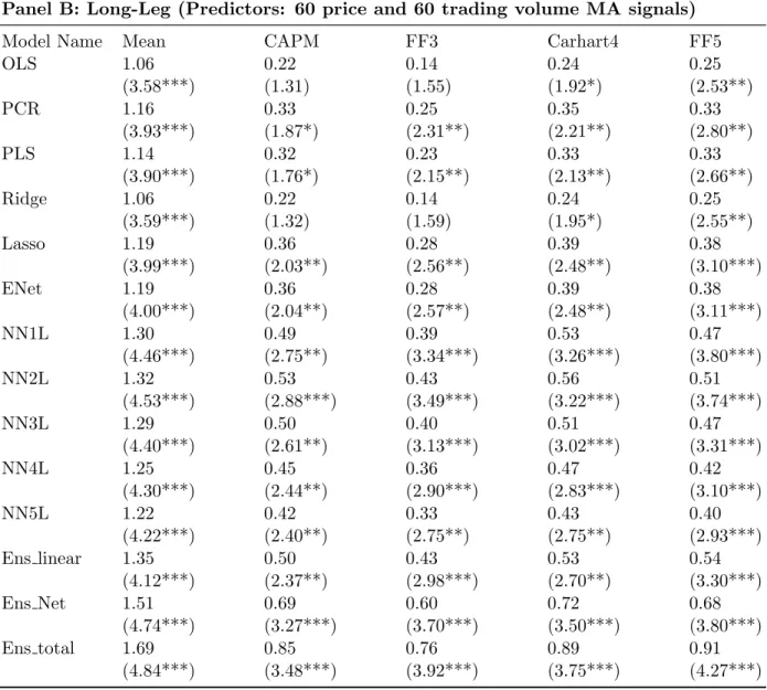
for example, for long-leg, network ensemble (linear ensemble) model generates a return of 0.73% (0.54%); for short-leg, network ensemble (linear ensemble) model generates a return of -0.90% (-0.63%).
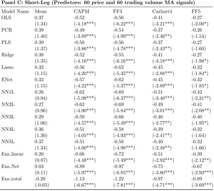
Table 6 reports the result for price and trading volume moving average signals. Results in table 6 resemble those in table 5 except for two points. First, individual models appear to be more sensitive to risk-adjustment than in lagged return setting. Statistical significance are dampened for all individual models except for NN1L and NN2L and economic significance is also reduced by a greater margin than in lagged return setting. On the other hand, the ensemble models are more robust to adjustment than individual models and their risk-adjusted returns are only slightly reduced. Second, the source of increased sensitivity comes from the short-leg. Comparing table 6 panel (C) with the same panel in table 5 shows that the short-leg of moving average signals only marginally outperforms (if at all) common risk factors and statistical significance is poor. As a result, the risk-adjusted spread returns in the moving average signal setting and the lagged return setting are pulled closer than their respective raw returns.
Table 7 reports the result for fundamental firm characteristics. The results appear one-sided. The majority of risk-adjusted return for the fundamental portfolios come from their long-leg and the short-leg contributes only a small portion. For example, the risk-adjusted returns of neural networks long-leg portfolios are approximately 1%, while the corresponding short-leg returns are only -0.4%. In addition, all of the long-leg portfolio returns remain significant at 1% level, while none of the short-leg portfolio returns are significant at 1% level.
Overall, I find that the long-leg for fundamental characteristics performs the best among all long-leg portfolios and is least affected by risk-adjustment and the short-leg for lagged return performs the best among all short-leg portfolios. I also find that the lagged return setting relies on long- and short-leg portfolios somewhat symmetrically for excess return while the other two settings rely more heavily on their long-leg rather than short-leg for excess return. This phenomenon is especially salient for fundamental variable setting, which relies on its long-leg for both economic and statistical significance, and less so for moving average signal setting, whose short-leg contributes a decent portion of economic significance. Finally, I find that most ensemble portfolios survive risk-adjustment even when their component models do not. This reinforces our point that ensemble method helps decouple the correlation of individual models with common risk factors and improves predictive power beyond those risk factors.
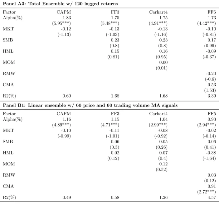
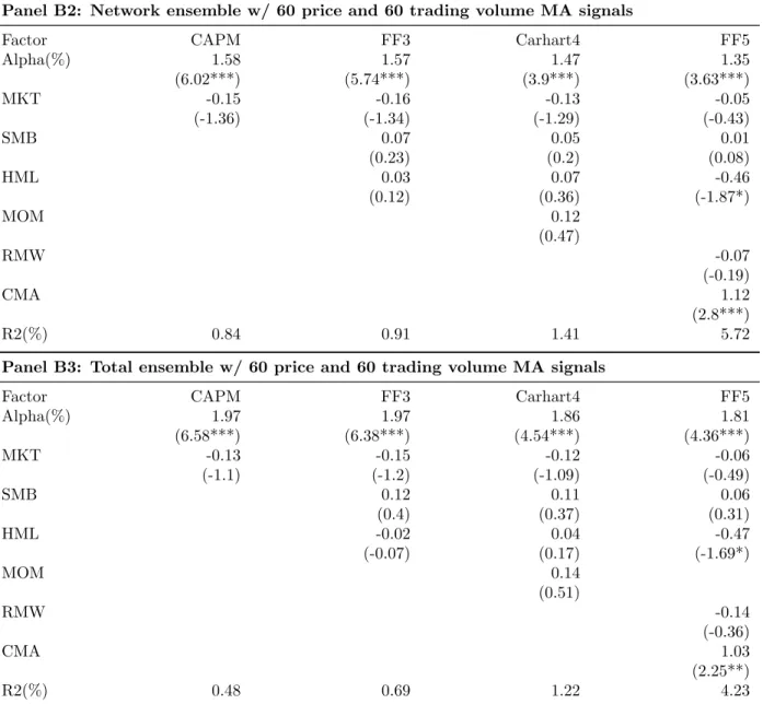
Table 8 reports the exposure to common risk factors of ensemble portfolios. Consistent with our finding in table 5 panel (A), ensemble portfolios for lagged return mostly have