A data driven binning strategy for the
construction of insurance tariff classes
Roel Henckaerts, Katrien Antonio, Maxime Clijsters and Roel Verbelen
AFI_17115
construction of insurance tariff classes
Roel Henckaerts1,3, Katrien Antonio1,2,3,4, Maxime Clijsters1 and Roel Verbelen1,3,4
1Faculty of Economics and Business, KU Leuven, Belgium.
2Faculty of Economics and Business, University of Amsterdam, The Netherlands.
3LRisk, Leuven Research Center on Insurance and Financial Risk Analysis, KU Leuven, Belgium. 4LStat, Leuven Statistics Research Center, KU Leuven, Belgium.
May 12, 2017
Abstract
We present a fully data driven strategy to incorporate continuous risk factors and geograph-ical information in an insurance tariff. A framework is developed that aligns flexibility with the practical requirements of an insurance company, its policyholders and the regulator. Our strategy is illustrated with an example from property and casualty (P&C) insurance, namely a motor insurance case study. We start by fitting generalized additive models (GAMs) to the number of reported claims and their corresponding severity. These models allow for flexible statistical modeling in the presence of different types of risk factors: categorical, continuous and spatial risk factors. The goal is to bin the continuous and spatial risk factors such that categorical risk factors result which capture the effect of the covariate on the response in an accurate way, while being easy to use in a generalized linear model (GLM). This is in line with the requirement of an insurance company to construct a practical and interpretable tariff that can be explained easily to stakeholders. We propose to bin the spatial risk factor using Fisher’s natural breaks algorithm and the continuous risk factors using evolutionary trees. GLMs are fitted to the claims data with the resulting categorical risk factors. We find that the resulting GLMs approximate the original GAMs closely, and lead to a very similar premium structure.
Key Words: P&C insurance pricing, frequency, severity, continuous risk factors, spatial risk
factor, data driven binning, generalized additive models (GAMs), Fisher’s natural breaks, evolutionary trees, generalized linear models (GLMs)
1 Introduction 2
1
Introduction
An insurance portfolio offers protection against a specified type of risk to a collection of poli-cyholders with various risk profiles. Insurance companies differentiate premiums to reflect the heterogeneity of risks in their portfolio. A flat premium across the entire portfolio would encour-age good risks to leave the company and accept a better offer elsewhere such that the insurer is left with bad risks which pay a too low premium. To avoid such lapses, insurance companies use risk factors (or: rating factors) to group policyholders with similar risk profiles in tariff classes. Premiums are equal for policyholders within the same tariff class and should reflect the inherent riskiness of each class. The process of constructing these tariff classes is also known as
risk classification, see Denuit et al. (2007); Antonio and Valdez (2012); Paefgen et al. (2013).
Pricing (or: ratemaking, tarification) through detailed risk classification is the mechanism for insurance companies to compete and to reduce the cost of insurance contracts. In a highly competitive market many rating factors are used to classify risks and to differentiate the price of an insurance product.
Property and casualty (P&C, or: non-life, general) insurance pricing typically makes use of categorical, continuous and spatial risk factors. Categorical risk factors have a discrete number of possible outcomes or levels. Examples of categorical risk factors for motor insurance are the type of coverage and type of fuel of the car. Continuous risk factors can attain all values within a specified range. Examples of continuous risk factors for motor insurance are the age of the policyholder and the horsepower of the car. A spatial risk factor contains information about the policyholder’s residency. To capture the spatial heterogeneity one can for example use the postal code of the municipality where the policyholder resides as a rating factor. In motor insurance, this serves as a proxy for the region where a policyholder drives his car.
Constructing tariff classes is rather straightforward when all risk factors are categorical; each tariff class then represents a certain combination of levels of the categorical risk factors. The continuous and spatial risk factors can be interpreted as categorical factors with many levels,
also called multi-level factors by Ohlsson and Johansson(2010). It is however inefficient to take
all these levels into account separately since this will result in too many tariff classes with very few policyholders. A better approach is to transform the continuous and spatial risk factors
with many levels in categorical risk factors with fewer levels, also called binning by Kuhn and
Johnson (2013). In this paper we present a data driven strategy to bin continuous and spatial risk factors in order to obtain categorical risk factors with a limited number of levels. After this binning procedure it is again straightforward to construct the corresponding tariff classes. Actuaries examine historical claims data to estimate the cost of offering the insurance cover, i.e. the premium, to policyholders in a specific tariff class. Insurance companies maintain large databases with policy(holder) characteristics and claim histories which enable the actuary to build risk-based pricing models. Actuarial models for P&C insurance pricing put focus on two components: a predictive model for the frequency of claims and a predictive model for the
severity of claims (see Denuit et al., 2007; Frees et al., 2014; Parodi, 2014). Claim frequency
refers to the number of claims per unit of exposure. Exposure, as described in McClenahan
(2001), can be seen as a rating unit and measures to which degree the policyholder is exposed to the insured risk. An example of exposure in an insurance product is the fraction of the year for which premium has been paid and therefore coverage is provided. Severity is the average claim cost, expressed as the ratio of the total loss to the corresponding number of claims causing this total loss, over a specific period of insurance.
Frequency and severity are typically assumed to be independent and the resulting pure premiun (or: risk premium) is the product of the expected value of the frequency and the expected
value of the severity (see Klugman et al.,2012). Alternatives for this independence assumption
are investigated in the literature, allowing dependence between frequencies and severities (see Gschl¨oßl and Czado, 2007; Czado et al., 2012). A risk margin taking model risk and pure randomness into account, as well as other premium elements (e.g. profit, commissions, taxes),
is added on top of the pure premium to end up with a commercial tariff (see Wuthrich,2016).
Generalized linear models (GLMs), developed by Nelder and Wedderburn (1972), have become
the industry standard to develop predictive models for frequency and severity (see Haberman
and Renshaw, 1997; Denuit et al.,2007; De Jong and Heller, 2008; Frees, 2015). GLMs allow the response variable to follow any distribution in the exponential family. The Poisson distri-bution is particularly interesting for claim frequency models whereas the gamma and lognormal distributions are often used for claim severity modeling. Covariates enter a GLM through a linear predictor, leading to interpretable effects of the risk factors on the response. Such a linear predictor is however less suited for continuous risk factors that relate to the response in a non-linear way, since transformations of the covariate are needed to capture a non-linear
effect. Generalized additive models (GAMs), developed by Hastie and Tibshirani (1990),
ex-tend the framework of GLMs and allow for smooth continuous effects in the predictor structure. This results in a statistically more flexible model compared to the GLM. In practice however, actuaries tend to prefer the simplicity of GLMs with categorical risk factors over GAMs with smooth effects, because pricing models should be interpretable, intuitive, explainable to clients and regulators, easy to program and adjustable to marketing needs and benchmark studies with competitors. Therefore our contribution designs a strategy to construct tariff classes in GLMs in a data driven way.
This paper should be framed in between two existing approaches to handle different types of risk factors in the literature on insurance pricing. One strand of literature uses predefined bins for
the continuous and spatial risk factors (seeFrees and Valdez,2008;Antonio et al.,2010). These
bins, which are constructed without much motivation, are then used in GLMs. Dougherty et al.
(1995)gives an overview of methods to bin variables to be used in a (generalized) linear model, but a disadvantage of those methods is that the response variable is not taken into account in the binning process. Another strand of literature develops GAMs for pricing with flexible effects
of continuous and spatial risk factors (see Denuit and Lang, 2004; Klein et al., 2014). What is
lacking is a general framework that aligns the statistical advantages of flexible modeling with GAMs to the requirements of a production environment in an insurance company. This paper tries to fill this gap by starting from GAMs with smooth effects and transforming these models into GLMs with categorical effects that satisfy the practical needs of an insurance company. Our strategy bins the continuous and spatial risk factors based on their GAM effects, resulting in categorical risk factors which are easily deployed in a GLM.
This paper is structured as follows. In Section 2we present the claims data set and in Section3
we fit flexible GAMs for frequency and severity to this data set. In Section4we bin the spatial
and continuous effects using Fisher’s natural breaks and evolutionary trees. In Section 5 we fit
2 Claims data set 4
2
Claims data set
We illustrate our methodology with a motor third party liability (MTPL) insurance portfolio
from a Belgian insurer in 1997.1 Each record in the data set represents a unique policyholder
who is observed during a certain policy period, ranging from one day to one year. The risk factors are registered at the start of the policy period and remain constant during this period.
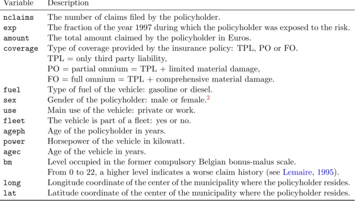
The data set contains 163 231 policyholders and the available variables are listed in Table 1.
Variable Description
nclaims The number of claims filed by the policyholder.
exp The fraction of the year 1997 during which the policyholder was exposed to the risk.
amount The total amount claimed by the policyholder in Euros.
coverage Type of coverage provided by the insurance policy: TPL, PO or FO. TPL = only third party liability,
PO = partial omnium = TPL + limited material damage, FO = full omnium = TPL + comprehensive material damage.
fuel Type of fuel of the vehicle: gasoline or diesel.
sex Gender of the policyholder: male or female.2
use Main use of the vehicle: private or work.
fleet The vehicle is part of a fleet: yes or no. ageph Age of the policyholder in years. power Horsepower of the vehicle in kilowatt.
agec Age of the vehicle in years.
bm Level occupied in the former compulsory Belgian bonus-malus scale.
From 0 to 22, a higher level indicates a worse claim history (see Lemaire,1995).
long Longitude coordinate of the center of the municipality where the policyholder resides.
lat Latitude coordinate of the center of the municipality where the policyholder resides.
Table 1: MTPL: overview of the available variables.
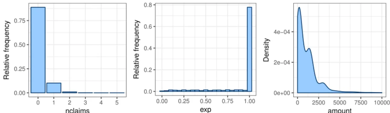
Figure 1 illustrates how nclaims, exp and amount from Table 1 are distributed in the MTPL
data set. Most policyholders (88.79%) are claim-free during their insured period. A substantial number of policyholders (10.14%) files one claim and the remaining ones (1.07%) file two, three, four or five claims. Most policyholders (77.33%) have an exposure equal to one and are therefore covered by the insurance and exposed to the risk during the entire year. The exposure of the other policyholders (22.67%) is equally spread out between zero and one. Policyholders with an exposure lower than one have surrendered the policy during the year or started the policy in the course of the year. The overall claim frequency of the portfolio, calculated as the ratio of the total number of claims and the total exposure in years, is equal to 13.93%. Claims mainly involve small amounts. The total claim amount exceeds 10 000 Euro for only 2% of the claiming policyholders. The overall claim severity of the portfolio, calculated as the ratio of the total
claim amounts and the total number of claims, is equal to 1620.06 Euro.
1A sample from this data set is analyzed inDenuit and Lang(2004);Klein et al.(2014). 2
In the Test-Achats Ruling, the Court of Justice of the EU prohibited the use of gender in insurance tariffs to avoid discrimination between males and females regarding pricing as from 21 December 2012. Notice of the European Commission: http://ec.europa.eu/justice/newsroom/gender-equality/news/121220_en.htm. Gender is therefore only investigated for use within an internal, technical tariff, but can not be used in a commercial tariff.
0.00 0.25 0.50 0.75 0 1 2 3 4 5 nclaims Relativ e frequency 0.0 0.2 0.4 0.6 0.8 0.00 0.25 0.50 0.75 1.00 exp Relativ e frequency 0e+00 2e−04 4e−04 0 2500 5000 7500 10000 amount Density
Figure 1: MTPL: relative frequency of nclaimsandexpand density estimate ofamount.
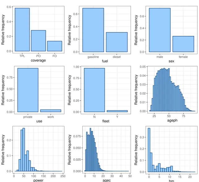
Figure 2 illustrates how the risk factors from Table 1 are distributed in the MTPL data set.
The MTPL data set contains five categorical risk factors: coverage, fuel, sex,use and fleet.
Most policyholders (58.28%) have only TPL coverage, which means that only their liability with respect to a third party (that is: another person) is covered. As in many developed countries, this coverage is compulsory in Belgium. The other policyholders have chosen for a policy which covers material damage on top of the TPL; either limited material damage in the form of a partial omnium (28.17%) or comprehensive coverage in the form of a full omnium (13.54%). Two types of fuel are used in the cars of the policyholders: gasoline (69.12%) and diesel (30.88%). Most policyholders are males (73.55%), they use their car mainly for private reasons (95.17%) and most cars are not part of a fleet (96.83%).
TheMTPLdata set contains four continuous risk factors:,ageph,power,agecandbm. Almost all
policyholders (93.53%) are aged between 25 and 75, which means that there are few young and old drivers in the insurance portfolio. Most of the cars in the insurance portfolio have less than 100 kilowatt of horsepower (97.35%) and are younger than 20 years old (99.53%). The rather low range of horsepower is nowadays outdated, but fits the less powerful cars from 1997. More than half of the policyholders reside in the two lowest bonus-malus levels (level 0: 37.77% and level 1: 16.52%). Most of the other policyholders (42.90%) have a bonus-malus level between 2 and 11 and almost no policyholders (2.81%) occupy a bonus-malus level higher than 11. It should be noted that the bonus-malus level is usually not incorporated as a risk factor in an a priori tariff. However, we keep this variable in our analysis to investigate the information contained
in this risk factor, much in line with the work of Denuit and Lang(2004);Klein et al. (2014).
The left panel of Figure 3shows a two dimensional density estimate forageph andpower. This
gives additional intuition about the distribution of the policyholders over these continuous risk
factors and shows the interplay betweenageph and power.
TheMTPL data set contains geographical information in the form of longitude and latitude
coor-dinates,longandlat, of the municipality (or: postal code area) where the policyholder resides.
The map of Belgium in Figure3visualizes the exposure in each municipality relative to the area
of the municipality. White municipalities are those where the insurer has no policyholders and is therefore not exposed to the risk of filing a claim. Municipalities in light (dark) blue represent the 20% of municipalities containing the lowest (highest) relative exposure. Few policyholders are living in the southeastern part of Belgium, the Ardennes, while a lot of policyholders are
living near some big cities of the French Community in Belgium; Brussels, Li`ege, Charleroi and
2 Claims data set 6 0.0 0.2 0.4 0.6 TPL PO FO coverage Relativ e frequency 0.0 0.2 0.4 0.6 gasoline diesel fuel Relativ e frequency 0.0 0.2 0.4 0.6 male female sex Relativ e frequency 0.00 0.25 0.50 0.75 private work use Relativ e frequency 0.00 0.25 0.50 0.75 1.00 N Y fleet Relativ e frequency 0.00 0.01 0.02 0.03 0.04 0.05 25 50 75 ageph Relativ e frequency 0.0 0.1 0.2 0 50 100 150 200 250 power Relativ e frequency 0.000 0.025 0.050 0.075 0 10 20 30 40 50 agec Relativ e frequency 0.0 0.1 0.2 0.3 0 5 10 15 20 bm Relativ e frequency
Figure 2: MTPL: relative frequency of the risk factorscoverage,fuel,sex,use, fleet,ageph,power,
agec,bm. 30 40 50 60 70 80 90 20 40 60 80 ageph po w er 2e−04 4e−04 6e−04 8e−04 Density Relative frequency low average high NA
3
Flexible models for P&C pricing using GAMs
FollowingMcClenahan(2001);Antonio and Valdez(2012)we denote withFi andSi respectively
the frequency and severity of policyholder i. Frequency is expressed as the number of claims
Ni per unit of exposure ei, while severity is expressed as the average claim amount over the
number of claims Ni. The severity Si is therefore only defined if policyholder i files a claim,
i.e. if Ni > 0. We define the pure premium πi as follows: πi = E[Fi]×E[Si], by assuming
independence between Fi and Si. In this setting we construct a predictive model for Fi using
the claim history of all policyholders in the portfolio, including those who did not file a claim,
and one for Si using the history of policyholders who filed at least one claim.
GAMs are a suitable tool for actuarial regression modeling due to their flexibility in handling different types of risk factors. These models allow for the incorporation of smooth effects of
continuous and spatial risk factors. The predictor η of the GAMs is expressed as follows:
ηi =g(µi) =β0+ p X j=1 βjxdij + q X j=1 fj(xcij) + r X j=1 fj(xsij, ysij). (1)
where µi is the mean of a response variable with a distribution from the exponential family
and g(.) is the link function. The 0/1-valued dummy variables xd represent the typical way to
code categorical risk factors in the GLM or GAM framework: a categorical risk factor with z
levels requires the choice of a reference level andz−1 dummy variables to model the differences
between the other levels and the reference level. The regression coefficientβj captures the effect
of dummy variable xdj on the predictor η. GAMs extend GLMs by including smooth functions
of continuous risk factors. Main effects are captured by the univariate smooth functions f(xc),
while interaction and spatial effects are expressed by bivariate smooth functions f(xs, ys).
GAMs form the starting point of our pricing strategy and we search for the optimal model by
using the Akaike information criterium (AIC, see Akaike,1974) and the Bayesian information
criterion (BIC, seeSchwarz,1978). Both take goodness of fit and model complexity into account
and are defined as follows:
AIC =−2·logL+ 2·EDF
BIC =−2·logL+ log(n)·EDF (2)
where logLis the log-likelihood of the model,nis the number of observations in the data set and
EDF represents the effective degrees of freedom which corresponds to the number of parameters in a GLM. Both AIC and BIC measure the goodness of fit by minus two times the log-likelihood supplemented with a complexity penalty. The BIC penalty is more severe and BIC will therefore favor less complex models. We continue our search for the optimal GAM with BIC as model
selection criterion since we want to favor well performing models that are as simple as possible.3
Note that lower AIC/BIC values indicate better models.
We fit the GAMs to the claims data on frequency and severity separately and follow - for both predictive models - a two-step strategy to select the appropriate set of risk factors to be included
in (1). The first step performs an exhaustive search for the optimal GAM without taking into
account interactions between the risk factors. In the second step, we perform an additional exhaustive search to search for meaningful interactions which improve the model fit. We only try to add interactions between continuous risk factors which have been selected in the first step. 3For illustrative purposes we use BIC to select the optimal GAM, which serves as the starting point of our strategy. In the subsequent binning steps we use AIC as selection criterion.
3 Flexible models for P&C pricing using GAMs 8
We use R and the mgcv package developed by Wood (2006) to fit the GAMs. The smooth
functions f from (1) are represented by penalized thin plate regression splines, wich are low
rank approximations of the thin plate splines of Duchon (1977). For details on thin plate
(regression) splines we refer to Section 2 of Wood(2003)and Section 4.1.5 of Wood(2006). We
construct the interaction effects as tensor product interactions which exclude the main effects
of the continuous risk factors, see Section 4.1.8 of Wood (2006) for details on tensor product
smooths. We define the interactions in such a way that we can interpret them as corrections on top of the main effects which are included separately in the model. The model parameters are estimated by maximizing the penalized log-likelihood via penalized iteratively reweighted
least squares (P-IRLS), see Section 4.3 of Wood (2006) for details on this procedure. The
smoothness of the splines is controlled by a smoothing parameter, which will make a trade-off between penalizing a bad fit to the data and penalizing the ‘wiggliness’ of the spline. Smoothing
parameters are estimated via Generalized Cross Validation (GCV, seeCraven and Wahba,1978)
or via an Un-Biased Risk Estimator (UBRE, seeWahba,1990) when the scale parameter in the
distribution of the response is unknown or when it is known, see Section 4.5.4 ofWood (2006).
3.1 Frequency
In this section we focus on developing a flexible regression model for claim frequencies. We
assume a Poisson distribution for nclaimsand demonstrate our approach within this
distribu-tional setting. This is a common assumption in the insurance pricing industry and is in line
with earlier work on this data set (seeDenuit et al.,2007). An actuary can however easily apply
our approach to other distributional settings (e.g. negative binomial).
The goal is to explain the number of claims nclaims reported by a policyholder, for given
exposure exp, using different types of risk factors. Our starting point is a Poisson GAM which
includes all categorical risk factors coverage, fuel, sex, use and fleet together with main
effects of all continuous risk factors ageph, power, agec and bm and a spatial effect based on
longandlat. This GAM, which is not yet using any interaction terms, is formulated as follows:
log(E(nclaims)) = log(exp) +β0+β1coverageP O+β2coverageF O+β3fueldiesel+
β4sexf emale+β5usework+β6fleetY +f1(ageph) +f2(power)+
f3(agec) +f4(bm) +f5(long,lat).
(3)
The logarithm of exposure is included in the model as an offset, such that the expected number
of claims is proportional to the exposure. The five categorical risk factors are coded with
dummy variables by taking the level with the largest amount of exposure as reference level: coverageT P L,fuelgasoline,sexmale,useprivateand fleetN. The functionsf1,f2,f3 and f4 are
univariate smooth effects of continuous risk factors. The spatial effect, f5, is a bivariate smooth
function of the latitude and longitude coordinates.
We perform an exhaustive search over all possible combinations of explanatory variables in
order to find the best GAM fit. The full model in (3) contains 10 risk factors: 5 categorical, 4
continuous and 1 spatial. All 1024 different models that can be formed by including or excluding
these 10 risk factors are evaluated.4 The model with the lowest BIC value of all 1024 investigated
models is given by:
log(E(nclaims)) = log(exp) +β0+β1coverageP O+β2coverageF O+β3fueldiesel+
f1(ageph) +f2(power) +f3(bm) +f4(long,lat).
(4) 4
Two categorical risk factors, coverage and fuel, three continuous risk factors, ageph, power and bm, and the spatial risk factor are included in the optimal specification for the predictor.
We now investigate whether the model in (4) can further be improved by adding interaction
effects between the continuous risk factors. Such interaction effects are not considered in the
studies of Denuit and Lang (2004); Klein et al. (2014). For demonstration purposes we only
include interaction effects among continuous risk factors and not among categorical risk factors or between a continuous and a categorical risk factor. An interaction effect between a continuous and categorical risk factor will give rise to a smooth effect of the continuous risk factor for every level of the categorical risk factor. Adding these types of interactions will therefore only result in a more complex model without contributing added value to the demonstration of our strategy for the construction of tariff classes.
We examine interactions between the continuous risk factors already included in (4). The only
possible interactions betweenageph,powerandbmare: ageph-power,ageph-bmandpower-bm.
Incorporating the interaction ageph-power results in a decrease of BIC whereas adding the
other two interaction effects always results in an increase of BIC. The interactionageph-power
is therefore added to the model in (4) and our resulting GAM for claim frequency is given by:
log(E(nclaims)) = log(exp) +β0+β1coverageP O+β2coverageF O+β3fueldiesel+
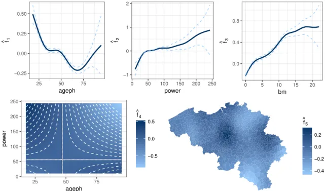
f1(ageph) +f2(power) +f3(bm) +f4(ageph,power) +f5(long,lat).
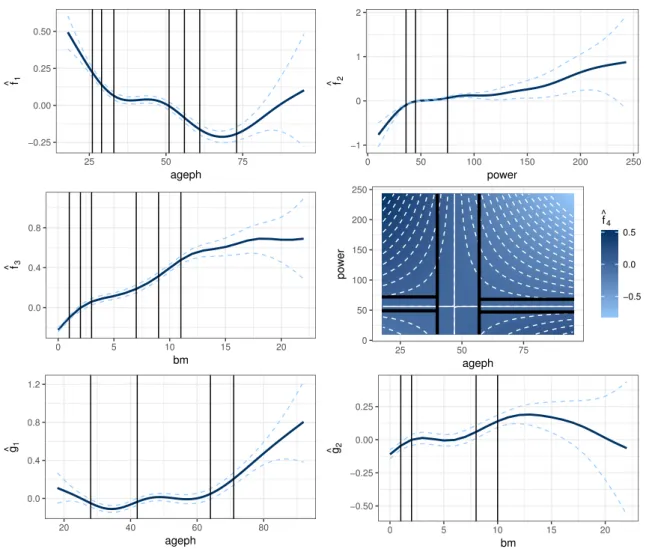
(5) −0.25 0.00 0.25 0.50 25 50 75 ageph f ^ 1 −1 0 1 2 0 50 100 150 200 250 power f ^ 2 0.0 0.4 0.8 0 5 10 15 20 bm f ^ 3 0 50 100 150 200 250 25 50 75 ageph po w er −0.5 0.0 0.5 f ^ 4 −0.4 −0.2 0.0 0.2 f ^ 5
Figure 4: MTPL-frequency: fitted smooth GAM effects from (5). Top row: main effects ˆf1(ageph),
ˆ
f2(power) and ˆf3(bm). Bottom row: interaction effect ˆf4(ageph,power) and spatial effect
ˆ
3 Flexible models for P&C pricing using GAMs 10
Figure4displays the five fitted smooth functions: ˆf1(ageph), ˆf2(power), ˆf3(bm), ˆf4(ageph,power)
and ˆf5(long,lat) from (5). The top row shows the fitted smooth effects of the risk factorsageph,
power and bmin solid lines. The dashed lines represent the 95% pointwise confidence intervals, which are wider in regions with scarce data. Young policyholders appear to be risky drivers, which might be explained by their driving style or lack of experience behind the wheel. This riskiness decreases over increasing ages and stabilizes around the age of 35. It increases slightly between ages 45 and 50, possibly due to the fact that children of policyholders in their late 40s - early 50s start to drive with their parents’ car. After age 50 the riskiness decreases again until the age of 70, after which it starts increasing again. This implies that seniors report more car accidents when growing older. Note however the widening confidence interval for these high ages
due to the rarity of old policyholders in our portfolio. The smooth effect of powershows a steep
increase over the interval from 0 to 50 kilowatt and a more gradual increase from 50 kilowatt onwards. This implies that policyholders driving a more powerful vehicle are more likely to
report a claim. The smooth effect of bm shows a steady increase over increasing bonus-malus
levels. This effect is in line with our intuition, since policyholders occupying high bonus-malus levels have worse claim histories compared to policyholders with low bonus-malus levels.
The fitted interaction effect between ageph and power is displayed in the bottom left panel of
Figure 4. A negative (positive) correction, coloured in light blue (dark blue), indicates that the
combined main effects of ageph and power overestimate (underestimate) the annual expected
claim frequency. The combinations low ageph - low power and high ageph - high power are
therefore less risky than the two main effects predict. The combinations highageph- low power
and lowageph - highpower are therefore more risky than the two main effects predict. Among
others, the results of our preferred GAM show that young policyholders driving a more powerful car imply a high risk for the insurer, at least in terms of the claim frequency.
The fitted spatial effect is displayed in the bottom right panel of Figure 4. Note that this
map does not indicate how likely claims are to occur in each municipality, but it reflects in which municipalities the more risky policyholders reside. Although a policyholder can have an accident in any municipality, we can assume that he will drive quite often in his own municipality. Moreover, the municipality serves as a proxy for socio-economic characteristics that characterize the neighborhood where the policyholder resides. The municipalities are colour coded where light blue (dark blue) indicates a municipality where policyholders reside which have, on average, few (many) car accidents. The region around Brussels, in the center of Belgium, is associated with the highest accident risk. Traffic is very dense in this area, which is reflected in a higher expected annual claim frequency for policyholders who live here. The southeastern, northeastern and western parts of Belgium are less densely populated, which is reflected in a lower expected annual claim frequency for policyholders who live here.
3.2 Severity
We now focus on developing a flexible regression model for claim severities. Our data set does not contain individual claim amounts, but we have the total claim amount and the number of
claims at our disposal. We therefore work with the average cost of a claim where avgis defined
as the ratio of amountand nclaims. We use nclaims as a weight in our regression model and
assume a lognormal distribution for avg. This is a common assumption in the insurance pricing
industry and is in line with earlier work on this data set (see Denuit and Lang, 2004). An
We follow the fitting procedure outlined in Section3.1and start with finding an optimal lognor-mal GAM without interation effects. In a next step we look for interactions between continuous risk factors that improve the model fit. In the severity fitting procedure we can only use
obser-vations of policyholders who actually filed a claim, i.e. nclaims>0, which accounts for 18 295
records in our MTPL data set. The very large claims are excluded from our analysis since these
are not the focus when developing a tariff structure. Using techniques from Extreme Value
Theory (EVT) Denuit and Lang (2004); Klein et al. (2014) obtain a threshold of 81 000 Euro
which separates small, attritional losses from large losses. For 19 records the average claim cost exceeds this threshold. We therefore obtain 18 276 records below the threshold to fit our severity model.
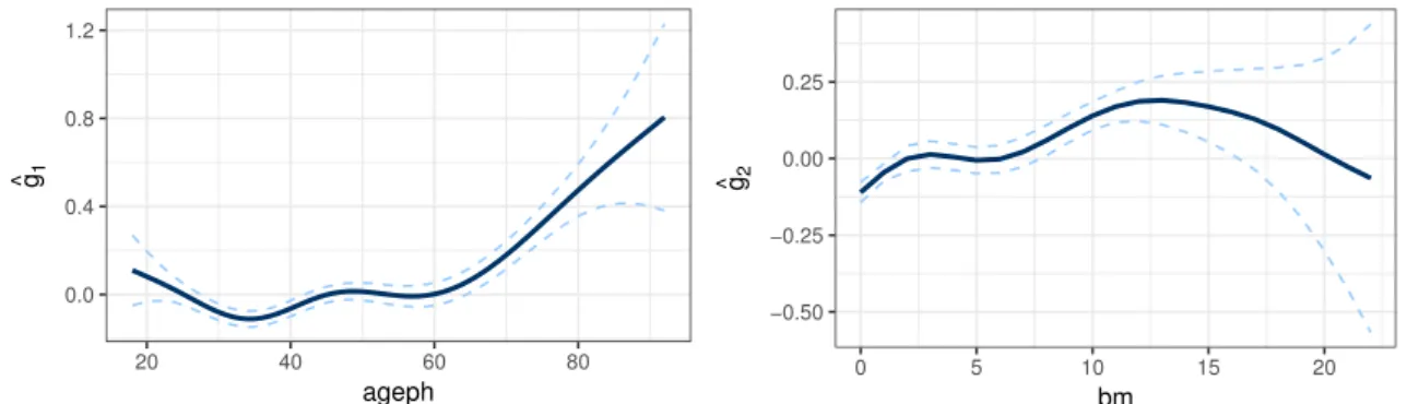
Our preferred model for claim severity is the lognormal GAM given by:
E(log(avg)) =γ0+γ1coverageP O+γ2coverageF O+g1(ageph) +g2(bm). (6)
A Gaussian distribution is assumed for the response log(avg), such that the average amount of
a claim follows a lognormal distribution. Only one categorical risk factor, coverage, and two
continuous risk factors, ageph and bm, are selected. We find no relevant interaction or spatial
effect for severity. As documented in actuarial pricing literature (see Charpentier and Boucher,
2014), severity models tend to have fewer relevant risk factors compared to frequency models.
Claim severity is more difficult to explain by risk factors than claim frequency for at least two reasons. First of all, one has less data available to fit a severity model. Secondly, the driver has almost no control over the cost of an accident.
Figure 5 displays the two fitted smooth functions: ˆg1(ageph) and ˆg2(bm) from (6). Going from
ages 18 to 35, we can observe a decrease of the average claim cost. This indicates that very young drivers are involved in more severe car accidents. The average claim cost starts to increase again for policyholders older than 35, stabilizes in the age interval 45 to 60 after which it starts to increase again. A possible explanation might be the fact that older policyholders drive more expensive cars and repairing costs increase. The age of the policyholder might be operating as a proxy for the price of the car. Unfortunately we do not have that information in our data set to confirm this. The average claim cost increases with increasing bonus malus levels. There is however a stabilizing region around level 5 and the average claim cost decreases from bonus malus level 13 onwards. Because of the scarceness of data for the high bonus malus levels one can not conclude much about this region, as the widening confidence bounds illustrate.
0.0 0.4 0.8 1.2 20 40 60 80 ageph g^1 −0.50 −0.25 0.00 0.25 0 5 10 15 20 bm g^2
4 Data driven binning methods for the smooth GAM effects 12
4
Data driven binning methods for the smooth GAM effects
The GAM model formulas (5) and (6) are optimal, according to BIC, for claim frequency and
severity in the MTPL data set. These models offer a high degree of flexibility for the spatial and
continuous risk factors, which is very appealing from a statistical modeling point of view. For
practical purposes, as discussed in Section 1, insurers prefer a pricing model where each risk
factor is categorical. This makes the price list easy to implement, explain and adjust. In this section we present a data driven approach to bin the spatial and continuous risk factors of the
predictors (5) and (6). In Section4.1we bin the spatial risk factor, which is only present in the
frequency model. In Section 4.2 we bin the continuous risk factors, which are present in both
the frequency and severity models. Once all risk factors are categorical, it is straightforward to
estimate a GLM with the risk factors coded by dummy variables (see Section 5).
4.1 Spatial effect
We first put focus on binning the fitted continuous spatial effect ˆf5(long,lat) from the frequency
model (5). For each of the 1146 Belgian municipalities we have a single number which represents
the spatial riskiness of that municipality: si = ˆf5(longi,lati) for i ∈ {1, ...,1146}. The goal
therefore is to group the municipalities with similar spatial riskiness together. We use the
classIntpackage inR, developed byBivand(2015), to compare four different binning methods: • Equal intervals. The range of the spatial effect ˆf5(long,lat) is divided in k bins of
equal length: max(si)−kmin(si), where the maximum and minimum are taken over alli. This
approach can give good results for uniformly distributed data, but tends to perform poorly for skewed data.
• Quantile binning. Each bin will contain approximately 1146k municipalities where k equals the number of bins. This method is often the default in statistical software packages, though it can give very misleading results. Similar observations can be assigned to different bins in order to make sure that each bin contains the same number of observations.
• Complete linkage. This method performs agglomerative hierarchical clustering (see
Kaufman and Rousseeuw, 1990). Initially each municipality forms its own bin and in
every iteration the two bins closest to each other are merged. The distance between binsi
and j is equal to the distance between their most distant points: d(i, j) = max|su(i)−s(vj)|
∀u, v :s(ui) ∈ i, sv(j) ∈ j, where u and v run over all possible combinations of points from
bin iand binj. Bins with remote observations will only be merged in a late stage of the
iteration process.
• Fisher’s natural breaks. This iterative algorithm, developed by Fisher (1958) and
discussed inSlocum et al.(2005), maximizes the homogeneity within bins. Bins are created
such that every observation s(ui) in bin i is as close as possible to the average of its bin
¯
s(i). This is done by minimizing the sum of squared distances between observations s(i)
u
and the respective bin means ¯s(i): Pk
i=1
Pni u=1(s
(i)
u −s¯(i))2. Here,iruns over the different
bins, u runs over the municipalities within each bin, k is the number of bins and ni the
We compare the results of the different binning methods using two measures: the goodness of variance fit (GVF) and the tabular accuracy index (TAI). The GVF and TAI are defined as
follows by Armstrong et al.(2003):
GVF = 1− Pk i=1 Pni u=1(s (i) u −s¯(i))2 P1146 u=1(su−¯s)2 (7) TAI = 1− Pk i=1 Pni u=1|s (i) u −¯s(i)| P1146 u=1 |su−s¯| (8)
where k and ni indicate the number of bins and the number of municipalities in bin i. The
denominator in (7) and (8) measures the deviation of each municipality from the global average.
The numerator in (7) and (8) measures the deviation of each municipality from its bin average.
For both measures a value closer to 1 indicates small variance within the bins compared to the global variance and hence a more homogeneous binning of the municipalities.
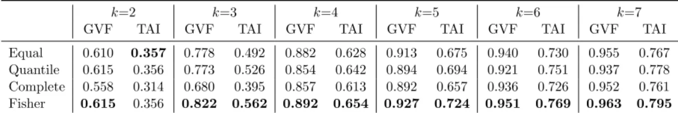
Table 2 compares the performance of the four binning methods for different number of bins k.
We denote the highest values for the GVF and TAI in bold in every column where we use the fourth digit behind the decimal point in case of a tie in the presented values. Fisher’s natural breaks algorithm outperforms the other methods in eleven out of twelve cases. This method clearly results in the most homogeneous binning and is therefore the preferred method to bin
the spatial effect ˆf5(long,lat) from the frequency model (5). The equal intervals method is
performing rather well despite its simplicity; it attains the second best GVF in five out of six cases. Quantile binning also performs well, attaining the second best TAI in five out of six cases. The complete linkage method attains the lowest GVF/TAI in nine out of twelve cases.
k=2 k=3 k=4 k=5 k=6 k=7
GVF TAI GVF TAI GVF TAI GVF TAI GVF TAI GVF TAI Equal 0.610 0.357 0.778 0.492 0.882 0.628 0.913 0.675 0.940 0.730 0.955 0.767 Quantile 0.615 0.356 0.773 0.526 0.854 0.642 0.894 0.694 0.921 0.751 0.937 0.778 Complete 0.558 0.314 0.680 0.395 0.857 0.613 0.892 0.657 0.936 0.726 0.952 0.761 Fisher 0.615 0.356 0.822 0.562 0.892 0.654 0.927 0.724 0.951 0.769 0.963 0.795
Table 2: MTPL: the GVF and TAI for the four methods and different values forkto bin the spatial effect ˆ
f5(long,lat).
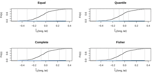
In order to get a better understanding of the resulting bins for different methods we show two
visual comparisons withk= 5. Figure6shows the empirical cumulative distribution function of
the spatial effect ˆf5(long,lat) in combination with the bins produced by the different methods.
Figure7visualizes the different spatial binning results on the map of Belgium. The four methods
result in very different bins for the spatial effect and therefore give rise to very different groupings of the municipalities. The method of equal intervals clearly divides the range of the spatial effect in five equally sized bins. A lot of municipalities are therefore grouped in the middle bin (499) whereas few municipalities are grouped in the first and last bin (39 and 111). Quantile binning produces very wide bins in the extreme ends of the support where data are scarce. Every bin contains approximately 230 municipalities. Complete linkage groups a lot of municipalities in the second bin (465) and few municipalities in the first and last bin (39 and 55). Fisher’s natural breaks algorithm results in the most homogeneous binning and seems to act as a middle ground between equal intervals and quantile binning. We obtain 300 municipalities in the middle bin and respectively 86 and 176 in the first and last bin.
4 Data driven binning methods for the smooth GAM effects 14 −0.4 −0.2 0.0 0.2 0.4 0.0 0.6 Equal f ^5(long, lat) Fn(x) −0.4 −0.2 0.0 0.2 0.4 0.0 0.6 Quantile f ^5(long, lat) Fn(x) −0.4 −0.2 0.0 0.2 0.4 0.0 0.6 Complete f ^ 5(long, lat) Fn(x) −0.4 −0.2 0.0 0.2 0.4 0.0 0.6 Fisher f ^ 5(long, lat) Fn(x)
Figure 6: MTPL: the empirical cumulative density function of the fitted spatial effect ˆf5(long,lat) in
combination with the five bins produced by the four different binning methods.
Equal [−0.48,−0.32) [−0.32,−0.15) [−0.15,0.012) [0.012,0.18) [0.18,0.34] Quantile [−0.48,−0.18) [−0.18,−0.092) [−0.092,−0.019) [−0.019,0.067) [0.067,0.34] Complete [−0.48,−0.32) [−0.32,−0.079) [−0.079,0.047) [0.047,0.23) [0.23,0.34] Fisher [−0.48,−0.27) [−0.27,−0.14) [−0.14,−0.036) [−0.036,0.11) [0.11,0.34]
Figure 7: MTPL: maps of Belgium with the municipalities grouped into five distinct bins based on the intervals produced by the four different binning methods for the spatial effect ˆf5(long,lat).
From inspecting Table 2 it follows that increasing the number of bins k results in a monotonic
increase of both the GVF and TAI. These measures can therefore not be used to choose the
number of binsksince more bins will always result in a more homogeneous binning. As motivated
in Section1, pricing actuaries ultimately prefer a GLM where all types of risk factors are coded
as categorical variables. We therefore propose to tune the optimal number of bins for the spatial effect based on the binned spatial effect which will be used in a GLM. We tune the number of
bins by considering a set of possible values for the number of spatial bins, e.g.k∈ {2,3,4,5,6,7}.
Procedure: Find the optimal number of bins for the spatial effect
Step 1 Apply Fisher’s natural breaks algorithm to calculate the bin intervals for the spatial effect, ˆf5(long,lat) from (5), where the number of bins is chosen equal to the current
value of the predefined set of values. These bin intervals are used to transform the continuous spatial effect into a categorical spatial effect.
Step 2 Estimate a new GAM where we use a predictor structure similar to (9). This GAM contains the spatial effect in a categorical format, but still uses flexible effects to model the continuous risk factors.
Step 3 Calculate AIC of the GAM with a binned spatial effect.
Table 3: Procedure to find the optimal number of bins for the spatial effect.
After applying this procedure we choose the number of bins for the spatial effect that results in the lowest AIC for the GAM with a binned spatial effect. Our approach requires the estimation of a GAM with binned spatial effect for each value in the considered set, but this extra effort
allows us to find the best fitting GLM in the end. The results in Table4illustrate that choosing
five bins results in the lowest AIC for the GAM with a binned spatial effect. We also report the BIC values of the GAMs with a binned spatial effect and conclude that choosing BIC as evaluation measure also results in five bins for binning the spatial effect.
# bins AIC BIC
2 124778.9 125047.6 3 124753.1 125023.9 4 124652.3 124928.4 5 124621.3 124907.2 6 124627.7 124921.6 7 124639.1 124942.9
Table 4: MTPL: AIC and BIC for the fitted GAM with binned spatial effect, as obtained via Fisher’s natural breaks, evaluated over a predefined set for the number of bins.
From this section we conclude that it is optimal to bin the spatial effect ˆf5(long,lat) from the
frequency model (5) with Fisher’s natural breaks algorithm in five bins. This results in the most
homogeneous binning for the spatial effect and the lowest AIC value for the GAM with a binned spatial effect. For the frequency model we continue our study with a GAM which specifies the
spatial effect as a categorical risk factor (geo). The bin [−0.036,0.11) is chosen as the reference
class since it contains the highest amount of exposure, namely 354 municipalities. This gives the following GAM specification for the frequency model:
log(E(nclaims)) = log(exp) +β0+β1coverageP O+β2coverageF O+β3fueldiesel+
β4geo[−0.48,−0.27)+β5geo[−0.27,−0.14)+β6geo[−0.14,−0.036)+β7geo[0.11,0.34]+
f1(ageph) +f2(power) +f3(bm) +f4(ageph,power).
4 Data driven binning methods for the smooth GAM effects 16
4.2 Continuous risk factors
We now put focus on binning the main and interaction effects of the continuous risk factors: ˆ
f1(ageph), ˆf2(power), ˆf3(bm), ˆf4(ageph,power) from the frequency model (9) and ˆg1(ageph),
ˆ
g2(bm) from the severity model (6).
We want to create bins where consecutive values of a continuous risk factor are grouped to-gether. The approach followed for binning the spatial effect is therefore no longer appropriate, since it might create bins where - for example - policyholders younger than 30 are grouped with policyholders older than 80. We propose the use of regression trees as a technique to perform the binning since these models produce intuitive splits in line with our requirement of grouping con-secutive values of the continuous variables, e.g. ages. In particular, we choose to use evolutionary
trees from theRpackageevtreedeveloped byGrubinger et al.(2014). These evolutionary trees
combine the framework of regression trees with genetic algorithms. Classic regression tree
meth-ods, as discussed in Breiman et al.(1984), are recursive partitioning methods that fit a model
in a forward stepwise search. Splits are chosen to maximize the homogeneity of the partitions at every step and these consecutive splits are kept fixed in all the following steps. This forward stepwise search is an efficient heuristic, but the resulting binning is only locally optimal. Evolu-tionary trees allow us to adapt earlier splits in a later stage of the fitting procedure. Thanks to
this extra flexibility, evolutionary trees are capable of finding a global optimum (see Grubinger
et al.,2014). We refer toBreiman et al. (1984);Hastie and Tibshirani (1990);Grubinger et al. (2014); for details and terminology regarding tree based predictive models.
The data that serves as input to the evolutionary trees are the main and interaction effects
from the GAMs in (9) and (6): (ageph, ˆf1), (power, ˆf2), (bm, ˆf3), (ageph, power, ˆf4), (ageph,ˆg1),
(bm,ˆg2). Hence we grow a regression tree for each of the fitted flexible effects, with the flexible
effect (e.g. ˆf1(ageph)) as response and the corresponding risk factor (e.g. ageph) as covariate.
This results in a binned version of the flexible effect which takes into account the ordering of the levels of the continuous risk factors. It is important to take the composition of the insurance portfolio into account when deciding where to split or bin the risk factors. For policyholders
older than 75, for example, the fitted smooth effect ˆf1(ageph) in Figure4is strongly increasing,
but Figure 2indicates that the portfolio does not contain many policyholders aged over 75. It is
not desirable to obtain many splits in this region, since it will only affect a small portion of the portfolio. Therefore the distribution of the policyholders with respect to a specific risk factor is
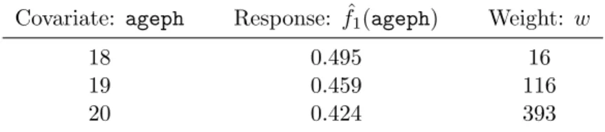
taken into account by using the number of policyholders as weights. Table5 shows a snippet of
input data for the ˆf1(ageph) tree. For example, the MTPL portfolio contains 393 policyholders
aged 20. The smooth effect for ageph= 20, ˆf1(20), therefore obtains an integer weight of 393.
The evolutionary tree will interpret this weight as if the observation pair (ageph= 20,fˆ1(20))
occurs 393 times in its input data. A constraint is imposed to make sure that bins are not too sparsely populated: each bin should at least contain 5% of the policyholders in the entire portfolio. Modifying this constraint gives insurers flexibility over the granularity of the bins.
Covariate: ageph Response: ˆf1(ageph) Weight: w
18 0.495 16
19 0.459 116
20 0.424 393
The evaluation function to measure the performance of a tree has the following form:
n·log(MSE) + 4·α·(m+ 1)·log(n) (10)
wherenis the number of observations in the input data,mis the number of leaf nodes in a tree
and α is a tuning parameter (see Grubinger et al.,2014). Note that n is equal to the sum of
all the weights since a tree interprets a weight as being the number of times that the respective
(response, covariate) pair occurs in the input data. The first term in evaluation function (10)
measures the accuracy of the tree by means of the mean squared error (MSE). For ˆf1(ageph)
-for example - this MSE looks as follows:
MSE =
Pmax(ageph)
i=min(ageph)wagephi( ˆf1(agephi)−fˆ b
1(agephi))2
Pmax(ageph)
i=min(ageph)wagephi
(11)
withwagephi the number of policyholders withageph=i, ˆf1(agephi) the fitted GAM effect for a
policyholder with ageph=iand ˆf1b(agephi) the fitted value obtained from the regression tree.
This last value is obtained as the mean of ˆf1(agephi) over all policyholders in the age bin where
ageph = i belongs to. The second term of evaluation function (10) represents a complexity
penalty in terms of the size of the tree, measured by the number of leaf nodesm, where each leaf
node corresponds to a bin. The tuning parameterαtakes care of the trade-off between accuracy
and complexity.
The evaluation function in (10) scales in a comparable manner over the four trees that bin the
frequency effects ˆf1(ageph), ˆf2(power), ˆf3(bm), ˆf4(ageph,power) because of two reasons. Firstly,
n= 163 231 for all four trees since this is the total number of policyholders in theMTPLdata set.
Secondly, the MSEs are on the same level since they deal with the variance of the effects at the level of the predictor of the frequency model. This motivates the use of a single tuning parameter αf req to construct the trees. Likewise we define αsev as the single tuning parameter for both
trees that bin the severity effects ˆg1(ageph), ˆg2(bm). For both these trees n = 18 276 and the
MSEs are again at the same level, that is the level of the predictor of the severity model. This
implies that we have two tuning parameters which can be optimized independently: αf req and
αsev. Tuning these α’s follows the same approach as tuning the number of bins for the spatial
effect in Section 4.1. We consider a set of possible values for both αf req and αsev and search
for the optimal ones. After some initial exploration, we choose to use the unequally spaced set
{1,1.5,2,. . .,9.5,10,15,20,. . .,95,100,150,200,. . .,950} for both αf req and αsev. These values allow
us to find the right balance between too complex trees (low α’s) and too simplistic trees (high
α’s). For each value in this set the procedure listed in Table6 is applied.
Procedure: Find the optimal tuning parametersαf req andαsev for the evolutionary trees
Step 1 Fit evolutionary trees to the main and interaction effects of the continuous risk factors, (ageph, ˆf1(ageph)) et cetera, where α is chosen equal to the current value of the
predefined set of values. The splits produced by these trees are used to transform the continuous effects into categorical effects.
Step 2 Estimate a frequency and severity GLM with the resulting categorical risk factors. Step 3 Calculate AIC of the frequency GLM and the severity GLM.
Table 6: Procedure to find the optimal tuning parametersαf reqandαsevto bin the main and interaction
4 Data driven binning methods for the smooth GAM effects 18
After applying this procedure we choose the values of αf req and αsev that result in the lowest
AIC for respectively the frequency and severity GLM. Figure8shows the splits produced by the
preferred evolutionary trees with αf req = 550 andαsev = 70.
−0.25 0.00 0.25 0.50 25 50 75 ageph f ^ 1 −1 0 1 2 0 50 100 150 200 250 power f ^ 2 0.0 0.4 0.8 0 5 10 15 20 bm f ^ 3 0 50 100 150 200 250 25 50 75 ageph po w er −0.5 0.0 0.5 f ^ 4 0.0 0.4 0.8 1.2 20 40 60 80 ageph g^1 −0.50 −0.25 0.00 0.25 0 5 10 15 20 bm g^2
Figure 8: MTPL: binning intervals for the continuous effects. Top and middle row: main and interaction effects ˆf1(ageph), ˆf2(power), ˆf3(bm) and ˆf4(ageph,power) from the frequency model, binned
by evolutionary trees withαf req = 550. Bottom row: main effects ˆg1(ageph) and ˆg2(bm) from
the severity model, binned by evolutionary trees withαsev = 70.
By means of example we discuss the splits obtained for the main effects ˆf1(ageph), ˆf3(bm) and
the interaction effect ˆf4(ageph,power). Similar observations hold for the other effects. The main
effect ˆf1(ageph) is split into eight bins. All policyholders with an age in the interval [33,51) are
grouped together since ˆf1(ageph) is rather flat over this interval. Younger policyholders have a
higher risk profile and three bins are formed for policyholders younger than 33: [18,26), [26,29)
and [29,33). The first bin is wider because there are very few young policyholders present in
the portfolio. The smooth effect ˆf1(ageph) decreases for policyholders aged over 51. These
policyholders typically have more driving experience and therefore a lower risk profile. Two
bins are created in this region: [51,56) and [56,61). The smooth effect ˆf1(ageph) stabilizes after
age 61 before it starts increasing again for senior policyholders. This results in two bins; [61,73)
The main effect ˆf3(bm) is split into seven bins. The first three bonus-malus levels end up in
separate bins: [0,1), [1,2) and [2,3). The next bin, [3,7), is wider because ˆf3(bm) increases less
steeply over this range. The next two bins, [7,9) and [9,11), are less wide because ˆf3(bm) starts
to increase more steeply again over this region. The higher bonus-malus levels are grouped into
one bin: [11,22]. This bin is so wide because of two reasons: the slope of ˆf3(bm) decreases for
higher bonus-malus levels and only a few policyholders have such high bonus-malus levels.
The interaction effect ˆf4(ageph,power) is split into seven bins. The solid white contour lines
indicate where ˆf4(ageph,power) = 0. These combinations ofagephandpowertherefore indicate
a neutral region where the main effects of ageph and power are sufficient to fully grasp the
riskiness. Our method detects this neutral region by forming three bins around the solid white
contour lines. The vertical bin for 40 6 ageph < 57 represents the neutral zone around the
vertical contour line. Two horizontal bins, one for 49 6 power < 72 on the left and one for
47 6 power < 68 on the right, take the neutral zone around the horizontal contour line into
account. The bottom left graph of Figure 3 shows the two-dimensional distribution of the
number of policyholders over ageph and power. This figure explains why the tree chooses the
neutral zone in the vertical direction as largest; most policyholders can be captured as such. The other four bins represent policyholders with lower/higher risk profiles compared to the neutral
region. Two bins represent policyholders with a lower risk profile: ageph < 40,power < 49
and ageph > 57,power > 68. Two bins represent policyholders with a higher risk profile: ageph<40,power>72 and ageph>57,power<47.
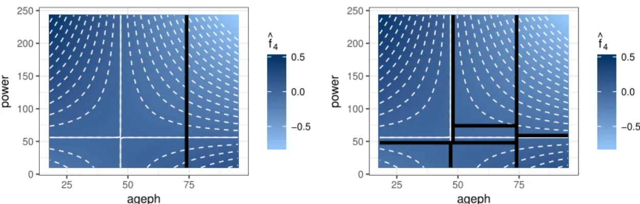
Figure 9motivates our preference for the more flexible evolutionary trees over the classic
recur-sive partitioning trees when binning the continuous risk factors. TheRpackagerpart, developed
by Therneau et al.(2015), is used to fit the recursive trees and weights are applied in the same
manner as for the evolutionary trees. The left panel of Figure9shows the first split for binning
the interaction effect. Although this split atageph= 74 is an optimal way to bin the interaction
effect in two regions, it does not imply that this split is still optimal when we bin the
interac-tion effect in three or more regions. The right panel of Figure 9 shows the binning result with
recursive partitioning for seven bins. As such we obtain the same number of bins as with the
evolutionary trees in Figure 8. Evolutionary trees lead to a much more intuitive binning result
which is globally optimal instead of only locally optimal.
0 50 100 150 200 250 25 50 75 ageph po w er −0.5 0.0 0.5 f ^ 4 0 50 100 150 200 250 25 50 75 ageph po w er −0.5 0.0 0.5 f ^ 4
Figure 9: MTPL: the optimal first split for the interaction effect (left) and the resulting seven bins for the interaction effect (right) obtained with recursive partitioning.
5 Analysis of the premium structure 20
5
Analysis of the premium structure
5.1 From GAM to GLM
We now use the categorical risk factors, as constructed in Section 4, to fit a Poisson GLM for
the frequency and a lognormal GLM for the severity of the claims data. For each risk factor we choose the bin with the largest exposure as reference class in our GLMs. A full specification of
the frequency and severity regression models is in Appendix A.
The top and bottom row of Figure10compare the original main GAM effects with the resulting
estimated GLM coefficients for the frequency and severity model respectively. Note that the
GLM coefficients of Figure10, indicated by dots, are a rescaled version of the actual coefficients.
This rescaling is performed to make the GAM effects and the GLM coefficients comparable.
Indeed, a GAM effect - for example ˆf1(ageph) - is estimated in such a way that the weighted
mean of the smooth effect, with the number of policyholders as weights, is equal to zero:
Pmax(ageph)
i=min(ageph)wagephi
ˆ
f1(agephi) Pmax(ageph)
i=min(ageph)wagephi
= 0 (12)
withwagephi the number of policyholders withageph=iand ˆf1(agephi) the corresponding fitted
GAM effect. For a categorical risk factor, the GLM coefficient for the reference class is equal to zero and the GLM coefficients of the other classes are expressed relative to this reference class. The weighted mean of the GLM coefficients, with the number of policyholders as weights, therefore depends on the choice of the reference class. We adjust the GLM coefficients such that the weighted mean of the rescaled GLM coefficients is equal to zero:
˜ βagephj = ˆβagephj − Pkageph j=1 magephjβˆagephj Pkageph i=j magephj (13)
with kageph the number of bins for the risk factor ageph, magephj the number of policyholders
in bin j and ˆβagephj the fitted GLM coefficient for the policyholders in bin j. This rescaling is
of course only performed to enable a visual comparison between the GAM effects and the GLM coefficients; the actual GLM is not adjusted in any way.
The piecewise constant functions formed by the GLM coefficients in Figure 10 approximate the
smooth GAM effects very closely, especially for bins with high exposure. For example, the GLM
coefficients for age bin [33,51) approximate ˆf1(ageph) very well. This indicates that our resulting
GLMs are a good approximation of the original GAMs. We trade flexibility for simplicity
and some discrepancies are therefore impossible to avoid. For example: both ˆf1(ageph) and
ˆ
g1(ageph) are underestimated by the GLM coefficients for the youngest and oldest policyholders.
Such discrepancies only occur in the extreme ends of the range of the risk factors, where the exposure is very low, and therefore few policyholders are affected by this.
Figure 11 shows the GAM interaction effect between agephand power in the frequency model
together with the approximation obtained with the GLM coefficients. The plus-shaped (+) region can be interpreted as a neutral zone while the top left and bottom right (bottom left
and top right) indicate regions of increased (decreased) risk. Figure 12 shows both the GAM
estimate for the spatial effect in the frequency model and its approximation in the GLM. As expected, the GLM coefficients reflect the riskiness as captured by the spatial effect from the GAM.
−0.25 0.00 0.25 0.50 25 50 75 ageph f ^ 1 −1 0 1 2 0 50 100 150 200 250 power f ^ 2 0.0 0.4 0.8 0 5 10 15 20 bm f ^ 3 0.0 0.4 0.8 1.2 20 40 60 80 ageph g^1 −0.50 −0.25 0.00 0.25 0 5 10 15 20 bm g^2
Figure 10: MTPL: comparison between the GAM effects and GLM coefficients. Top row: risk factors
ageph,bmandpowerin the frequency model. Bottom row: risk factorsagephandbmin the severity model. 0 50 100 150 200 250 25 50 75 ageph po w er −0.5 0.0 0.5 f ^ 4 0 50 100 150 200 250 25 50 75 ageph po w er GLM coefficients −0.07 −0.021 0 0.035 0.064
Figure 11: MTPL: comparison between the GAM effect and GLM coefficients for the interaction between
ageph andpowerin the frequency model.
−0.4 −0.2 0.0 0.2 f ^ 5 GLM coefficients −0.329 −0.204 −0.155 0 0.199
Figure 12: MTPL: comparison between the GAM effect and GLM coefficients for the spatial effect in the frequency model.
5 Analysis of the premium structure 22
5.2 A comparative analysis
Table7compares the statistical performance of the original GAMs and the resulting GLMs via
both the AIC and BIC measures. The GAMs attain a lower AIC value for both the frequency and severity models, whereas the GLMs attain a lower BIC value for both the frequency and severity models. This comparison clearly shows the trade-off between flexibility and simplicity in the modeling process. GAMs are the preferred tool for flexibility based on the low complexity penalty of AIC, while GLMs are the preferred tool for simplicity based on the high complexity penalty of BIC.
AIC Frequency Severity
GAM 124 630 65 593
GLM 124 643 65 603
BIC Frequency Severity
GAM 125 121 65 706
GLM 124 924 65 696
Table 7: MTPL: a comparison of statistical performance between the original GAMs and resulting GLMs via both the AIC and BIC measures.
We calculate the pure premiumπi for every policyholderias the product of the expected values
of the frequency Fi and the severity Si: πi = E[Fi]×E[Si], taking the actual exposure and
risk factors of insured i into account. We use the GAM (resp. GLM) frequency and severity
models to obtain the GAM (resp. GLM) premium structure. By summing these premiums over
all policyholders we obtain the total pure premium inflow: Π = Pn
i=1πi. At portfolio level,
the GLM and the GAM result in a pure premium cash inflow of 29 867 565 and 29 865 859 Euro respectively. The GLM premium inflow is 1706 Euro higher compared to the GAM inflow, but this difference represents only 0.006% of the total pure premium income. An insurance company therefore obtains nearly the same cash inflow by using any of the two models. The premium inflow is in both cases sufficient to cover the actual losses in the portfolio, which amount to 26 464 970 Euro. Note that policyholders with very large losses are excluded from
this comparison in order to stay in line with the modeling process as outlined in Section3.2.
Figure 13 shows a comparison between the annual GLM and GAM pure premiums by setting
exp = 1 for all policyholders in the insurance portfolio. The policyholders are ordered, from
left to right, according to increasing GAM premium in the top panel. We observe that the GLM premiums (light blue) are scattered around the GAM premiums (dark blue), but both show the same increasing trend. Differences between both premiums for a specific policyholder are attributable to differences between both the underlying frequency as well as severity models.
The bottom left panel in Figure13shows violin plots of both the GLM and GAM premiums. We
can clearly observe that the premiums resulting from both models are very similar. There is no visual difference in the bodies of both distributions. This indicates that, on average, there is no difference in premiums for the bulk of the policyholders. Our findings are confirmed by examining
the relative pure premium differences, defined as (πGLM
i −πGAMi )/πiGAM, in the bottom right
panel of Figure 13. A negative (positive) difference therefore indicates that the policyholder
pays less (more) under the GLM compared to the GAM. The differences are centered around zero, again indicating that policyholders, on average, pay the same premium in the GLM and GAM case. Note that the difference in both premiums lies between -4.7% and 5.3% for half the insurance portfolio and that the median difference is equal to 0.16%.
Figure 13: MTPL: comparison between the GAM and GLM pure premiums.
Figure 14 shows the distribution of the relative premium difference over the continuous risk
factors ageph, power and bm. The dots indicate the average of the relative differences for
policyholders with that specific risk characteristic while the error bars indicate plus and minus two times the standard deviation. The top panel shows that for most ages the premium difference is close to zero. Both very young and very old policyholders pay less under the GLM compared
to the GAM, which is in line with our findings in Figure 10. The middle panel indicates that
policyholders driving a car with low (high) horsepower pay more (less) under the GLM compared to GAM, while for the other policyholders the premium difference is close to zero, again in line
with our findings in Figure 10. The bottom panel shows that for nearly every bm level the
premium difference is close to zero. The GLM coefficients approximate the GAM effects very
closely for the low bmlevels and the approximation errors of the frequency and severity models
offset each other for high bm levels. For all continuous risk factors we can conclude that the
premium differences are close to zero in areas containing a large number of policyholders (cfr.
Figure 2).
For solvency purposes it is very important to hold enough capital such that the insurance company can fulfill its obligations towards its policyholders. We simulate 5 000 000 GLM and GAM scenarios by sampling observations from the estimated Poisson and lognormal distributions
for frequency and severity respectively. The left panel of Figure15shows the distribution of the
portfolio losses in these scenarios for both the GLM and GAM. These distributions look very similar, indicating that both models predict similar portfolio losses. The right panel of Figure
15 shows the high empirical quantiles of these losses, from the 90% quantile onwards. These
high quantiles can be interpreted as a Value at Risk (VaR), a very popular measure to calculate capital requirements. We observe that the GLM and the GAM approach result in very similar
values for the VaR. Table 8 shows the numerical values for the VaR measure at four often used
quantiles. The GLM results in slightly higher capital requirements than the GAM in three out
6 Conclusions 24 −0.50 −0.25 0.00 0.25 25 50 75 ageph Relativ e diff erence −0.5 0.0 0.5 0 50 100 150 200 250 power Relativ e diff erence −0.2 −0.1 0.0 0.1 0.2 0 5 10 15 20 bm Relativ e diff erence
Figure 14: MTPL: distribution of the premium differences over the continuous risk factorsageph,power
andbm. 3.0e+07 3.5e+07 4.0e+07 4.5e+07 GLM GAM Sim ulated losses 3.10e+07 3.15e+07 3.20e+07 3.25e+07 0.900 0.925 0.950 0.975 1.000 Quantile V aR Model GLM GAM
Figure 15: MTPL: comparison of the simulated losses and empirical quantiles under the GAM and GLM.
VaR 95% 99% 99.5% 99.9%
GAM 31 064 090 31 641 996 31 875 657 32 449 219
GLM 31 066 851 31 644 391 31 878 921 32 448 961
Table 8: MTPL: comparison of the 95%, 99%, 99.5% and 99.9% VaR for the GAM and GLM.
6
Conclusions
This paper presents a fully data driven strategy to bin spatial and continuous risk factors with the goal of deploying these in a practical insurance tariff. We develop a predictive model for claim frequency as well as severity. Combining both these models allows the actuary to calculate a pure risk premium for an insurance contract. We start from the framework of generalized additive models and build close approximations to these models. As such an easy to understand predictive model results which is formulated within the well-known framework of generalized linear models.
Starting from a GAM with flexible effects for continuous risk factors, their interactions and a spatial effect, we propose to bin the spatial effect using Fisher’s natural breaks algorithm and the effects of the continuous risk factors using evolutionary trees.
Fisher’s natural breaks method minimizes the within-bin variance and hence results in a
homo-geneous binning of the spatial effect. This method is very similar to the K-means clustering
algorithm (see MacQueen et al.,1967), though uses dynamic programming and will always
re-turn the same (optimal) binning result. K-means starts optimizing after a random initialization
and the end result therefore depends on this initialization. Fisher’s method is only applicable
to one-dimensional binning problems whereas K-means generalizes towards higher dimensional
settings. This is not a problem in our case since binning the spatial effect is a one-dimensional problem.
The evolutionary trees are very good at binning the main effects of continuous risk factors. They focus on splitting a smooth effect in ranges where it has a large slope, but only if sufficient policyholders are present in these ranges. As such, the composition of the current portfolio is taken into account and our approach will automatically adapt to changing portfolio composi-tions. The evolutionary trees also perform well at discriminating between areas of increased and decreased risk in a two-dimensional setting for interaction effects of continuous risk factors. In our case study, this leads to a neutral zone grouping policyhoders with very similar risk profiles and regions containing policyholders with increased or decreased risk profiles. A downside of using a single regression tree to split a bivariate interaction effect is the fact that the resulting bins will always have a rectangular shape. It is therefore not possible to produce a split along
a non-linear contour line such as those encountered in Figure 4. More complex models - for
example boosted trees or support vector machines - are needed to obtain non-linear borders. The problem with such models however is their lack of interpretability; a non-linear border is harder to explain than the straight borders produced by a regression tree.
Our approach leads to GLMs which involve a simpler tariff structure compared to the original GAMs. We observed that premiums, expected losses and capital requirements calculated from the resulting GLM approximate those calculated from the original GAM quite closely. We therefore end up with a simpler model that can be deployed in practice as a close substitute for a more complex, flexible model.
The application of our approach is not limited to the case of car insurance or P&C insurance in general. It can be used in every business environment where it is useful to approximate flexible smooth effects with more interpretable and simpler predictive models that are easier to explain to stakeholders. An obvious example is credit scoring, since a credit scoring model needs to be transparent and easy to explain to customers.
Our paper illustrates the use of data analytics within insurance pricing. This field is rapidly gaining importance in the era of big data. We focus on the interplay between the traditional toolkit of the pricing actuary (e.g. GLMs) and tools from the machine learning community (e.g. regression trees and genetic algorithms). We illustrate the complementarity of these tech-niques in pricing practice and how they can assist an actuary in finding the right balance between flexibility and simplicity.
Acknowledgements
We would like to thank Michel Denuit for providing the data and for his valuable suggestions. Furthermore, the authors acknowledge financial support from the Ageas Continental Europe Research Chair at KU Leuven and from KU Leuven’s research council (project COMPACT C24/15/001).