Comparative Validation of Polyp Detection Methods
in Video Colonoscopy: Results from the MICCAI
2015 Endoscopic Vision Challenge
Jorge Bernal
∗, Nima Tajkbaksh
∗, F. Javier Sánchez, Bogdan J. Matuszewski, Hao Chen, Lequan Yu, Quentin
Angermann, Olivier Romain, Bjørn Rustad, Ilangko Balasingham, Konstantin Pogorelov, Sungbin Choi, Quentin
Debard, Lena Maier-Hein, Stefanie Speidel, Danail Stoyanov, Patrick Brandao, Henry Córdova, Cristina
Sánchez-Montes, Suryakanth R. Gurudu, Gloria Fernández-Esparrach, Xavier Dray, Jianming Liang
+, Aymeric
Histace
+Abstract—Colonoscopy is the gold standard for colon cancer screening though still some polyps are missed, thus preventing early disease detection and treatment. Several computational systems have been proposed to assist polyp detection during colonoscopy but so far without consistent evaluation. The lack of publicly available annotated databases has made it difficult to compare methods and to assess if they achieve performance levels acceptable for clinical use. The Automatic Polyp Detection sub-challenge, conducted as part of the Endoscopic Vision Challenge (http://endovis.grand-challenge.org) at the international confer-ence on Medical Image Computing and Computer Assisted Intervention (MICCAI) in 2015, was an effort to address this need. In this paper, we report the results of this comparative eval-uation of polyp detection methods, as well as describe additional experiments to further explore differences between methods. We define performance metrics and provide evaluation databases that allow comparison of multiple methodologies. Results show that convolutional neural networks (CNNs) are the state of the art. Nevertheless it is also demonstrated that combining different methodologies can lead to an improved overall performance.
Index Terms—Endoscopic vision, Polyp Detection, Hand-crafted features, Machine Learning, Validation Framework
∗Authors contributed equally to this work,+Last position is shared between
the authors.
Jorge Bernal and F. Javier Sánchez are with Computer Science Department at Universitat Autònoma de Barcelona and Computer Vision Center, Spain
Nima Tajkbaksh and Jianming Liang are with Arizona State Univ., USA Aymeric Histace, Quentin Angermann, Olivier Romain and Xavier Dray are with ETIS, ENSEA, Univ. of Cergy-Pontoise, CNRS, Cergy, France. Xavier Dray is also with Lariboisière Hospital-APHP, France.
Hao Chen and Lequan Yu are with Dpt of Computer Science and Engi-neering, Chinese University of Hong Kong, China
Bjørn Rustad and Ilangko Balasingham are with Oslo University Hospital. Bjørn Rustad is also with OmniVision, University of Oslo, Norway.
Konstantin Pogorelov is with Media Performance Group, Simula Research Laboratory and University of Oslo, Norway
Sungbin Choi is with Seoul National University, Seoul, South Korea Bogdan J. Matuszewski is with School of Engineering, University of Central Lancashire, Preston, United Kingdom
Quentin Debard is with University of Nice-Sophia Antipolis, Nice, France Lena Maier-Hein is with the junior group Computer-assisted Interventions, German Cancer Research Center (DKFZ), Germany
Stefanie Speidel is with the Institute for Anthropomatics, Karlsruhe Institute of Technology, Germany
Danail Stoyanov and Patrick Brandao are with the Centre for Medical Image Computing and Dept. of Computer Science, Univ. College London, UK
Henry Córdova, Cristina Sánchez-Montes and Gloria Fernández-Esparrach are with Endoscopy Unit, Gastroenterology Department, Hospital Clínic, IDIBAPS, CIBEREHD, University of Barcelona, Barcelona, Spain
Suryakanth R. Gurudu is with Division of Gastroenterology and Hepatol-ogy, Mayo Clinic, Scottsdale, Arizona, USA
Copyright (c) 2010 IEEE. Personal use of this material is permitted. However, permission to use this material for any other purposes must be obtained from the IEEE by sending a request to [email protected].
I. INTRODUCTION
This paper introduces the results and main conclusions of the MICCAI 2015 Sub-Challenge on Automatic Polyp Detection in Colonoscopy, conducted as part of theEndoscopic Vision Challenge (http://endovis.grand-challenge.org). More precisely, we present a validation study comparing the perfor-mance of different polyp detection methods covering different methodologies proposed by participating teams, providing an insight analysis of their detection yield. In this section, we introduce both clinical and technical contexts.
A. Clinical context
Colorectal cancer (CRC) is the third largest cause of cancer deaths in the United States among men and women, and it is expected to have resulted in about49,196deaths in 2016 in the USA [1]. CRC arises from adenomatous polyps (or adenomas), that are growths of glandular tissue originating from the colonic mucosa. Though adenomas are initially benign, they might become malignant over time and spread to adjacent and distant organs such as lymph nodes, liver or lungs, being ultimately responsible for complications and death [2].
CRC prevention is first based on the detection of at-risk patients: those with symptoms (such as hematochezia and anemia), those with positive screening tests (such as a fecal occult blood test or a fecal immunochemical test), and those with a past history of adenoma or with a family history of advanced adenoma or CRC. In these groups of patients, a colonoscopy is proposed to detect polyps before any malignant transformation or at an early cancer stage. This stage refers to the most superficial colon layers, with no deep invasion, and it is associated with a 5-year survival rate over 90%[3], [1]. If any polyp found is characterized as a likely adenoma, its removal should be considered to confirm the diagnosis, to set its histological stage and to confirm its complete removal, giving clinicians clues to determine the need and timing of the next colonoscopy [4].
Though colonoscopy is the gold standard for colon screen-ing, other alternatives, such as CT colonography [5] or wireless capsule endoscopy (WCE) [6], are also used to search for polyps. They are less invasive to patients and do not present perforation risk. Though, as colonoscopy, they require bowel preparation. Nevertheless in these cases, if a polyp is found, a colonoscopy must be considered to remove the suspicious
lesion. These alternatives have specific limitations that may affect the outcome of the screening. For instance, CT colonog-raphy has a low small lesions (5 mm or less) detection rate due to resolution constraints [7] and it implies using ionising radiation. WCE allows to detect all kind of lesions but their observation depends on whether they are recorded during the progress of the camera through the gastrointestinal tract or not. Moreover, its diagnostic yield is highly dependent on the cleanliness of the colon (whereas colonoscopy has some in-situ lavage capabilities). Last but not least, the analysis of the information provided by WCE can be highly time-consuming, as the recorded videos can last up to 8 hours [8].
Colonoscopy presents some drawbacks, polyp miss-rate being the most important among these. Colonoscopy rarely misses polyps bigger than 10mm, but the miss-rate increases significantly with smaller sized and/or flat polyps [9], [10]. It has also to be noted that colonoscopies are seldom recorded, so a new procedure must be performed to revisit explored areas. The outcome of the colonoscopy exploration depends on: 1) bowel preparation [11]; 2) specific choice of endoscope and video processor, affecting image quality and preventing the use of certain image enhancing tools; 3) clinicians’ skills, as both endoscopist’s experience and his/her actual concentration during the intervention may influence the degree of procedure completion (reaching the cecum or not) and the percentage of the colon that has been explored [12], [13] and 4) patient-specific issues, as due to colon movements and the appearance of folds and angulations during the exploration, some parts of the colon which may potentially present polyps may not be reached [9]. Moreover, patients’ personal and family history can increase the risk of having a polyp and, in this case, the exploration should be even more thorough.
B. Technical strategies to improve polyp detection rate
Apart from the continuous improvement of clinicians’ skills through training programs and practice [14], technical efforts are being undertaken to improve colonoscopy’s outcome. We clustered them into two groups: improvement of devices and the development of computational support systems.
Amongst the device improvements, the following should be highlighted: 1) increase in image resolution and, consequently, textural information; 2) the use of wide-angle cameras showing more colon wall surface; 3) the development of zooming and magnification techniques [15] and 4) the development of new imaging methodologies such as autofluorescence imaging [16] or virtual chromoendoscopy (Olympus’ Narrow Band Imaging [17], Fujinon’s FICE [18] or Pentax’s i-Scan [19]). This last group of techniques modify how the scene is observed by improving the contrast of endoluminal scene elements, which may help in lesion detection and also with in-vivo lesion diagnosis due to the enhanced visualization of lesion tissues [20]. These advances have fostered the cooperation between clinicians and computer scientists in the development and validation of computer-aided support systems for colonoscopy, aimed to help clinicians in all stages of CRC diagnosis. A significant part of this effort has been focused on computer assisted polyp detection. As it is indicated in [21], cooperation
between technologists and clinicians is essential to develop clinically useful solutions, with both these groups understand-ing challenges and limitations in their respective domains.
Automatic polyp detection in colonoscopy videos has been an active research topic during the last 20 years and several approaches have been proposed. We present a review of the most relevant methods in Section II but, to the best of our knowledge, none of them has been adopted for a routine patient treatment. There might be several reasons behind this. First of all, in order for a given method to be clinically useful, it has to meet real time constraints; e.g. for videos acquired at 25 frames per second (fps) the maximum time available to process each image frame should be under 40ms. Secondly, some of them are built from a theoretical model of a polyp appearance [14], [22] and therefore limited to only certain polyp morphologies, which may not translate to the actual scene where polyp appearance varies greatly. Thirdly, the majority of methods are mainly focused on the polyps and they do not consider the presence of other elements such as folds, blood vessels or the lumen that can affect methods’ performance [14]. Last but not least, some of these methods have been only trained and tested on selected good quality still image frames. The lack of temporal coherence and the great variability in polyp appearance due to camera progression and visibility conditions might impact their performance in the full sequences analysis, as they might cause instability in their response against similar stimuli.
Computational methods also have to deal with additional colonoscopy-specific challenges. For instance, they should consider the impact of image artifacts generated due to scene illumination (specular highlights, overexposed regions) or to specific configuration of the videoprocessor attached to the colonoscope, which might overlay information over the scene view. These artifacts, apart from altering the view of the scene, might not be stable within consecutive frames and therefore methods should both compensate their impact on the individual frame polyp detection and tracking in the full sequence analysis. Additionally, though an effort is made to ensure an adequate bowel preparation, some particles may still appear which, in some cases, could lead to false detections when isolated or to occlusion leading to miss detection or localization errors. As mentioned before, these methods have to cope with a great degree of variability in polyp appearance which depends on illumination conditions, camera position and on clinician skills when progressing through the colon. Finally, available methods have been typically validated on small and restricted databases, under specific endoscope device conditions (brand and resolution), in some cases even covering only one specific polyp type, shape or morphology hindering their actual performance in a more generic setting.
C. Motivation of the comparison study
Unfortunately, the lack of a common validation framework, which is a frequent problem in medical and endoscopy image analysis [21], has limited the effectiveness of the comparison between existing approaches, making it difficult to determine which of them could have actual advantage in clinical use.
To cope with this, efforts have been made on publishing fully annotated databases [14], [22] and on organizing challenges as part of international conferences (ISBI, MICCAI), which offer a basis to discuss validation strategies.
Considering this and taking inspiration from recent works on quantitative comparative methods’ analysis in areas such as laparoscopic 3D Surface Reconstruction [23] or liver seg-mentation [24], we present in this paper a complete validation study of polyp detection methods performed as part of the 2015 MICCAI sub-challenge on Automatic Polyp Detection. This sub-challenge was organized jointly by three research teams: 1) Computer Vision Center/Universitat Autònoma de Barcelona and Hospital Clinic from Barcelona, Spain (CVC-CLINIC); 2) ETIS Lab (ENSEA/CNRS/University of Cergy-Pontoise) and Lariboisière Hospital-APHP at Paris, France (ETIS-LARIB), and 3) Arizona State University and Mayo Clinic, USA (ASU-Mayo).
The objective of this paper is to present a comparative study of polyp detection methods under a newly proposed validation framework. This validation framework was firstly introduced as part of MICCAI 2015 Sub-Challenge on Automatic Polyp Detection in Colonoscopy and we present in this paper the results of the mentioned sub-challenge. Beyond this, we also propose additional experiments to assess even more in-depth the performance of an automatic polyp detection method. These new experiments are focused on exploring the actual clinical applicability of a given method by assessing up to what extent they are affected by some of the technical and clinical challenges reported in the literature or whether they incorporate temporal coherence features or not. Finally we also go beyond the individual analysis of methods and propose combination strategies in order to study whether a combination method may lead to improved individual performance.
The remainder of the paper is structured as follows: In Section II we present the methods proposed by each of the participating teams in the challenge, including them in the context of existing published methods. In Section III we describe the complete validation framework. Results from the comparative study are presented in Section IV. Section V provides an in-depth analysis of the results and discusses some topics related to challenge organization. Finally, the concluding remarks are drawn in Section VI.
II. AUTOMATICPOLYPDETECTIONMETHODS
A. Historical review of computational polyp detection methods
After analyzing approaches reported in the literature, we propose to cluster methods into three groups: 1) hand-crafted; 2) end-to-end learning and 3) hybrid approaches. This taxonomy represents the different historical trends of polyp detection methods, as in early 2000s, the majority of the methods used a given texture descriptor to guide a classification method but, subsequently, some researchers decided to go for hand-crafted features, aiming at a real time implementation. As technology evolved and the computational capabilities increased, techniques such as neural networks that were developed in the past and abandoned due to excessive computational cost have now resurfaced.
Regarding hand-crafted methods, the majority are based on exploiting low-level image processing methods to obtain candidate polyp boundaries (using Hessian filters in the work of Iwahori et al. [25], intensity valleys in the work of Bernal et al. [14] or Hough transform in the work of Silva et al, [26]) and then use resulting information to define cues unique to polyps. For instance, the work of Zhu et al. [27] analyzes curvatures of detected boundaries whereas the method of Kang et al. [28] is focused on searching ellipsoidal shapes typically associated with polyps. Finally, the method of Hwang et al. [29] combines curvature analysis and shape fitting in their strategy.
Concerning end-to-end learning, texture and color informa-tion were formerly used as descriptors such as in the work of Karkanis et al. [30] which proposed the use of color wavelets, the work of Ameling et al. [31] that exploits the use of co-ocurrence matrices or the work of Gross et al. [32], which proposed the use of local binary patterns. Active learning methodologies have also been introduced as in the work of Angermann et al. [33] to reinforce the tradeoff between performance and computation time. Some of the most recent methods use deep learning tools to aid in polyp detection tasks, as in the work of Park et al. [34] or in the work of Ribeiro et al. [35]. In these very recent developments, differences among methods are based on the selection of a specific network architecture and databases used for training.
Finally, there are several hybrid methods which combine both methodologies for polyp detection, such as in the works of Tajbaksh et al. [22], which combines edge detection and feature extraction to boost detection accuracy, the work of Bae et al. [36], that propose a system based on imbalanced learning and discriminative feature learning; the work of Silva et al. [26], which uses hand-crafted features to filter non-informative image regions and the work of Ševo et al. [37], which combines edge density and convolutional networks.
As mentioned in Section I, the great majority of the methods are tested on private databases though we can observe that more recent publications such as the work of Park et al. [34] or the work of Ribeiro et al. [35] have started to use publicly available databases such as the ones used in the MICCAI 2015 Sub-challenge on Automatic Polyp Detection. Related to this, apart from new proposals, some of the referenced methods have been adopted by participants, such as the works of Bernal et al. [14], Silva et al. [26] or the work of Tajbaksh et al. [22]. We provide in the next subsection a brief description of participating methods highlighting their most relevant contributions to the field. We grouped the methods following the taxonomy defined earlier in this subsection.
B. MICCAI 2015 Polyp Detection Sub-challenge methods 1) Hand-crafted features:
• CVC-CLINIC: This method [14] is based on a model of appearance considering polyps as protruding surfaces, being their boundaries defined from intensity valleys detection. Their proposal includes a pre-preprocessing stage to mitigate the impact of other valley-rich structures (blood vessels, specular highlights). To build final energy maps highlighting polyp presence, four different
TABLE I
SUMMARY OF INFORMATION FROM THE TEAMS THAT TOOK PART INMICCAI 2015 CHALLENGE ONAUTOMATICPOLYPDETECTION.
Team
acronym Full team details Methodology Published
Still-frame analysis Video analysis Training (seconds) Testing
(seconds) System tested
ASU Arizona State University (USA) Hybrid Yes [22] No Yes N/A 2.7
2.4 GHz Intel quad core processor and an NVIDIA GeForce GTX 760 video card CUMED
Department of Computer Science and Engineering, Chinese Uni-versity of Hong Kong (China)
End-to-end learning (CNNs) No Yes Yes 10800 0.2 A standard PC with a 2.50 GHz Intel(R) Xeon(R) E5-1620 CPU and a NVIDIA GeForce GTX Titan X GPU CVC-CLINIC
Computer Vision Center and Universitat Autònoma de Barcelona (Spain)
Hand-crafted Yes [14] Yes Yes N/A 10 Intel core i7-4790 at 3.6GHz
ETIS-LARIB
ETIS, ENSEA, University of Cergy-Pontoise, CNRS, Cergy (France)
Hybrid Yes [26] Yes No 196 2.14 Intel i5 4200U 2.30 GHz OUS
Oslo University Hospital, OUS Norway, University of Oslo (Norway)
End-to-end learning (CNNs)
No Yes Yes 86400 5
Intel i5, 4 cores at 2.8 GHz, 4 GB RAM. Graphic card with 4 GB memory used for training PLS
Polyp Localize and Spot Team, Media Performance Group, Sim-ula Research Laboratory and University of Oslo (Norway)
Hybrid No Yes Yes 0.33per image 0.145
2 Intel(R) Xeon(R) CPU E5-2650 at 2.00GHz CPU, 64 GB of RAM, NVIDIA Corporation GK110, GeForce GTX TITAN
SNU Seoul National University, Seoul (South Korea)
End-to-end learning (CNNs)
No Yes Yes 360 0.8-1 NVIDIA TITAN X GPU
UNS-UCLAN
School of Engineering, Uni-versity of Central Lancashire, Preston (UK) and University of Nice-Sophia Antipolis, Nice (France) End-to-end learning (CNNs) No Yes No 18000 5 i7-5930K @ 3.5GHz (6 cores), 64 GB RAM, NVIDIA GeForce GTX TITAN X
constraints (continuity, completeness, concavity, and ro-bustness against spurious structures) are imposed to candidate boundaries to differentiate polyps from other structures.
2) End-to-end learning:
• CUMED:The architecture of the proposed network
con-tains two sections including a downsampling path and an upsampling path [38]. The former contains convolutional and max-pooling layers while the latter contains convo-lutional and upsampling layers, increasing the resolutions of feature maps and output prediction masks. To alleviate the problem of vanishing gradients and encourage the back-propagation of gradient flow in deep neural net-works, the auxiliary classifiers are injected to train the network. Furthermore, they can serve as regularization to reduce over-fitting and improve the discriminative capability of features in intermediate layers [39], [40]. The classification layer, after fusing multi-level contex-tual information, produces the detection results. Network training is formulated as a pixel-wise classification prob-lem with respect to ground-truth masks. The highlight of this approach is that it explores multi-level feature repre-sentations with fully CNNs in an end-to-end way, taking an image as input and directly providing the score map. In addition, feature-rich hierarchies from a large scale auxiliary dataset are transferred into the model to reduce over-fitting and further boost detection performance [41].
• UNS-UCLAN:This method, inspired by reported works [42], [43], [44], uses three CNNs trained at different image scales, namely 1, 0.5, and 0.25, of the original training images. For all the scales the CNNs use the same architecture, but they are trained independently on
the RGB images at their corresponding scale. After this initial training phase, the last fully connected part of each CNN is removed and the outputs from the ’convolutional part’ of all the three networks are fed as input to a single Multi-Layer Perceptron (MLP) network. This additional network is trained independently from the three CNNs. In this approach CNNs are used as feature extraction engines operating at different spatial scales, and the MLP performs the classification based on these features. The method’s output is the polyp incidence probability map, which is then processed to locate dominant prob-ability peaks, as peaks locations and probprob-ability values are returned as the final output of the system. The training was performed exclusively on the CVC-CLINIC database.
• OUS: This method is based on the popular AlexNet model [44] for CNNs and its slight modification Caf-feNet, which is pre-trained on the ILSVRC 2012 [45] dataset. Computations are achieved using the Caffe li-brary [46]. The original model is modified to take input patches of size 96× 96, and the kernel size of the two first pooling layers is decreased from 3 to 2, while the last pooling layer is removed. The output layer is modified to give two outputs, polyp or non-polyp. In order to increase the training examples, data augmentation is performed in the form of random mirroring, rotation, up-and down-scaling, cropping, up-and brightness adjustment. Final polyp presence or absence was determined by using a sliding-window strategy, with three scalings for still frame analysis and two for full video sequence analysis.
• SNU: This methodology proposes a two-step approach: detection and localization. For both steps, CNNs were
used. Starting from GoogleNet (pre-trained on the Ima-geNet dataset), a CNN fine-tuning was performed. Input image is resized to 224x224 pixels prior training and data augmentation (rotation and scaling) is also performed. Training set images are augmented by using several degrees of random rotation and scaling. Detection is con-sidered as a simple binary classification task whereas, for localization, CNN are applied on polyp-positive images which are then segmented into a uniform-sized 8x8 grid (64 grids per image). Then, for each image, one grid is overlaid in black and then CNNs are applied thereafter to perform the binary classification task. The 64 overlaid grid images are then sorted by classification score to calculate final polyps’ position.
3) Hybrid approaches:
• PLS: The proposed full localization scheme consists of
two parts, detection and localization. Regarding detec-tion, two sets of images, one containing polyps, and the other without polyps, are used for training. Global image features [47] are used as they are easy and fast to calculate. Based on similarity scores between input frame and training ones and results ranks, the detection subsystem decides in real-time to which class (polyp or no polyp) the input frame belongs to.
The localization scheme is implemented as a sequence of preprocessing filters (RGB to YCbCr color space conver-sion, removal of borders and sub-images, flare masking and low-pass filtering) and uses the polyp’s physical shape to find its exact position, approximating polyps by elliptical shape regions presenting local features that differentiate them from surrounding tissues. The final decision regarding polyp location is taken by means of the maximum values in the energy map computed using the elliptical shape of the polyp’s usual appearance. Finally, the method outputs four possible locations per frame.
• ETIS-LARIB : This method [26] is inspired by the psycho-visual methodology used by clinicians when per-forming an endoscopic examination. First, a detection of the Regions of Interests (ROI) that may contain a polyp is performed using shape and size image features. This first pre-selection allows a first and fast scanning of the image. Due to being circular/elliptical shapes associated to polyps, a Hough transform was used for this first filtering stage. Once ROIs are detected, a second analysis, based on texture is achieved in order to remove those ROIs with no actual polyp content. To achieve this, an ad-hoc classifier based on a boosting-based learning pro-cess using texture features computed from co-ocurrence matrices (standard Haralick features) is proposed.
• ASU:This method [22] consists of two stages. In the first stage, a set of polyp candidates is generated using geo-metric features. Specifically, given a colonoscopy frame, a crude set of edge pixels is first obtained. This edge map is then refined using a classification and feature extraction scheme [48]. The goal of the edge classification scheme is to remove as many non-polyp boundary pixels as possible from the initial edge map. The geometry of the retained
edges is then used in a voting scheme that localizes polyps candidates as objects with curved boundaries in the refined edge maps. The voting scheme further estimates a bounding box for each generated candidate based on the generated voting map. In the second stage, an ensemble of CNNs -each of them specialized in one type of features- is applied to each candidate bounding box [49]. Finally, the outputs of the CNNs are averaged to generate a confidence score for a given polyp candidate. Table I shows a summary of the different methods partic-ipating at MICCAI 2015 Challenge on Automatic Polyp De-tection. As each method was tested under different conditions, computation times are given to complete the information on the training and testing processes.
III. VALIDATION STUDY
We introduce in this section the complete validation study proposed to assess and compare the performance of different polyp detection methods.
A. Definitions and general performance metrics
We define Polyp detection as the capability of a given method to determine polyp presence in a colonoscopy frame (Polyp presence detection) and, once this is determined, it is able to provide the location of the polyp within the image (Polyp localization). Consequently, a good polyp detection method should select images (video frames) containing polyps and ignore all others and it should indicate the position of all polyps present in an image. There are some terms defined next which are key to set performance metrics. As we deal with images from real patients examinations, we will find two different cases: images with polyps and images without polyps. In the first case, if detection output is within the polyp, the method is said to be providing a True Positive (TP)
or correct alarm. It has to be noted that only one TP will be considered per polyp, no matter how many detections fall within the polyp. Any detection that falls outside the polyp is considered aFalse Positive (FP) or false alarm. The absence of alarm in images with a polyp is considered aFalse Negative (FN), counting one per each polyp in the image that has not been detected. Regarding images without polyps, we define as aTrue Negative (TN)whenever the method does not provide any output for this particular image. Any detection provided for frames without a polyp counts as a False Positive (FP). Considering these definitions, we propose the use of the frame-based performance metrics presented in Table II.
TABLE II
PERFORMANCE METRICS FOR POLYP DETECTION. Metric Abbreviation Calculation
Precision Prec P rec=T PT P+F P
Recall Rec Rec=T PT P+F N
Specificity Spec Spec=F PT N+F N
F1-measure F1 F1 =2×P recP rec+×RecRec
TABLE III
CONTENT OFASU-MAYOCLINICCOLONOSCOPYVIDEO © DATABASE.
Training database Testing database
Video Length Polyp/Total [Res] Video Length Polyp/Total [Res] Video Length Polyp/Total [Res] Video Length Polyp/Total [Res] 1 22 0/682[712×480] 11 10 245/324[1920×1080] 1 19 0/599[712×480] 11 15 338/452[1920×1080] 2 27 0/838[712×480] 12 30 910/910[1920×1080] 2 20 0/625[712×480] 12 4 134/0134[1920×1080] 3 25 0/769[712×480] 13 17 374/519[1920×1080] 3 20 0/628[712×480] 13 10 312/312[1920×1080] 4 23 0/712[712×480] 14 16 391/501[856×480] 4 20 0/607[712×480] 14 60 0/1815[712×480] 5 61 0/1843[712×480] 15 36 1106/1200[856×480] 5 30 693/918[856×480] 15 59 0/1795[712×480] 6 64 0/1925[712×480] 16 11 209/339[1920×1080] 6 40 1218/1218[856×480] 16 54 0/1627[712×480] 7 51 0/1550[712×480] 17 13 234/418[856×480] 7 18 445/555[712×480] 17 60 0/1807[712×480] 8 58 0/1740[712×480] 18 18 189/259[1920×1080] 8 14 335/446[856×480] 18 61 0/1835[712×480] 9 60 0/1802[712×480] 19 20 235/616[1920×1080] 9 13 290/396[1920×1080] 10 54 0/1639[712×480] 20 13 385/410[856×480] 10 60 548/1805[1920×1080] B. Databases
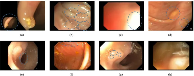
Three different databases are used in the context of the validation study presented in this paper. Two publicly avail-able databases were proposed for still frame analysis, CVC-CLINICandETIS-LARIB. CVC-CLINIC [14] contains 612 Standard Definition (SD) frames and comprises 31 different polyps from 31 sequences. ETIS-LARIB database contains 196 High Definition (HD) frames and comprises 44 different polyps from 34 sequences. More details on these databases are presented in Table IV. It has to be noted that all images contain at least a polyp; both databases were built to cover as many different polyp appearances as possible. Ground truth consisting of a polyp mask was generated using the same procedure for both databases: Images were annotated by expert videoendoscopists from the corresponding associated clinical institution. These experts (one per hospital) were asked to outline the boundaries of any polyps present in the image. These boundaries are used to generate a binary mask representing the actual polyp area within the image, also to be used for validation purposes. Examples from these two databases are shown in the first two columns of Fig. 1.
The ASU-Mayo Clinic Colonoscopy Video © Database
[22] comprises a set of short and long colonoscopy videos, col-lected at the Department of Gastroenterology at Mayo Clinic, Arizona. This database consists of 38 different, fully annotated videos. The videos were selected to display maximum varia-tion in colonoscopy procedures including different resoluvaria-tions and examination strategies (careful vs. fast inspection) and also include frames containing biopsy instruments or device information. Ground truth consisting of binary masks (polyp frames) and black frames (non-polyp frames) were created by volunteer students at Arizona State University and have been reviewed and corrected by a trained expert. Table III outlines information about the videos in that database, including for each video duration in seconds (Length), number of frames with polyps and the total number of frames (Polyp/Total) and
TABLE IV
SUMMARY OF CONTENT OF STILL FRAME VALIDATION DATABASES. SD STANDS FORSTANDARDDEFINITION, HDSTANDS FORHIGHDEFINITION.
Database Purpose Institution Content Device CVC-CLINIC Training Hospital Clinic, Barcelona, Spain 612 SD frames (388 × 284) from 31 sequences Olympus Q160AL and Q165L, Exera II videoprocessor ETIS-LARIB Testing Lariboisière Hospital, Paris, France 196 HD frames (1225× 966) from 34 sequences
Pentax 90i se-ries, EPKi 7000 videoprocessor
the image resolution (Res). An example from this database is shown in the third column of Fig. 1.
C. Statistical analysis
In order to account for statistically significant differences in performance between methods, we propose first to perform a Saphiro-Wilk test to find out whether the available data follows a normal distribution or not. In the first case (normal distribution) statistically significant differences across methods will be assessed using an analysis of variance (ANOVA) to detect differences regarding proposed metrics. In the second case (no normal distribution), the Kruskal-Wallis test will be used. All tests are done at a confidence level1−α= 0.95.
Considering the scope of the analysis presented in the paper, the metric that will be used to compare different methods will be F1-score, as it presents a balance between missed polyps and false alarms. We perform a statistical study of this metric only in videos with polyp (and potentially non-polyp) frames, as the number of samples in the still-frame analysis is not big enough to provide with statistically relevant conclusions and the analysis in videos with no polyps would cause the F1 score to be zero for all methods. We also perform statistical analysis of detection latency but, for the sake of a proper statistical comparison, this analysis is only done for those teams which detect the polyp in all sequences.
D. MICCAI 2015 Sub-challenge validation study
Two different scenarios were presented to the participants of the challenge: (i) still frame analysis and (ii) full video
(a) (b) (c)
(d) (e) (f)
Fig. 1. Illustration of the content of the CVC-CLINIC (first column), ETIS-LARIB (second column) and ASU-Mayo Clinic (third column) databases. The first column shows the original images with the corresponding reference polyp contour shown as a blue line and the second contains binary masks representing the ground truth
analysis. In the following, we present specific information of the two presented scenarios, including validation databases and performance metrics used in each of them.
1) Still frame analysis: The objective of this analysis was to explore localization capabilities of a polyp detection method. We aim to test how different methods perform in challenging high-definition (HD), high-quality images showing great vari-ability in polyp appearances. In this case, each image contains at least one polyp and images have been selected in order to have shots in which polyp appearance can be mistaken with other elements of the scene (folds, vessels).
Two different databases were used in this study: CVC-CLINICis used for thetrainingstage whereasETIS-LARIB
is used during the testing stage. Participating methods are compared using performance metrics exposed in Table II. Additionally, in case a given method provides confidence values a Precision-Recall curve is also provided otherwise the operating point will represent its performance.
2) Video analysis: In this second scenario we aim to explore full polyp detection capabilities (localization and pres-ence detection) of a given method in full sequpres-ences from actual colonoscopy procedures. In this case, polyp detection methods have to deal, apart from appearance variability, with potential polyp presence or absence in each image and, moreover, with variability in image quality (blurring, bowel preparation). Additionally, the videos in the second scenario may contain images with extra-endoluminal elements such as device information or surgical instruments. We also have to consider that, as in real procedures, nor all the sequences or all the frames contain a polyp.
The ASU-Mayo Clinic Colonoscopy Video © Database
was used in this experiment. Apart from using common performance metrics exposed in Table II, we proposed an additional performance metric to assess whether how fast a given detection method reacts to polyp presence. In this context,Detection Latency (DL): DL=f irst_detection−
f irst_appearance represents the delay in frames between the first appearance of the polyp in the video sequence (f irst_appearance) and the first actual detection of the polyp by a method (f irst_detection). Considering this, a clinically useful support system should have a DL close to zero. Finally we also provide with Receiver Operating Curves (ROC), though again, each method’s representation depends on whether they provide detections’ confidence values or not. From a general organization perspective, all teams taking part in the challenge were to use the same data for both their training and testing stages. Participants were provided with labelled training data on June 15th whereas unlabelled testing data (still frames and full sequences) was released on July 24th. In order to take part in the challenge, each participating team was asked to provide a unique CSV file for the analysis of the ETIS-LARIB database and/or one CSV file for each of the 18 testing videos in the ASU-Mayo database, depending on the sub-category the team would take part in. Each row in the CSV file represents a detection candidate region. Additionally, teams could also provide a confidence value (value between 0 and 1) for the performance curves drawing purposes, though this was not mandatory. Finally, though 8 different teams
(a) (b) (c)
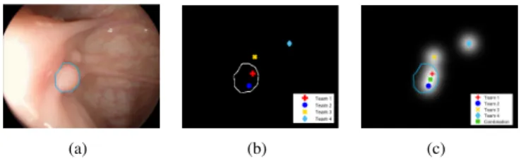
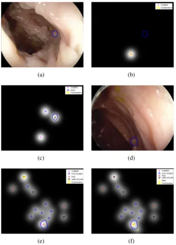
Fig. 2. Synthetical examples of different ways to perform a combination of methods: (a) original image; (b) result of combination by union, and (c) result of combination by saliency map creation. Outputs from different teams are represented by different colors and shapes. In all images, the contour of the polyp is represented as a blue curve.
took part in the challenge, not all of them participated in all categories. ASU did not take part in the still-frame analysis sub-category whereas ETIS-LARIB and UNS-UCLAN did not take part in the video analysis one.
E. Additional validation experiments
1) Combination of methods: In this study we propose to go beyond the analysis of individual methods by providing quan-titative elements on how potential combinations of some of the presented approaches may lead to an improved performance. Inspired by [50], we have studied two options of fusing the methods, namely: 1)combination by union and 2)saliency mapcreation.
The first one consists of adding, for a particular frame, the outputs from all submitted methods. Saliency maps creation proposes a combination of the output of the methods in order to generate heat maps which aim to represent those areas in the image where most of the methods coincide in their decision regarding polyp location, following the methodology proposed in [14]. We show in Fig. 2 a graphical comparison between both strategies.
In this case, we treat the output of each method as a ’fixation’ or vote, and we create saliency maps from this set of discrete fixations/votes. These fixation points are interpolated by a Gaussian function to build up the final saliency map for a given image as follows:
s(x, y) = 1 N N X n=1 1 2πσ2 s .exp − x−x f n 2 + y−yf n 2 2σ2 s ! , (1) where:xandydenote, respectively, the horizontal and vertical positions of a given image pixel;xf
n andynf represent the hor-izontal and vertical coordinates of a detection point (fixation);
N indicates the total number of detected points and finally
σs denotes the standard deviation of the Gaussian function, determined as proposed in [14]. We determine the location of the global maximum of the saliency map as the final output of the combination of methods for a particular frame.
Two versions of saliency map creation have been imple-mented: (saliency by union) calculates the saliency maps for each frame considering all the methods that have provided any output whereas (saliency voting) only calculates the saliency maps if the majority of the teams in the studied combination provide an output for the specific frame.
(a) (b) (c) (d)
(e) (f) (g) (h)
Fig. 3. Examples of the 8 technical and clinical challenges selected for the study: (a) Presence of overlay information; (b) High presence of specular highlights; (c) Overexposed regions; (d) Intestinal content; (e) Luminal region; (f) Polyp cannot be seen completely in the image; (g) Specular highlights within the polyp and (h) Impact of low visibility quality
We provide results for each combination strategy in the two challenge scenarios (still frame analysis and video analysis) using the same frame-based performance metrics.
2) Impact of image challenges on method’s performance:
This experiment aims to study the impact of some of the technical and clinical challenges reported in Section I over the performance of a polyp detection method. In order to study this, we proposed clinicians and computer scientists from the contributing teams to define the main image challenges present in colonoscopy frames that were to be studied. The following ones were selected: 1) Presence of overlay information in images (including patient information and camera shots); 2) Presence of specular highlights; 3) Appearance of overexposed regions; 4) Occurrence of intestinal content (fecal particles, bubbles); 5) Presence of the luminal region; 6) Lack of visibility of the whole polyp in the image; 7) Presence of specular highlights within the polyp region and 8) Images with low visibility (due to blurring or excessive intestinal content). Fig. 3 shows examples of each of the challenges.
A graphical user interface was built for experts to label individually each frame from the testing videos of ASU-Mayo Clinic Colonoscopy Video © Database according to the mentioned image challenges. For the sake of statistical representativeness of the results, we did not perform the same experiment for ETIS-LARIB database due to its smaller size.As some of them may lead to subjective interpretations we collected three different annotations per frame and the final decision of a frame for each challenge was taken by majority voting from the three experts. We present statistics about the presence of the different image challenges in Table V.
We can observe how roughly half of the frames contain a high number of specular highlights, some degree of intestinal content and overexposed regions. Regarding polyp frames, which equate to a 25%(4313) of the frames, we can observe that about a 30%of them (1360) do not show completely the polyp and that nearly all of them (3959) present specularities within the polyp region. Finally, it is interesting to mention that more than a 70% of the images were considered of low visibility quality, which indicates how the methods are tested
in clear challenging conditions.
Once we have final annotations, we broke down the methods performance analysis into two groups: frames with polyps and frames without polyps. For the first case, we analyze differences between performance for frames with and without a specific image challenge regarding Precision, Recall and F1-score whereas for the second the same kind of analysis was done regarding Specificity score.
3) Impact of polyp morphology on methods’ performance:
This experiment assesses whether methods’ performance de-pends on the polyp morphology. This analysis examines if the methods perform differently for polyps with different associated morphological type. Such analysis could be useful to check whether existing methods are able to cope with different morphologies as well as determining which method to choose if a given morphology is predicted before the examination. In order to study these potential differences in performance, we propose to categorize each of the polyps that appear in the testing databases using the Paris classification criteria [51]. We show graphical examples of each type in Fig. 4.
To account for differences in performance related to polyp morphology we will use Precision, Recall and F1 scores as defined in Table II. We also study differences in latency score for the case of video sequences analysis.
4) Temporal coherence on method’s response: One capabil-ity that a computational method should have when dealing with
TABLE V
BREAKDOWN OF CLINICAL AND TECHNICAL CHALLENGES WITHIN ASU-MAYO TEST DATABASE.
Challenge Number of frames Challenge Number of frames Overlay information 517[02.94%] Massive specular highlights presence 8638[49.15%] Overexposed
regions 8270[47.05%] Intestinal content 10013[56.97%] Visible luminal region 4963[28.24%] Images showing an incomplete polyp 3286[18.69%] Specular highlights within polyp 93[19.88%] Low visibility 12788[72.67%]
Fig. 4. Graphical representation of Paris classification of endoscopic polyps. M stands for mucosa, MM for muscularis mucosa and SM for submocusa. video analysis is temporal stability in its response. That is, if a given method detects a polyp in a given frame and considering normal camera movement, its output for the following frame should provide a relevant detection. As we can observe in the example shown in Fig. 5, none of the methods presented in the challenge incorporated per se temporal stability capabilities in their methodologies but we consider that it is important to assess up to what extent they provide this kind of stability. Moreover, and as a consequence of this stable temporal output, the method should provide with correct detection in the majority of the frames in which the polyp appears.
In order to study this we perform two evaluations. Regarding detection stability in consecutive frames, for each testing video from ASU-Mayo Clinic Colonoscopy Video © Database
that contained a polyp, we extracted the pairs of consecutive frames containing a polyp. We analysed methods’ output for each pair of consecutive polyp frames and calculated as metric the percentage of these pairs in which the method provided correct output detection inside the polyp mask -for both frames. With respect of overall detection stability in a sequence, we study Recall scores over the different sequences, analyzing mean and standard deviation values to account for intra and inter-sequence stability on detection performance.
5) Analysis of the direct output of the methods: As men-tioned in Section III-D, participating teams were only asked to provide CSV files indicating detection output for the testing frames (x and y position). This file is created from the output
Fig. 5. Example of non-temporal coherence of polyp detection methods. The example represents the performance of the CVC-CLINIC method for the testing video 6 of ASU-Mayo Clinic Colonoscopy Video © Database. Image at the top shows ground polyp presence per frame (1 is polyp, 0 is no polyp) whereas bottom image shows detection score (1 correct, 0 no correct).
of the different methods and we propose here to analyze this actual output. As a first study, we asked the teams participating in the still frame analysis challenge sub-category to provide their actual output for each frame ofETIS-LARIB database. In this context, we foresee the output of a method to be interpreted as a likelihood or heat map, in which brighter (hotter) areas of the image represent parts of the image more likely to contain a polyp. By analyzing these maps, we could observe up to what extent method’s attention is only focused on the polyp. To measure this, we propose Concentration Ratio (CR) to compare these maps as proposed in [14]; CR measures, for each frame, the rate of total energy in the image (calculated as the sum of the each pixel’s value from the energy map image) falling within the polyp. High CR values are interpreted as a method actually focusing on the polyp, being lower values related to sparser energy maps.
IV. RESULTS
In this section, we present the performance achieved by each method in the several experimental studies proposed in the paper, including those part of the MICCAI 2015 Sub-Challenge on Automatic Polyp Detection in Colonoscopy.
A. MICCAI 2015 Challenge Results
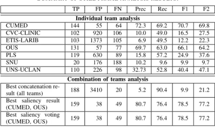
We present main still frame analysis results in both Fig. 6 (a) and in Table V. CUMED offers the best performance in all metrics evaluated, being the team which detected the most polyps (144) frames along with providing the lowest number of false alarms (55). The comparison between the performance of CNN-based approaches shows the importance of specific network configuration, as relevant differences in both number of detected polyp frames and false alarms can be observed - for instance, the number of detected polyp frames falls into a range between 131 (OUS) and 20 (SNU) -. Finally we can observe a performance gap between end-to-end learning and hybrid/hand-crafted methods, which provide less correct detections and significantly more false alarms. It has to be noted that as PLS provides four locations per image, the number of false alarms for this method is inherently higher than for other methods.
Considering full video analysis, the study shows superior performance by CNN-based methods -see Table VII and in
TABLE VI
SUMMARY OF STILL FRAME ANALYSIS RESULTS.
TP FP FN Prec Rec F1 F2
Individual team analysis
CUMED 144 55 64 72.3 69.2 70.7 69.8 CVC-CLINIC 102 920 106 10.0 49.0 16.5 27.5 ETIS-LARIB 103 1373 105 6.9 49.5 12.2 22.3 OUS 131 57 77 69.7 63.0 66.1 64.2 PLS 119 630 89 15.8 57.2 24.9 37.6 SNU 20 176 188 10.2 9.6 9.9 9.7 UNS-UCLAN 110 226 98 32.73 52.8 40.4 47.1 Combination of teams analysis
Best concatenation
re-sult (all teams) 188 3410 20 5.2 90.4 9.9 21.2 Best saliency result
(CUMED, OUS) 159 38 49 80.7 76.4 78.5 77.2 Best saliency voting
TABLE VII
SUMMARY OF THE MOST RELEVANT RESULTS REGARDING VIDEO SEQUENCE ANALYSIS.
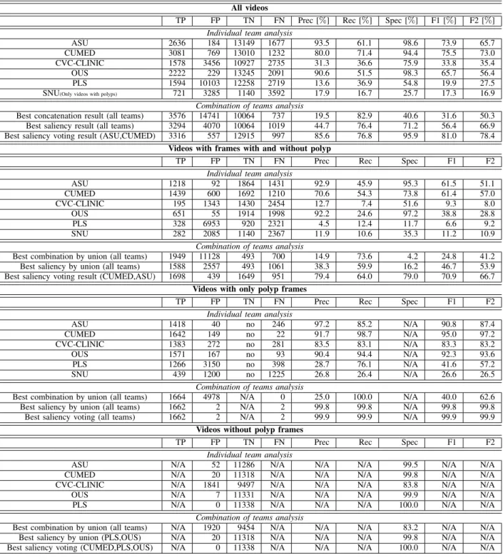
All videos
TP FP TN FN Prec [%] Rec [%] Spec [%] F1 [%] F2 [%] Individual team analysis
ASU 2636 184 13149 1677 93.5 61.1 98.6 73.9 65.7
CUMED 3081 769 13010 1232 80.0 71.4 94.4 75.5 73.0
CVC-CLINIC 1578 3456 10927 2735 31.3 36.6 75.9 33.8 35.4
OUS 2222 229 13245 2091 90.6 51.5 98.3 65.7 56.4
PLS 1594 10103 12258 2719 13.6 36.9 54.8 19.9 27.5
SNU(Only videos with polyps) 721 3285 1140 3592 17.9 16.7 25.7 17.3 16.9
Combination of teams analysis
Best concatenation result (all teams) 3576 14741 10064 737 19.5 82.9 40.6 31.6 50.3
Best saliency result (all teams) 3294 4070 10064 1019 44.7 76.4 71.2 56.4 66.9
Best saliency voting result (ASU,CUMED) 3316 557 12915 997 85.6 76.8 95.9 81.0 78.4
Videos with frames with and without polyp
TP FP TN FN Prec Rec Spec F1 F2
Individual team analysis
ASU 1218 92 1864 1431 92.9 45.9 95.3 61.5 51.1 CUMED 1439 600 1692 1210 70.6 54.3 73.8 61.4 57.0 CVC-CLINIC 195 1343 1430 2454 12.7 7.4 51.6 9.3 8.0 OUS 651 55 1914 1998 92.2 24.6 97.2 38.8 28.8 PLS 328 6953 920 2321 4.5 12.4 11.7 6.6 9.2 SNU 282 2085 1140 2367 11.9 10.6 35.3 11.2 10.9
Combination of teams analysis
Best combination by union (all teams) 1949 11128 493 700 14.9 73.6 4.2 24.8 41.2
Best saliency by union (all teams) 1588 2557 493 1061 38.3 59.9 16.2 46.7 53.9
Best saliency voting result (CUMED,ASU) 1698 439 1649 951 79.4 64.0 79.0 70.9 66.7
Videos with only polyp frames
TP FP TN FN Prec Rec Spec F1 F2
Individual team analysis
ASU 1418 40 no 246 97.2 85.2 N/A 90.8 87.4 CUMED 1642 149 no 22 91.7 98.7 N/A 95.0 97.2 CVC-CLINIC 1383 272 no 281 83.5 83.1 N/A 83.3 83.2 OUS 1571 167 no 93 90.4 94.4 N/A 92.3 93.6 PLS 1266 3150 no 398 28.7 76.1 N/A 41.6 57.2 SNU 439 1200 no 1225 26.8 26.4 N/A 26.6 26.5
Combination of teams analysis
Best combination by union (all teams) 1664 4978 N/A 0 25.0 100.0 N/A 40.0 62.6
Best saliency by union (all teams) 1662 2 N/A 2 99.8 99.8 N/A 99.8 99.8
Best saliency voting (all teams) 1662 2 N/A 2 99.9 99.9 N/A 99.9 99.9
Videos without polyp frames
TP FP TN FN Prec Rec Spec F1 F2
Individual team analysis
ASU N/A 52 11286 N/A N/A N/A 99.5 N/A N/A
CUMED N/A 20 11318 N/A N/A N/A 99.8 N/A N/A
CVC-CLINIC N/A 1841 9497 N/A N/A N/A 83.8 N/A N/A
OUS N/A 7 11331 N/A N/A N/A 99.9 N/A N/A
PLS N/A 0 11338 N/A N/A N/A 100.0 N/A N/A
Combination of teams analysis
Best combination by union (all teams) N/A 1920 9454 N/A N/A N/A 83.2 N/A N/A
Best saliency by union (PLS,OUS) N/A 20 11318 N/A N/A N/A 99.8 N/A N/A
Best saliency voting (CUMED,PLS,OUS) N/A 0 11338 N/A N/A N/A 100.0 N/A N/A
Fig. 6 (b)- , with CUMED being the method providing a higher number of polyp frames detected (3081). In this case, it has to be noted that CUMED does not outperform all other methods in all considered metrics, as ASU provides a better balance between true and false alarms (higher F1-score) at the cost of detecting less polyp frames (2636 vs. 3081).
We present in Table VII a complete breakdown of video analysis results, dividing them into 3 groups according to the degree of polyp presence in the sequences: 1) videos containing frames with and without polyps; 2) videos con-taining only frames with polyps, and 3) videos concon-taining
non-polyp frames. In all cases, results again show a superior performance of CUMED in terms of total number of polyp frames detected. Deepening the analysis, we observe a de-crease in the difference in performance observed in global analysis between hand-crafted methods (CVC-CLINIC) and CNN-based methods when videos with only polyp frames are analyzed. This can be related to those methods being designed to highlight polyp-like structures in the image (localization) but not for determining specific polyp presence. The analysis of sequences without polyp frames shows that PLS offers the best performance, which is possibly due to the presence of a
(a) (b)
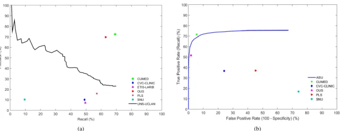
Fig. 6. Performance curves: (a) Precision-Recall curve for the analysis of the ETIS-LARIB database and (b) Receiver Operating Characteristic (ROC curves) for the analysis of the ASU-Mayo database. For the ROC curve, SNU operating point is calculated from the videos the team provided results for. Methods are represented with a line in cases where the confidence value has been provided for each detection, otherwise the operating point is used.
specific polyp presence module in this approach.
As mentioned in Section III-C, a statistical analysis is performed to account for differences in performance between methods. Results of the Saphiro-Wilk test over the F1 results for each video and method indicates a normal data distribution (p−value >0.05). Considering this, we perform a subsequent ANOVA analysis and multicomparison test to compare the different methods. The ANOVA test detects significant dif-ferences across F1 values (p−value= 5.4e−10), which are explored in the multicomparison test shown in Fig. 8. Results of this test show the superior performance of ASU, providing CUMED with a comparable performance different from the rest in a statistically significant way. CUMED and OUS also show performances comparable to each other. Finally CVC, PLS, and SNU also present comparable performances.
We present in Fig. 7 detection latency results. We can observe how there are only two teams (ASU and CUMED) which present latency scores for all the videos. We perform a statistical analysis to account for the differences between them. The result of the Saphiro-Wilk test indicates a non-normal data distribution (p−value < 0.05) and, consequently, the Kruskal-Wallis test is performed to account for statistically significant differences. In this case the test confirms the null hypothesis that both data samples come from the same distributionp−value= 0.76, which can be observed in Fig.8.
Fig. 7. Detection latency for polyp-containing videos.
Concerning the rest of the methods, we can observe that they do not detect the polyps in all the videos which is also a cause of the difference in performances shown in Table VII.
B. Additional validation experiments
1) Combination of methods: We have included in Table IV-A and in Table VII the best performance achieved after applying each of the proposed method combination strategies. The most important though logical conclusion extracted is that a combination of methods leads to better detection results. As expected, any combination of methods leads to an increase of the total number of detected polyps. This shows that different methods detect different polyps and that even those with lower performance can contribute positively to the overall detection. We can observe in Fig. 9 (d-f) that if we do not include all teams in the combination, the number of correct polyp frame detections could be affected. We can also observe in Fig. 9 (a-c) that the combination of the two best methods in
Fig. 8. Multicomparison test for the analysis of the F1 score in videos showing frames with and without polyps. Each method is represented as a horizontal line whose center is located in corresponding method’s mean F1 score and whose width corresponds to the variance calculated according anova1 fit model. The best ranked group is represented by a blue horizontal line, comparable methods are shown in grey, and methods that are different in a statistically significant way are shown in red.
(a) (b)
(c) (d)
(e) (f)
Fig. 9. Examples of the benefits of using a saliency-map-based approach. The first row shows the impact of combining the two best methods that surpass their individual performances: (a) original image; (b) saliency map with the position of detection points superimposed (best method, CUMED); (c) saliency map with the position of detection points superimposed (two best method, CUMED and OUS). The second row shows the positive impact of the worst performing method: (d) original image; (e) saliency map with the position of detection points superimposed (all method); (f) saliency map with the position of detection points superimposed (all method but SNU). The polyp contour is represented in blue. Each method is represented by a different color and shape.
each category surpasses the individual methods’ performance, which indicates the potential of saliency map methods to build up more reliable systems. It is clear that the combination by union strategy increases the total number of detected polyp frames at the cost of vastly increasing the number of false alarms and, consequently, other strategies should be explored to achieve a clinically useful system.
Considering this, we observe that the use of saliency maps leads to a better balance between correct and false alarms. Regarding the two saliency-map sub-strategies, the voting strategy leads to a slightly better performance for the case of still frame analysis, specifically observed in the reduction of FP. This can be explained as being due to those poorly performing methods providing outputs for almost all frames. Once their contribution is not considered as majority is not achieved for a particular frame, these false alarms vanish.
Taking into account these results, if we consider a potential combination of methods as the solution for polyp detection, we would propose saliency maps with a voting sub-strategy as the strategy that leads to a better compromise between correct detections and false alarms, though other potential combinations can be explored. For instance, we can think of
a system which also includes the specific detection modules that some approaches have presented here (PLS, SNU), with polyp localization within a given image being then obtained using CNN-based approaches (CUMED, OUS).
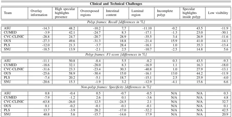
2) Impact of image challenges on individual methods’ performance: We present in Table VIII a summary of the results of the experiment assessing the impact of several image challenges on individual methods’ performance. With respect to polyp frames, the first conclusion to be extracted is that low visibility images and the presence of specular highlights within the polyp affect all methods in the same way. We interpret the impact of image quality as being both mucosa wall and its elements, such as polyps, better visually defined in good visibility images hence helping in polyp detection. We associate the positive impact of specular highlights inside the polyp to polyps appearing commonly as protruding elements in the scene and, as a consequence of this, specularities appear in their surface as their reflect light back to the camera [52].
There are some image challenges that generally seem to make polyp frames detection difficult such as the presence of overlay information and overexposed regions, with the latter being more prevalent in the explored images. The clear view of the luminal region also negatively affects detection capabil-ities, which we interpret as result of lumen presenting strong boundaries and contrast in comparison with the mucosa, which is a feature that polyps also exhibit. Surprisingly, the presence of intestinal content affects positively Recall and F1-score; this could be explained by the fact that this image challenge appears clearly different from polyps (weak contours, different color). Finally, the degree of completeness of the polyp seems to present a low impact on the performance of the methods, specially regarding F1-score.
Regarding non-polyp frames, we can observe that the pres-ence of overlay information and overexposed regions helps methods to discard frames without a polyp. Intestinal content leads to more false alarms, as does the presence of the luminal region and the presence of specular highlights; the three of them may falsely indicate the presence of a polyp, as the may also present contrast to mucosa or an indication of protrudness. We can also observe how methods tend to provide a higher number of false alarms for good quality images, which we interpret as a result of structures likely to be confused with polyps being better visually defined.
With respect to individual methods, we observe that those including boundary information (ASU, CVC-CLINIC and SNU) in their methodologies are specially damaged by the presence of structures with strong boundaries such as lumen or overlay information. End-to-end learning approaches are less affected in non-polyp frames analysis and they benefit from the presence of specular highlights in polyp frames.
3) Impact of polyp morphology on methods’ performance:
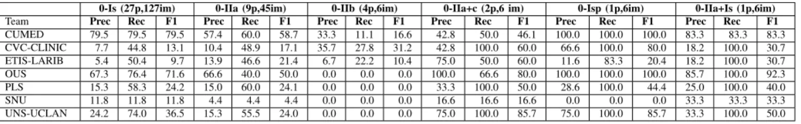
We present in Table X and in Table IX results of the study on the impact on polyp morphology on method’s performance. It has to be noted that we only provide results for the mor-phologies that appear in each particular database, as described in Section III. We can observe that for both still frames and video sequences analysis, methods’ performance do depend on polyp morphology. With respect to still frame analysis, we
TABLE VIII
IMPACT OF CLINICAL AND TECHNICAL CHALLENGES ON INDIVIDUAL METHODS’PERFORMANCE.
Clinical and Technical Challenges
Team Overlay information High specular highlights presence Overexposed regions Intestinal content Luminal region Incomplete polyp Specular highlights inside polyp Low visibility Polyp frames: Recall [differences in%]
ASU -14.3 48.2 -10.2 7,7 -11.10 -0.2 43.5 -11.9 CUMED -3.9 42.1 -24.7 8.3 -17.1 -1.3 23.0 -30.1 CVC-CLINIC -28.8 24.7 -20.7 28.9 -35.5 3.4 26.9 -11.6 OUS -27.3 49.6 -31.3 18.8 -21.4 15.9 41.0 -14.1 PLS -12.0 21.3 -3.7 28.4 -16.1 1.0 35.3 -13.4 SNU -18.5 13.9 -2.1 2.5 -10.7 -2.5 14.8 5.6
Polyp frames: F1-score [differences in%]
ASU -11.1 50.8 -8.4 5.5 -8.2 0.3 43.5 -9.3 CUMED -18.6 32.1 -28.0 8.3 -16.9 1.1 16.3 -18.0 CVC-CLINIC -31.6 23.3 -23.4 30.3 -40.8 1.0 27.9 -13.1 OUS -25.6 58.9 -30.4 15.0 -16.1 13.0 44.2 -11.9 PLS -7.4 20.2 -5.1 18.7 -15.1 2.5 25.9 -4.0 SNU -20.6 15.3 -1.9 3.2 -12.9 -4.1 15.6 6.6
Non-polyp frames: Specificity [differences in%]
ASU 0.8 -0.4 0.5 -0.7 -0.5 N/A N/A 0.3
CUMED -7.9 -1.2 2.6 0.1 -3.6 N/A N/A 4.8
CVC-CLINIC -63.8 -26.0 12.5 -24.5 2.1 N/A N/A 32.7
OUS 0.1 -0.2 -0.1 -0.1 -0.1 N/A N/A 0.1
PLS 13.7 -3.9 28.2 -17.0 -32.2 N/A N/A 42.5
SNU 40.8 5.6 -15.7 -14.6 17.9 N/A N/A 20.9
can observe that Recall scores are higher for sessile polyps (including sub-types 0-ISp and 0-IIa+Is) than for those less elevated (including flat) ones. We associate this to appearing sessile polyps more different to the mucosa and hence attract-ing the attention of the different methods. We can also observe how CVC-CLINIC and ETIS-LARIB , despite offering worse overall performance, are able to detect all kind of polyps though they obtain worse Precision scores.
Concerning video sequences, differences regarding degree of polyp elevation follow the same trend; in this case we can observe big differences in Recall for all methods but, in this case, Precision is not greatly affected but for the case of CVC-CLINIC, which is logical due to its big dependence on boundary presence to guide polyp detection; boundaries between mucosa and the polyp are less distinguishable for the case of slightly elevated polyps. Finally, this positive increase in Recall score associated to sessile polyps also has an impact in latency score; all teams achieve smaller latency scores for those videos containing polyps of this morphological type (videos 2, 6, 8 and 9) in Fig. 7.
TABLE IX
IMPACT OF POLYP MORPHOLOGY IN METHODS’PERFORMANCE: VIDEO SEQUENCE ANALYSIS. ONLY FRAMES CONTAINING A POLYP ARE
CONSIDERED FOR METRICS CALCULATION.
0-Is (4 polyps, 2212 images) 0-IIa (5 polyps, 2101 images) Prec Rec F1 Lat Prec Rec F1 Lat ASU 97.4 73.7 83.9 0.5 97.2 47.9 64.1 13.4 CUMED 92.1 86.8 89.4 0.0 77.3 55.3 64.4 16.8 CVC-CLINIC 81.9 62.5 70.9 0.3 19.3 9.3 12.5 46.7 OUS 90.9 77.6 83.7 0.0 92.1 24.1 38.2 18.7 PLS 24.6 62.6 35.3 3.5 10.2 9.9 10.1 46.0 SNU 26.6 23.3 24.9 79.0 15.9 9.7 12.1 42.4
4) Temporal coherence on method’s response: We present results of our temporal coherence study on Table XI(a). For both consecutive frame and within sequence detection stability, we can observe that results follow the same trend than the analysis of individual frames, being CUMED and ASU the teams which present a higher degree of temporal coherence, despite none of them including temporal information as part of their methodology. We can also observe how CUMED and ASU are able to correctly detect polyp frames in more than half of the polyp frames that each sequence contain, which can be associated to them being more capable to cope with polyp appearance variability within a same sequence.
5) Analysis of the direct output of the methods: We present mean and standard deviation values of CR in Table XI(b). As we can observe, CUMED achieves the higher mean CR value across all frames fromETIS-LARIB database, concentrating around half of the total energy of the image inside the polyp. It has to be noted that, in this case, differences between methods can be associated to several reasons. First of all, it is clear that methods detecting correctly more polyps will be prone to concentrate more energy inside them hence the superior performance of CUMED, which was the best performing team in still frame analysis. Second, we also have to consider how the actual output of the method looks like, as it can have an impact in the specific metric considered.
We observe in Fig. 10 how some methods do not provide probabilistic energy maps but binary masks approximating the polyp region. Due to these regions having pre-determined shapes, two problems may appear. First, it is highly unlikely that actual polyps fit those shapes, so that any pixel-wise metric value can be damaged by the shape choice. Second,
TABLE X
IMPACT OF POLYP MORPHOLOGY IN METHODS’PERFORMANCE: STILL FRAME ANALYSIS.
0-Is (27p,127im) 0-IIa (9p,45im) 0-IIb (4p,6im) 0-IIa+c (2p,6 im) 0-Isp (1p,6im) 0-IIa+Is (1p,6im)
Team Prec Rec F1 Prec Rec F1 Prec Rec F1 Prec Rec F1 Prec Rec F1 Prec Rec F1
CUMED 79.5 79.5 79.5 57.4 60.0 58.7 33.3 11.1 16.6 42.8 50.0 46.1 100.0 100.0 100.0 83.3 83.3 83.3 CVC-CLINIC 7.7 44.8 13.1 10.4 48.9 17.1 35.7 27.8 31.2 42.8 100.0 60.0 66.6 100.0 80.0 18.2 100.0 30.7 ETIS-LARIB 5.4 50.4 9.7 13.9 46.6 21.4 6.7 22.2 10.4 75.0 50.0 60.0 11.6 83.3 20.4 18.2 100.0 30.7 OUS 67.3 76.4 71.6 66.6 40.0 50.0 0.0 0.0 0.0 100.0 66.6 80.0 100.0 100.0 100.0 85.7 100.0 92.3 PLS 15.3 58.3 24.2 15.0 60.0 24.1 0.0 0.0 0.0 33.3 100.0 50.0 28.6 100.0 44.4 25.0 100.0 40.0 SNU 11.8 11.8 11.8 4.4 4.4 4.4 0.0 0.0 0.0 16.6 16.6 16.6 0.0 0.0 0.0 33.3 33.3 33.3 UNS-UCLAN 24.2 74.0 36.5 15.3 55.5 24.0 0.0 0.0 0.0 75.0 100.0 85.7 75.0 100.0 85.7 33.3 100.0 50.0 (a) (b) (c) (d) (e) (f) (g) (h)
Fig. 10. Comparison of energy maps provided by each method: (a) original image (b) CUMED (c) CVC-CLINIC (d) PLS (e) UNS-UCLAN (f) ETIS-LARIB (g) OUS,s and (h) SNU. In each of the images, a green line represents the reference polyp mask.
if methods’ evaluation is based on the calculation of detection scores from single-position values and this position is calcu-lated as the centroid of the pre-determined shape in case of large regions partially covering the polyp, it may happen that the detection position falls outside the polyp when in fact part of the polyp region was covered by method’s output.
Consequently, we think it is not fair to include those meth-ods (ETIS-LARIB, OUS and SNU) in a CR-based comparison. We did statistically compare the different energy map-based methods. Preliminary results shown in Fig. 11 indicate again a superior performance of CUMED over the rest. Regarding the statistical significance of the differences, the Saphiro-Wilk test over CR values indicates a normal distribution of data. Therefore ANOVA and multicomparison tests are performed to study potential differences across methods. The ANOVA test detects significant differences across CR values (p−value = 2.51e−61), which are explored in the
multi-comparison test shown in Fig. 11. CUMED’s performance is statistically different from the rest of the approaches, which present comparable performances between them.
TABLE XI
TEMPORAL COHERENCE ANDCONCENTRATION RATIO RESULTS. FOR EACH METHOD,MEAN AND STANDARD DEVIATION VALUES OF
CORRESPONDING METRIC ARE PROVIDED. (a) Temporal Coherence
Method Consecutive frames Within sequence ASU 54.8±21.4 61.2±21.9 CUMED 63.7±23.9 67.7±23.2 CVC-CLINIC 34.1±37.6 30.3±37.0 OUS 48.7±30.8 47.2±34.1 PLS 27.4±26.1 31.7±30.4 SNU 10.2±06.3 11.7±11.7 (b) Concentration Ratio Method Value CUMED 48.5±26.7 CVC-CLINIC 17.9±24.1 PLS 11.9±14.4 UNS-UCLAN 18.7±18.8 V. DISCUSSION
A. Impact of the methodology used on method’s performance
The main result of this comparative study is that methods including some degree of machine learning outperform classic hand-crafted methods, specially regarding specificity scores in non-polyp videos. This correlates with the trend actually observed on computer vision research; methods traditionally were hybrid, using hand-crafted features and machine learning to classify a given input image according to the specific problem to solve. There is an extensive amount of hand-crafted features defined within the computer vision community, cover-ing from general ones such as HOG or SIFT features to others more domain-specific, such as the ones presented by CVC-Clinic team. Designing hand-crafted features to solve specific problems can be complicated and highly time consuming, as well as limiting the widespread use of a new developed technology.
CNNs allow to learn jointly problem-specific features and the classifier to differentiate among classes. Their great power comes from the ability of learning problem-specific features in an increasing depth of complexity and abstraction. As it has been shown in this paper, we can observe a supe-rior performance of CNN-based approaches over hand-crafted methods. We can also observe differences in performance between CNN-based methods which shows how obtaining good performance of these networks depends strongly on defining the proper architecture and having quality data to feed the network. Regarding the design of the network, there are several details to take into account which go from pure
Fig. 11. The multicomparison test for the analysis of the CR score in the ETIS-LARIB database. Each method is represented as a horizontal line centered in corresponding method’s mean CR score and whose width corresponds to the variance calculated according anova1 fit model. The best ranked group is represented by a blue line, comparable methods are shown in grey, and statistically significant different methods are shown in red.