Adaptive Parameter-free Learning from Evolving Data Streams
Albert Bifet
Ricard Gavald`a
Universitat Polit`ecnica de Catalunya
{
abifet, gavalda
}
@lsi.up.edu
Abstract
We propose and illustrate a method for developing algorithms that can adaptively learn from data streams that change over time. As an example, we take Hoeffding Tree, an incremental decision tree inducer for data streams, and use as a basis it to build two new methods that can deal with distribution and concept drift: a sliding window-based algorithm, Hoeffding Window Tree, and an adaptive method, Hoeffding Adaptive Tree. Our methods are based on using change detectors and estimator modules at the right places; we choose implementations with theoretical guarantees in order to extend such guarantees to the resulting adaptive learning algorithm. A main advantage of our methods is that they require no guess about how fast or how often the stream will change; other methods typically have several user-defined parameters to this effect.
In our experiments, the new methods never do worse, and in some cases do much better, than CVFDT, a well-known method for tree induction on data streams with drift.
1 Introduction
Data streams pose several challenges on data mining algo-rithm design. Limited use of resources (time and memory) is one. The necessity of dealing with data whose nature or distribution changes over time is another fundamental one. Dealing with time-changing data requires in turn strategies for detecting and quantifying change, forgetting stale exam-ples, and for model revision. Fairly generic strategies ex-ist for detecting change and deciding when examples are no longer relevant. Model revision strategies, on the other hand, are in most cases method-specific.
Most strategies for dealing with time change contain hardwired constants, or else require input parameters, con-cerning the expected speed or frequency of the change; some examples area prioridefinitions of sliding window lengths, values of decay or forgetting parameters, explicit bounds on maximum drift, etc. These choices represent preconceptions on how fast or how often the data are going to evolve and, of course, they may be completely wrong. Even more, no fixed choice may be right, since the stream may experience any combination of abrupt changes, gradual ones, and long stationary periods. More in general, an approach based on fixed parameters will be caught in the following tradeoff: the user would like to use large parameters to have more accu-rate statistics (hence, more precision) during periods of sta-bility, but at the same time use small parameters to be able to quickly react to changes, when they occur.
Many ad-hoc methods have been used to deal with drift,
often tied to particular algorithms. In this paper, we propose a more general approach based on using two primitive design elements: change detectors and estimators. The idea is to encapsulate all the statistical calculations having to do with detecting change and keeping updated statistics from a stream an abstract data type that can then be used to replace, in a black-box way, the counters and accumulators that typically all machine learning and data mining algorithms use to make their decisions, including when change has occurred.
We believe that, compared to any previous approaches, our approach better isolates different concerns when design-ing new data mindesign-ing algorithms, therefore reducdesign-ing design time, increasing modularity, and facilitating analysis. Fur-thermore, since we crisply identify the nuclear problem in dealing with drift, and use a well-optimized algorithmic so-lution to tackle it, the resulting algorithms more accurate, adaptive, and time- and memory-efficient than other ad-hoc approaches. We have given evidence for this superiority in [3, 2, 4] and we demonstrate this idea again here.
We apply this idea to give two decision tree learning algorithms that can cope with concept and distribution drift on data streams: Hoeffding Window Trees in Section 4 and Hoeffding Adaptive Trees in Section 5. Decision trees are among the most common and well-studied classifier models. Classical methods such as C4.5 are not apt for data streams, as they assume all training data are available simultaneously in main memory, allowing for an unbounded number of passes, and certainly do not deal with data that changes over time. In the data stream context, a reference work on learning decision trees is the Hoeffding Tree or Very Fast Decision Tree method (VFDT) for fast, incremental learning [7]. The methods we propose are based on VFDT, enriched with the change detection and estimation building blocks mentioned above.
We try several such building blocks, although the best suited for our purposes is the ADWIN algorithm [3], de-scribed in Section 4.1.1. This algorithm is parameter-free in that it automatically and continuously detects the rate of change in the data streams rather than using apriori guesses, thus allowing the client algorithm to react adaptively to the data stream it is processing. Additionally, ADWIN has
rig-orous guarantees of performance (a theorem). We show that these guarantees can be transferred to decision tree learners as follows: if a change is followed by a long enough stable period, the classification error of the learner will tend, and the same rate, to the error rate of VFDT.
We test on Section 6 our methods with synthetic datasets, using the SEA concepts, introduced in [22] and a rotating hyperplane as described in [13], and two sets from the UCI repository, Adult and Poker-Hand. We compare our methods among themselves but also with CVFDT, another concept-adapting variant of VFDT proposed by Domingos, Spencer, and Hulten [13]. A one-line conclusion of our ex-periments would be that, because of its self-adapting prop-erty, we can present datasets where our algorithm performs much better than CVFDT and we never do much worse. Some comparison of time and memory usage of our meth-ods and CVFDT is included.
2 A Methodology for Adaptive Stream Mining
The starting point of our work is the following observation: In the data stream mining literature, most algorithms incor-porate one or more of the following ingredients: windows to remember recent examples; methods for detecting distribu-tion change in the input; and methods for keeping updated estimations for some statistics of the input. We see them as the basis for solving the three central problems of
• what to remember or forget, • when to do the model upgrade, and • how to do the model upgrade.
Our claim is that by basing mining algorithms on well-designed, well-encapsulated modules for these tasks, one can often get more generic and more efficient solutions than by using ad-hoc techniques as required. Similarly, we will argue that our methods for inducing decision trees are simpler to describe, adapt better to the data, perform better or much better, and use less memory than the ad-hoc designed CVFDT algorithm, even though they are all derived from the same VFDT mining algorithm.
A similar approach was taken, for example, in [4] to give simple adaptive closed-tree mining adaptive algorithms. Us-ing a general methodology to identify closed patterns based in Galois Lattice Theory, three closed tree mining algo-rithms were developed: an incremental one INCTREENAT, a sliding-window based one, WINTREENAT, and finally one that mines closed trees adaptively from data streams, ADA -TREENAT.
2.1 Time Change Detectors and Predictors To choose a change detector or an estimator, we will review briefly all the different types of change detectors and estimators, in order to
-xt Estimator - -Alarm Change Detector -Estimation Memory -6 6 ?
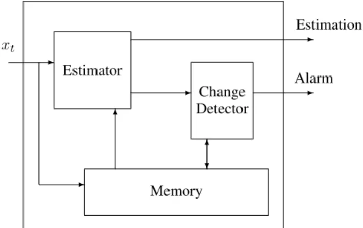
Figure 1: Change Detector and Estimator System
justify the election of one of them for our algorithms. Most approaches for predicting and detecting change in streams of data can be discussed as systems consisting of three modules: a Memory module, an Estimator Module, and a Change Detector or Alarm Generator module. These three modules interact as shown in Figure 1, which is analogous to Figure 8 in [21].
In general, the input to this algorithm is a sequence x1, x2, . . . , xt, . . . of data items whose distribution varies
over time in an unknown way. The outputs of the algorithm are, at each time step
• an estimation of some important parameters of the input distribution, and
• a signal alarm indicating that distribution change has recently occurred.
We consider a specific, but very frequent case, of this setting: that in which all thextare real values. The desired
estimation in the sequence ofxiis usually the expected value
of the currentxt, and less often another distribution statistics
such as the variance. The only assumption on the distribution is that eachxtis drawn independently from each other. Note
therefore that we deal with one-dimensional items. While the data streams often consist of structured items, most mining algorithms are not interested in the items themselves, but on a bunch of real-valued (sufficient) statistics derived from the items; we thus imagine our input data stream as decomposed into possibly many concurrent data streams of real values, which will be combined by the mining algorithm somehow.
Memory is the component where the algorithm stores the sample data or summary that considers relevant at current time, that is, its description of the current data distribution.
The Estimator component is an algorithm that estimates the desired statistics on the input data, which may change over time. The algorithm may or may not use the data contained in the Memory. The simplest Estimator algorithm for the expected is thelinear estimator,which simply returns
the average of the data items contained in the Memory. Other examples of efficient estimators are Auto-Regressive, Auto Regressive Moving Average, and Kalman filters.
The change detector component outputs an alarm signal when it detects change in the input data distribution. It uses the output of the Estimator, and may or may not in addition use the contents of Memory.
We classify these predictors in four classes, depending on whether Change Detector and Memory modules exist:
• Type I: Estimator only. The simplest one is modelled by
ˆ
xk= (1−α)ˆxk−1+α·xk.
The linear estimator corresponds to using α = 1/N whereN is the width of a virtual window containing the last N elements we want to consider. Otherwise, we can give more weight to the last elements with an appropriate constant value ofα. The Kalman filter tries to optimize the estimation using a non-constantα(the Kvalue) which varies at each discrete time interval. • Type II: Estimator with Change Detector. An
exam-ple is the Kalman Filter together with a CUSUM test change detector algorithm, see for example [15]. • Type III: Estimator with Memory. We add Memory to
improve the results of the Estimator. For example, one can build an Adaptive Kalman Filter that uses the data in Memory to compute adequate values for process and measure variances.
• Type IV: Estimator with Memory and Change Detector. This is the most complete type. Two examples of this type, from the literature, are:
– A Kalman filter with a CUSUM test and fixed-length window memory, as proposed in [21]. Only the Kalman filter has access to the memory. – A linear Estimator over fixed-length windows
that flushes when change is detected [17], and a change detector that compares the running win-dows with a reference window.
3 Incremental Decision Trees: Hoeffding Trees
Decision trees are classifier algorithms [5, 20]. Each internal node of a treeDTcontains a test on an attribute, each branch from a node corresponds to a possible outcome of the test, and each leaf contains a class prediction. The label y = DT(x)for an examplexis obtained by passing the example down from the root to a leaf, testing the appropriate attribute at each node and following the branch corresponding to the attribute’s value in the example. Extended models where the nodes contain more complex tests and leaves contain more complex classification rules are also possible.
A decision tree is learned top-down by recursively re-placing leaves by test nodes, starting at the root. The at-tribute to test at a node is chosen by comparing all the avail-able attributes and choosing the best one according to some heuristic measure.
Classical decision tree learners such as ID3, C4.5 [20], and CART [5] assume that all training examples can be stored simultaneously in main memory, and are thus severely limited in the number of examples they can learn from. In particular, they are not applicable to data streams, where potentially there is no bound on number of examples and these arrive sequentially.
Domingos and Hulten [7] developed Hoeffding trees, an incremental, anytime decision tree induction algorithm that is capable of learning from massive data streams, assuming that the distribution generating examples does not change over time.
Hoeffding trees exploit the fact that a small sample can often be enough to choose an optimal splitting attribute. This idea is supported mathematically by the Hoeffding bound, which quantifies the number of observations (in our case, examples) needed to estimate some statistics within a prescribed precision (in our case, the goodness of an attribute). More precisely, the Hoeffding bound states that with probability1−δ, the true mean of a random variable of rangeRwill not differ from the estimated mean after n independent observations by more than:
= r
R2ln(1/δ)
2n .
A theoretically appealing feature of Hoeffding Trees not shared by other incremental decision tree learners is that it has sound guarantees of performance. Using the Hoeffding bound one can show that its output is asymptotically nearly identical to that of a non-incremental learner using infinitely many examples. Theintensional disagreement∆i between
two decision treesDT1 andDT2is the probability that the
path of an example through DT1 will differ from its path
throughDT2.
THEOREM3.1. IfHTδ is the tree produced by the
Hoeffd-ing tree algorithm with desired probability δgiven infinite examples,DTis the asymptotic batch tree, andpis the leaf probability, thenE[∆i(HTδ, DT)]≤δ/p.
VFDT (Very Fast Decision Trees) is the implementation of Hoeffding trees, with a few heuristics added, described in [7]; we basically identify both in this paper. The pseudo-code of VFDT is shown in Figure 2. Counts nijk are the
sufficient statistics needed to choose splitting attributes, in particular the information gain function Gimplemented in VFDT. Function(δ, . . .)in line 4 is given by the Hoeffding bound and guarantees that whenever bestand2nd best at-tributes satisfy this condition, we can confidently conclude
VFDT(Stream, δ)
1 Let HT be a tree with a single leaf(root) 2 Init countsnijkat root
3 foreach example(x, y)in Stream 4 doVFDTGROW((x, y), HT, δ) VFDTGROW((x, y), HT, δ)
1 Sort(x, y)to leaflusingHT 2 Update countsnijkat leafl
3 ComputeGfor each attribute from countsni,j,k
4 ifG(Best Attr.)−G(2nd best)> (δ, . . .) 5 then
6 Split leaflon best attribute 7 foreach branch
8 doInitialize new leaf counts atl
Figure 2: The VFDT algorithm
thatbestindeed has maximal gain. The sequence of exam-ples S may be infinite, in which case the procedure never terminates, and at any point in time a parallel procedure can use the current tree to make class predictions.
4 Decision Trees on Sliding Windows
We propose a general method for building incrementally a decision tree based on a keeping sliding window of the last instances on the stream. To specify one such method, we specify how to:
• place one or more change detectors at every node that will raise a hand whenever something worth attention happens at the node
• create, manage, switch and delete alternate trees • maintain estimators of only relevant statistics at the
nodes of the current sliding window
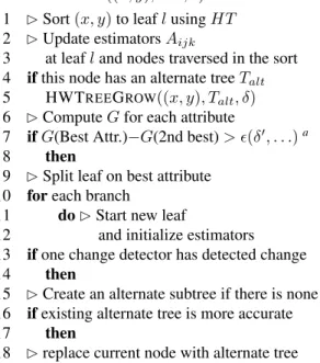
We call Hoeffding Window Tree any decision tree that uses Hoeffding bounds, maintains a sliding win-dow of instances, and that can be included in this gen-eral framework. Figure 3 shows the pseudo-code of HOEFFDINGWINDOWTREE.
4.1 HWT-ADWIN : Hoeffding Window Tree using ADWIN Recently, we proposed an algorithm termed ADWIN [3] (for Adaptive Windowing) that is an estimator with memory and change detector of type IV. We use it to design HWT-ADWIN, a new Hoeffding Window Tree that usesADWIN as a change detector. The main advantage of using a change detector asADWIN is that as it has
theoreti-HOEFFDINGWINDOWTREE(Stream, δ)
1 Let HT be a tree with a single leaf(root) 2 Init estimatorsAijkat root
3 foreach example(x, y)in Stream 4 doHWTREEGROW((x, y), HT, δ) HWTREEGROW((x, y), HT, δ)
1 Sort(x, y)to leaflusingHT 2 Update estimatorsAijk
3 at leafland nodes traversed in the sort 4 ifthis node has an alternate treeTalt
5 HWTREEGROW((x, y), Talt, δ)
6 ComputeGfor each attribute
7 ifG(Best Attr.)−G(2nd best)> (δ0, . . .)a
8 then
9 Split leaf on best attribute 10 foreach branch
11 doStart new leaf
12 and initialize estimators 13 ifone change detector has detected change 14 then
15 Create an alternate subtree if there is none 16 ifexisting alternate tree is more accurate 17 then
18 replace current node with alternate tree
aHereδ0should be theBonferroni correctionofδto account for the fact that many tests are performed and we want all of them to be simultaneously correct with probability1−δ. It is enough e.g. to divideδby the number of tests performed so far. The need for this correction is also acknowledged in [7], although in experiments the more convenient option of using a lowerδwas taken. We have followed the same option in our experiments for fair comparison.
cal guarantees we can extend this guarantees to the learning algorithms.
4.1.1 TheADWIN algorithm ADWIN is a change detec-tor and estimadetec-tor that solves in a well-specified way the prob-lem of tracking the average of a stream of bits or real-valued numbers. ADWIN keeps a variable-length window of re-cently seen items, with the property that the window has the maximal length statistically consistent with the hypothesis “there has been no change in the average value inside the window”.
The idea of ADWIN method is simple: whenever two “large enough” subwindows ofW exhibit “distinct enough” averages, one can conclude that the corresponding expected values are different, and the older portion of the window is dropped. The meaning of “large enough” and “distinct enough” can be made precise again by using the Hoeffding bound. The test eventually boils down to whether the average of the two subwindows is larger than a variable value cut
computed as follows m := 2 1/|W0|+ 1/|W1| cut := r 1 2m ·ln 4|W| δ . wheremis the harmonic mean of|W0|and|W1|.
The main technical result in [3] about the performance of ADWIN is the following theorem, that provides bounds on the rate of false positives and false negatives forADWIN: THEOREM4.1. With cut defined as above, at every time
step we have:
1. (False positive rate bound).Ifµthas remained constant
within W, the probability that ADWIN shrinks the window at this step is at mostδ.
2. (False negative rate bound). Suppose that for some partition ofW in two partsW0W1(whereW1contains
the most recent items) we have|µW0−µW1|> 2cut.
Then with probability1−δADWIN shrinksWtoW1,
or shorter.
This theorem justifies us in usingADWIN in two ways: • as achange detector, sinceADWIN shrinks its window
if and only if there has been a significant change in recent times (with high probability)
• as anestimatorfor the current average of the sequence it is reading since, with high probability, older parts of the window with a significantly different average are automatically dropped.
ADWIN is parameter- and assumption-free in the sense that it automatically detects and adapts to the current rate of change. Its only parameter is a confidence boundδ, indicat-ing how confident we want to be in the algorithm’s output, inherent to all algorithms dealing with random processes.
Also important for our purposes, ADWIN does not maintain the window explicitly, but compresses it using a variant of the exponential histogram technique in [6]. This means that it keeps a window of length W using only O(logW)memory andO(logW)processing time per item, rather than theO(W)one expects from a na¨ıve implementa-tion.
4.1.2 Example of performance Guarantee Let HWT∗ADWIN be a variation of HWT-ADWIN with the following condition: every time a node decides to create an alternate tree, an alternate tree is also started at the root. In this section we show an example of performance guarantee about the error rate of HWT∗ADWIN. Informally speaking, it states that after a change followed by a stable period, HWT∗ADWIN’s error rate will decrease at the same rate as that of VFDT, after a transient period that depends only on the magnitude of the change.
We consider the following scenario: Let C andD be arbitrary concepts, that can differ both in example distribu-tion and label assignments. Suppose the input data sequence S is generated according to concept C up to time t0, that
it abruptly changes to concept D at timet0+ 1, and
re-mains stable after that. Let HWT∗ADWIN be run on se-quence S, ande1 be error(HWT∗ADWIN,S,t0), ande2 be
error(HWT∗ADWIN,S,t0+ 1), so thate2−e1measures how
much worse the error of HWT∗ADWIN has become after the concept change.
Here error(HWT∗ADWIN,S,t) denotes the classification error of the tree kept by HWT∗ADWIN at time t on S. Similarly, error(VFDT,D,t) denotes the expected error rate of the tree kept by VFDT after being fed with t random examples coming from conceptD.
THEOREM4.2. LetS,t0,e1, ande2be as described above,
and supposet0 is sufficiently large w.r.t. e2−e1. Then for
every timet > t0, we have
error(HWT∗ADWIN, S, t)≤min{e2, eV F DT}
with probability at least1−δ, where
• eV F DT = error(V F DT, D, t−t0−g(e2−e1)) +
O(√1
t−t0)
• g(e2−e1) = 8/(e2−e1)2ln(4t0/δ)
The following corollary is a direct consequence, since O(1/√t−t0)tends to0astgrows.
COROLLARY4.1. If error(VFDT,D,t) tends to some quan-tity ≤ e2 as t tends to infinity, then error(HWT∗ADWIN
,S,t) tends totoo.
Proof. Note: The proof is only sketched in this version. We know by the ADWIN False negative rate bound that with probability1−δ, theADWIN instance monitoring the error rate at the root shrinks at timet0+nif
|e2−e1|>2cut=
p
2/mln(4(t−t0)/δ)
wheremis the harmonic mean of the lengths of the subwin-dows corresponding to data before and after the change. This condition is equivalent to
m >4/(e1−e2)2ln(4(t−t0)/δ)
Ift0is sufficiently large w.r.t. the quantity on the right hand
side, one can show thatmis, say, less thann/2by definition of the harmonic mean. Then some calculations show that for n ≥g(e2−e1)the condition is fulfilled, and therefore by
timet0+nADWIN will detect change.
After that, HWT∗ADWIN will start an alternative tree at the root. This tree will from then on grow as in VFDT, because HWT∗ADWIN behaves as VFDT when there is no concept change. While it does not switch to the alternate tree, the error will remain ate2. If at any timet0+g(e1−
e2) +nthe error of the alternate tree is sufficiently below
e2, with probability1−δthe twoADWIN instances at the
root will signal this fact, and HWT∗ADWIN will switch to the alternate tree, and hence the tree will behave as the one built by VFDT withtexamples. It can be shown, again by using the False Negative Bound onADWIN , that the switch will occur when the VFDT error goes belowe2−O(1/
√ n), and the theorem follows after some calculation.
4.2 CVFDT As an extension of VFDT to deal with con-cept change Hulten, Spencer, and Domingos presented Concept-adapting Very Fast Decision Trees CVFDT [13] al-gorithm. We review it here briefly and compare it to our method.
CVFDT works by keeping its model consistent with re-spect to a sliding window of data from the data stream, and creating and replacing alternate decision subtrees when it de-tects that the distribution of data is changing at a node. When new data arrives, CVFDT updates the sufficient statistics at its nodes by incrementing the countsnijk corresponding to
the new examples and decrementing the countsnijk
corre-sponding to the oldest example in the window, which is ef-fectively forgotten. CVFDT is a Hoeffding Window Tree as it is included in the general method previously presented.
Two external differences among CVFDT and our method is that CVFDT has no theoretical guarantees (as far as we know), and that it uses a number of parameters, with default values that can be changed by the user - but which
are fixed for a given execution. Besides the example window length, it needs:
1. T0: after eachT0 examples, CVFDT traverses all the
decision tree, and checks at each node if the splitting attribute is still the best. If there is a better splitting attribute, it starts growing an alternate tree rooted at this node, and it splits on the currently best attribute according to the statistics in the node.
2. T1: after an alternate tree is created, the followingT1
examples are used to build the alternate tree.
3. T2: after the arrival ofT1 examples, the followingT2
examples are used to test the accuracy of the alternate tree. If the alternate tree is more accurate than the current one, CVDFT replaces it with this alternate tree (we say that the alternate tree is promoted).
The default values are T0 = 10,000, T1 = 9,000,
and T2 = 1,000. One can interpret these figures as the
preconception that often about the last50,000examples are likely to be relevant, and that change is not likely to occur faster than every 10,000 examples. These preconceptions may or may not be right for a given data source.
The main internal differences of HWT-ADWIN respect CVFDT are:
• The alternates trees are created as soon as change is detected, without having to wait that a fixed number of examples arrives after the change. Furthermore, the more abrupt the change is, the faster a new alternate tree will be created.
• HWT-ADWIN replaces the old trees by the new alter-nates trees as soon as there is evidence that they are more accurate, rather than having to wait for another fixed number of examples.
These two effects can be summarized saying that HWT-ADWIN adapts to the scale of time change in the data, rather than having to rely on thea prioriguesses by the user. 5 Hoeffding Adaptive Trees
In this section we present Hoeffding Adaptive Tree as a new method that evolving from Hoeffding Window Tree, adaptively learn from data streams that change over time without needing a fixed size of sliding window. The optimal size of the sliding window is a very difficult parameter to guess for users, since it depends on the rate of change of the distribution of the dataset.
In order to avoid to choose a size parameter, we propose a new method for managing statistics at the nodes. The general idea is simple: we place instances of estimators of frequency statistics at every node, that is, replacing eachnijk
counters in the Hoeffding Window Tree with an instance Aijkof an estimator.
More precisely, we present three variants of aHoeffding Adaptive Treeor HAT, depending on the estimator used:
• HAT-INC: it uses a linear incremental estimator • HAT-EWMA: it uses an Exponential Weight Moving
Average (EWMA)
• HAT-ADWIN : it uses an ADWIN estimator. As the ADWIN instances are also change detectors, they will give an alarm when a change in the attribute-class statistics at that node is detected, which indicates also a possible concept change.
The main advantages of this new method over a Hoeffd-ing Window Tree are:
• All relevant statistics from the examples are kept in the nodes. There is no need of an optimal size of sliding window for all nodes. Each node can decide which of the last instances are currently relevant for it. There is no need for an additional window to store current examples. For medium window sizes, this factor substantially reduces our memory consumption with respect to a Hoeffding Window Tree.
• A Hoeffding Window Tree, as CVFDT for example, stores only a bounded part of the window in main memory. The rest (most of it, for large window sizes) is stored in disk. For example, CVFDT has one parameter that indicates the amount of main memory used to store the window (default is 10,000). Hoeffding Adaptive Trees keeps all its data in main memory.
5.1 Example of performance Guarantee In this subsec-tion we show a performance guarantee on the error rate of HAT-ADWIN on a simple situation. Roughly speaking, it states that after a distribution and concept change in the data stream, followed by a stable period, HAT-ADWIN will start, in reasonable time, growing a tree identical to the one that VFDT would grow if starting afresh from the new stable dis-tribution. Statements for more complex scenarios are possi-ble, including some with slow, gradual, changes, but require more space than available here.
THEOREM5.1. Let D0 and D1 be two distributions on
labelled examples. Let S be a data stream that contains examples followingD0for a timeT, then suddenly changes
to usingD1. Lettbe the time that until VFDT running on a
(stable) stream with distributionD1takes to perform a split
at the node. Assume also that VFDT onD0andD1builds
trees that differ on the attribute tested at the root. Then with probability at least1−δ:
• By time t0 = T +c ·V2 · tlog(tV), HAT-ADWIN
will create at the root an alternate tree labelled with the same attribute as VFDT(D1). Herec ≤ 20is an
absolute constant, and V the number of values of the attributes.1
• this alternate tree will evolve from then on identically as does that of VFDT(D1), and will eventually be
promoted to be the current tree if and only if its error onD1is smaller than that of the tree built by timeT.
If the two trees do not differ at the roots, the correspond-ing statement can be made for a pair of deeper nodes. LEMMA5.1. In the situation above, at every timet+T > T, with probability1−δwe have at every node and for every counter (instance ofADWIN)Ai,j,k
|Ai,j,k−Pi,j,k| ≤
s
ln(1/δ0)T
t(t+T)
where Pi,j,k is the probability that an example arriving at
the node has valuejin itsith attribute and classk.
Observe that for fixedδ0andTthis bound tends to0as
tgrows.
To prove the theorem, use this lemma to prove high-confidence bounds on the estimation of G(a) for all at-tributes at the root, and show that the attributebestchosen by VFDT onD1will also have maximalG(best)at some point,
so it will be placed at the root of an alternate tree. Since this new alternate tree will be grown exclusively with fresh ex-amples fromD1, it will evolve as a tree grown by VFDT on
D1.
5.2 Memory Complexity Analysis Let us compare the memory complexity Hoeffding Adaptive Trees and Hoeffd-ing Window Trees. We take CVFDT as an example of Ho-effding Window Tree. Denote with
• E : size of an example • A : number of attributes
• V : maximum number of values for an attribute • C : number of classes
• T : number of nodes
A Hoeffding Window Tree as CVFDT uses memory O(W E +T AV C), because it uses a window W with E examples, and each node in the tree usesAV Ccounters. A
1This value of t0 is a very large overestimate, as indicated by our experiments. We are working on an improved analysis, and hope to be able to reducet0toT+c·t, forc <4.
Hoeffding Adaptive Tree does not need to store a window of examples, but uses instead memoryO(logW)at each node as it uses anADWIN as a change detector, so its memory re-quirement is O(T AV C+TlogW). For medium-size W, the O(W E)in CVFDT can often dominate. HAT-ADWIN has a complexity ofO(T AV ClogW).
6 Experimental evaluation
We tested Hoeffding Adaptive Trees using synthetic and real datasets. In the experiments with synthetic datasets, we use the SEA Concepts [22] and a changing concept dataset based on a rotating hyperplane explained in [13]. In the experiments with real datasets we use two UCI datasets [1] Adult and Poker-Hand from the UCI repository of machine learning databases. In all experiments, we use the values δ = 10−4,T0 = 20,000, T1 = 9,000, andT2 = 1,000,
following the original CVFDT experiments [13].
In all tables, the result for the best classifier for a given experiment is marked in boldface, and the best choice for CVFDT window length is shown initalics.
We included an improvement over CVFDT (which could be made on the original CVFDT as well). If the two best attributes at a node happen to have exactly the same gain, the tie may be never resolved and split does not occur. In our experiments this was often the case, so we added an additional split rule: whenG(best)exceeds by three times the current value of(δ, . . .), a split is forced anyway.
We have tested the three versions of Hoeffding Adaptive Tree, HAT-INC, HAT-EWMA(α=.01), HAT-ADWIN, each with and without the addition of Na¨ıve Bayes (NB) classi-fiers at the leaves. As a general comment on the results, the use of NB classifiers does not always improve the results, although it does make a good difference in some cases; this was observed in [11], where a more detailed analysis can be found.
First, we experiment using the SEA concepts, a dataset with abrupt concept drift, first introduced in [22]. This artificial dataset is generated using three attributes, where only the two first attributes are relevant. All three attributes have values between 0 and 10. We generate 400,000 random samples. We divide all the points in blocks with different concepts. In each block, we classify using f1+f2 ≤ θ,
wheref1andf2 represent the first two attributes andθis a
threshold value.We use threshold values 9, 8, 7 and 9.5 for the data blocks. We inserted about 10% class noise into each block of data.
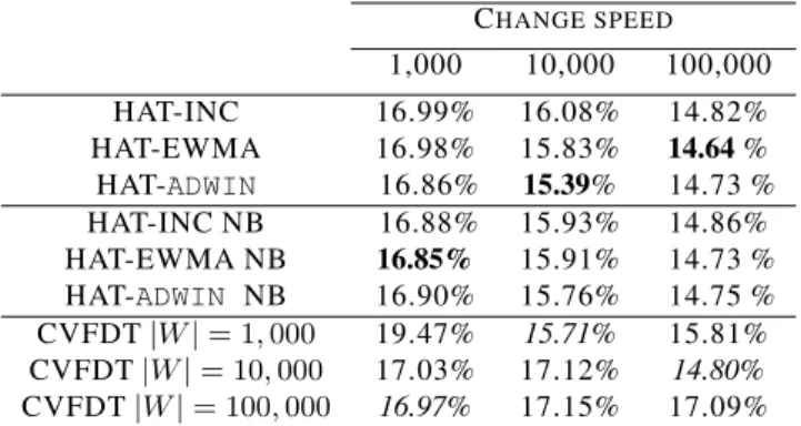
We test our methods using discrete and continuous attributes. The on-line errors results for discrete attributes are shown in Table 1. On-line errors are the errors measured each time an example arrives with the current decision tree, before updating the statistics. Each column reflects a different speed of concept change. We observe that CVFDT best performance is not always with the same example
Table 1: SEA on-line errors using discrete attributes with 10% noise CHANGE SPEED 1,000 10,000 100,000 HAT-INC 16.99% 16.08% 14.82% HAT-EWMA 16.98% 15.83% 14.64% HAT-ADWIN 16.86% 15.39% 14.73 % HAT-INC NB 16.88% 15.93% 14.86% HAT-EWMA NB 16.85% 15.91% 14.73 % HAT-ADWIN NB 16.90% 15.76% 14.75 % CVFDT|W|= 1,000 19.47% 15.71% 15.81% CVFDT|W|= 10,000 17.03% 17.12% 14.80% CVFDT|W|= 100,000 16.97% 17.15% 17.09% 10 12 14 16 18 20 22 24 26 1 2 2 4 3 6 4 8 5 1 0 6 1 2 7 1 4 8 1 6 9 1 9 0 2 1 1 2 3 2 2 5 3 2 7 4 2 9 5 3 1 6 3 3 7 3 5 8 3 7 9 4 0 0 Examples x 1000 E rro r R a te ( % ) HWT-ADWIN CVFDT
Figure 4: Learning curve of SEA Concepts using continuous attributes
window size, and that there is no optimal window size. The different versions of Hoeffding Adaptive Trees have a very similar performance, essentially identical to that of CVFDT with optimal window size for that speed of change. More graphically, Figure 4 shows its learning curve using continuous attributes for a speed of change of100,000. Note that at the points where the concept drift appears HWT-ADWIN, decreases its error faster than CVFDT, due to the fact that it detects change faster.
Another frequent dataset is the rotating hyperplane, used as testbed for CVFDT versus VFDT in [13]. A hyperplane in d-dimensional space is the set of points x that satisfy Pd
i=1wixi≥w0wherexi, is the ith coordinate ofx.
Exam-ples for which the sum above is nonnegative are labeled pos-itive, and examples for which it is negative are labeled neg-ative. Hyperplanes are useful for simulating time-changing concepts, because we can change the orientation and
posi-tion of the hyperplane in a smooth manner by changing the relative size of the weights.
We experiment with abrupt and with gradual drift. In the first set of experiments, we apply abrupt change. We use 2 classes, d = 5 attributes, and 5 discrete values per attribute. We do not insert class noise into the data. After every N examples arrived, we abruptly exchange the labels of positive and negative examples, i.e., move to the complementary concept. So, we classify the first N examples using Pd
i=1wixi ≥ w0, the next N examples
usingPd
i=1wixi ≤w0,and so on. The on-line error rates
are shown in Table 2, where each column reflects a different value of N, the period among classification changes. We detect that Hoeffding Adaptive Tree methods substantially outperform CVFDT in all speed changes.
Table 2: On-line errors of Hyperplane Experiments with abrupt concept drift
CHANGE SPEED 1,000 10,000 100,000 HAT-INC 46.39% 31.38% 21.17% HAT-EWMA 42.09% 31.40% 21.43 % HAT-ADWIN 41.25% 30.42% 21.37 % HAT-INC NB 46.34% 31.54% 22.08% HAT-EWMA NB 35.28% 24.02% 15.69 % HAT-ADWIN NB 35.35% 24.47% 13.87 % CVFDT|W|= 1,000 50.01% 39.53% 33.36% CVFDT|W|= 10,000 50.09% 49.76% 28.63% CVFDT|W|= 100,000 49.89% 49.88% 46.78%
In the second type of experiments, we introduce gradual drift. We vary the first attribute over time slowly, from0to 1, then back from1to0, and so on, linearly as a triangular wave. We adjust the rest of weights in order to have the same number of examples for each class.
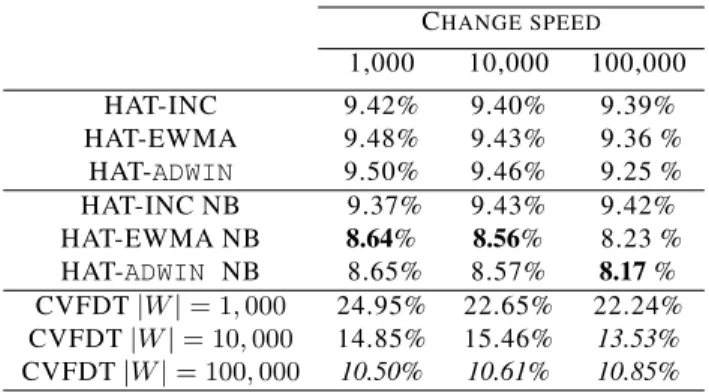
The on-line error rates are shown in Table 3. Observe that, in contrast to previous experiments, HAT-EWMA and HAT-ADWIN do much better than HAT-INC, when using NB at the leaves. We believe this will happen often in the case of gradual changes, because gradual changes will be detected earlier in individual attributes than in the overall error rate.
We test Hoeffding Adaptive Trees on two real datasets in two different ways: with and without concept drift. We tried some of the largest UCI datasets [1], and report results on Adult and Poker-Hand. For the Covertype and Census-Income datasets, the results we obtained with our method were essentially the same as for CVFDT (ours did better by fractions of 1% only) – we do not claim that our method is always better than CVFDT, but this confirms our belief that it is never much worse.
Table 3: On-line errors of Hyperplane Experiments with gradual concept drift
CHANGE SPEED 1,000 10,000 100,000 HAT-INC 9.42% 9.40% 9.39% HAT-EWMA 9.48% 9.43% 9.36 % HAT-ADWIN 9.50% 9.46% 9.25 % HAT-INC NB 9.37% 9.43% 9.42% HAT-EWMA NB 8.64% 8.56% 8.23 % HAT-ADWIN NB 8.65% 8.57% 8.17% CVFDT|W|= 1,000 24.95% 22.65% 22.24% CVFDT|W|= 10,000 14.85% 15.46% 13.53% CVFDT|W|= 100,000 10.50% 10.61% 10.85%
An important problem with most of the real-world benchmark data sets is that there is little concept drift in them [23] or the amount of drift is unknown, so in many research works, concept drift is introduced artificially. We simulate concept drift by ordering the datasets by one of its attributes, theeducationattribute for Adult, and the first (un-named) attribute for Poker-Hand. Note again that while us-ing CVFDT one faces the question of which parameter val-ues to use, our method just needs to be told “go” and will find the right values online.
The Adult dataset aims to predict whether a person makes over 50k a year, and it was created based on census data. Adult consists of 48,842 instances, 14 attributes (6 continuous and 8 nominal) and missing attribute values. The Poker-Hand dataset consists of 1,025,010 instances and 11 attributes. Each record of the Poker-Hand dataset is an example of a hand consisting of five playing cards drawn from a standard deck of 52. Each card is described using two attributes (suit and rank), for a total of 10 predictive attributes. There is one Class attribute that describes the ”Poker Hand”. The order of cards is important, which is why there are 480 possible Royal Flush hands instead of 4.
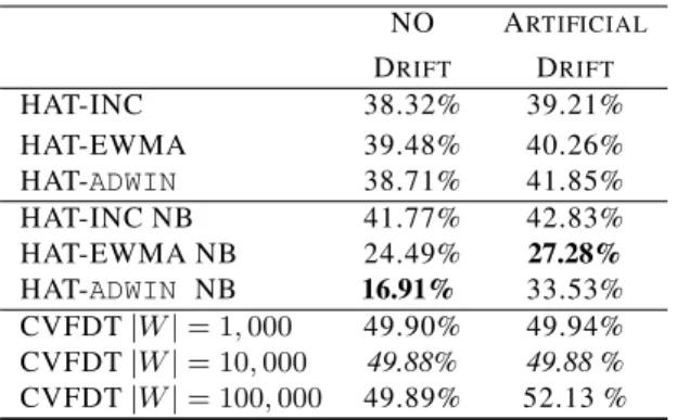
Table 4 shows the results on Poker-Hand dataset. It can be seen that CVFDT remains at 50% error, while the dif-ferent variants of Hoeffding Adaptive Trees are mostly be-low 40% and one reaches 17% error only. In Figure 5 we compare HWT-ADWIN error rate to CVFDT using different window sizes. We observe that CVFDT on-line error de-creases when the example window size inde-creases, and that HWT-ADWIN on-line error is lower for all window sizes. 7 Time and memory
In this section, we discuss briefly the time and memory performance of Hoeffding Adaptive Trees. All programs were implemented in C modifying and expanding the version of CVFDT available from the VFML [14] software web page. We have slightly modified the CVFDT implementation
10% 12% 14% 16% 18% 20% 22% 1.000 5.000 10.000 15.000 20.000 25.000 30.000 O n -l in e E rr o r CVFDT HWT-ADWIN
Figure 5: On-line error on UCI Adult dataset, ordered by the educationattribute. 0 0,5 1 1,5 2 2,5 3 3,5 CVFDT w=1,000 CVFDT w=10,000 CVFDT w=100,000
HAT-INC HAT-EWMA HAT-ADWIN M e m o ry ( M b ) 1000 10000 100000
Figure 6: Memory used on SEA Concepts experiments
Table 4: On-line classification errors for CVFDT and Ho-effding Adaptive Trees on Poker-Hand data set.
NO ARTIFICIAL DRIFT DRIFT HAT-INC 38.32% 39.21% HAT-EWMA 39.48% 40.26% HAT-ADWIN 38.71% 41.85% HAT-INC NB 41.77% 42.83% HAT-EWMA NB 24.49% 27.28% HAT-ADWIN NB 16.91% 33.53% CVFDT|W|= 1,000 49.90% 49.94% CVFDT|W|= 10,000 49.88% 49.88 % CVFDT|W|= 100,000 49.89% 52.13 % 0 50 100 150 200 250 300 CVFDT w=1,000 CVFDT w=10,000 CVFDT w=100,000
HAT-INC HAT-EWMA HAT-ADWIN N u m b e r o f N o d e s 1000 10000 100000
Figure 7: Number of Nodes used on SEA Concepts experi-ments
to follow strictly the CVFDT algorithm explained in the original paper by Hulten, Spencer and Domingos [13]. The experiments were performed on a 2.0 GHz Intel Core Duo PC machine with 2 Gigabyte main memory, running Ubuntu 8.04.
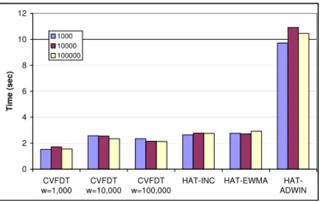
Consider the experiments on SEA Concepts, with differ-ent speed of changes:1,000,10,000and100,000. Figure 6 shows the memory used on these experiments. As expected by memory complexity described in section 5.2, HAT-INC and HAT-EWMA, are the methods that use less memory. The reason for this fact is that they don’t keep examples in mem-ory as CVFDT, and that they don’t storeADWIN data for all attributes, attribute values and classes, as HAT-ADWIN. We have used the default10,000for the amount of window ex-amples kept in memory, so the memory used by CVFDT is essentially the same forW = 10,000 andW = 100,000, and about 10 times larger than the memory used by
HAT-0 2 4 6 8 10 12 CVFDT w=1,000 CVFDT w=10,000 CVFDT w=100,000
HAT-INC HAT-EWMA HAT-ADWIN T im e ( s e c ) 1000 10000 100000
Figure 8: Time on SEA Concepts experiments
INC memory.
Figure 7 shows the number of nodes used in the experi-ments of SEA Concepts. We see that the number of nodes is similar for all methods, confirming that the good results on memory of HAT-INC is not due to smaller size of trees.
Finally, with respect to time we see that CVFDT is still the fastest method, but HAT-INC and HAT-EWMA have a very similar performance to CVFDT, a remarkable fact given that they are monitoring all the change that may occur in any node of the main tree and all the alternate trees. HAT-ADWIN increases time by a factor of 4, so it is still usable if time or data speed is not the main concern.
8 Related Work
It is impossible to review here the whole literature on deal-ing with time evolvdeal-ing data in machine learndeal-ing and data mining. Among those using fixed-size windows, the work of Kifer et al. [17] is probably the closest in spirit toADWIN. They detect change by keeping two windows of fixed size, a “reference” one and “current” one, containing whole exam-ples. The focus of their work is on comparing and imple-menting efficiently different statistical tests to detect change, with provable guarantees of performance.
Among the variable-window approaches, best known are the work of Widmer and Kubat [25] and Klinkenberg and Joachims [18]. These works are essentially heuristics and are not suitable for use in data-stream contexts since they are computationally expensive. In particular, [18] checks all subwindows of the current window, likeADWINdoes, and is specifically tailored to work with SVMs. The work of Last [19] uses info-fuzzy networks or IFN, as an alternative to learning decision trees. The change detection strategy is embedded in the learning algorithm, and used to revise parts
of the model, hence not easily applicable to other learning methods.
Tree induction methods exist for incremental settings: ITI [24], or ID5R [16]. These methods constructs trees using a greedy search, re-structuring the actual tree when new information is added. More recently, Gama, Fernandes and Rocha [8] presented VFDTc as an extension to VFDT in three directions: the ability to deal with continous data, the use of Na¨ıve Bayes techniques at tree leaves and the ability to detect and react to concept drift, by continously monitoring differences between two class-distribution of the examples: the distribution when a node was built and the distribution in a time window of the most recent examples.
Ultra Fast Forest of Trees (UFFT) algorithm is an algo-rithm for supervised classification learning, that generates a forest of binary trees, developed by Gama, Medas and Rocha [10] . UFFT is designed for numerical data. It uses analytical techniques to choose the splitting criteria, and the informa-tion gain to estimate the merit of each possible splitting-test. For multi-class problems, the algorithm builds a binary tree for each possible pair of classes leading to a forest-of-trees.
The UFFT algorithm maintains, at each node of all decision trees, a Na¨ıve Bayes classifier. Those classifiers were constructed using the sufficient statistics needed to evaluate the splitting criteria when that node was a leaf. After the leaf becomes a node, all examples that traverse the node will be classified by the Na¨ıve Bayes. The basic idea of the drift detection method is to control this error rate. If the distribution of the examples is stationary, the error rate of Na¨ıve Bayes decreases or stabilizes. If there is a change on the distribution of the examples the Na¨ıve Bayes error increases.
The system uses DDM, the drift detection method pro-posed by Gama et al. [9] that controls the number of errors produced by the learning model during prediction. It com-pares the statistics of two windows: the first one contains all the data, and the second one contains only the data from the beginning until the number of errors increases. Their method doesn’t store these windows in memory. It keeps only statis-tics and a window of recent examples stored since a warning level triggered. Details on the statistical test used to detect change among these windows can be found in [9].
DDM has a good behaviour detecting abrupt changes and gradual changes when the gradual change is not very slow, but it has difficulties when the change is slowly grad-ual. In that case, the examples will be stored for long time, the drift level can take too much time to trigger and the ex-amples memory can be exceeded.
9 Conclusions and Future Work
We have presented a general adaptive methodology for min-ing data streams with concept drift, and and two decision tree algorithms. We have proposed three variants of
Hoeffd-ing Adaptive Tree algorithm, a decision tree miner for data streams that adapts to concept drift without using a fixed sized window. Contrary to CVFDT, they have theoretical guarantees of performance, relative to those of VFDT.
In our experiments, Hoeffding Adaptive Trees are al-ways as accurate as CVFDT and, in some cases, they have substantially lower error. Their running time is similar in HAT-EWMA and HAT-INC and only slightly higher in HAT-ADWIN, and their memory consumption is remarkably smaller, often by an order of magnitude.
We can conclude that HAT-ADWIN is the most power-ful method, but HAT-EWMA is a faster method that gives approximate results similar to HAT-ADWIN. An obvious fu-ture work is experimenting with the exponential smoothing factorαof EWMA methods used in HAT-EWMA.
We would like to extend our methodology to ensemble methods such as boosting, bagging, and Hoeffding Option Trees. {M}assive{O}nline{A}nalysis [12] is a framework for online learning from data streams. It is closely related to the well-known WEKA project, and it includes a collection of offline and online as well as tools for evaluation. In par-ticular, MOA implements boosting, bagging, and Hoeffding Trees, both with and without Na¨ıve Bayes classifiers at the leaves. Using our methodology, we would like to show the extremely small effort required to obtain an algorithm that handles concept and distribution drift from one that does not. References
[1] D.J. Newman A. Asuncion. UCI machine learning repository, 2007.
[2] Albert Bifet and Ricard Gavald`a. Kalman filters and adaptive windows for learning in data streams. InDiscovery Science, pages 29–40, 2006.
[3] Albert Bifet and Ricard Gavald`a. Learning from time-changing data with adaptive windowing. InSIAM
Interna-tional Conference on Data Mining, 2007.
[4] Albert Bifet and Ricard Gavald`a. Mining adaptively frequent closed unlabeled rooted trees in data streams. In14th ACM SIGKDD International Conference on Knowledge Discovery
and Data Mining, 2008.
[5] L. Breiman, J. Friedman, R. Olshen, and C. Stone.
Classifica-tion and Regression Trees. Wadsworth and Brooks, Monterey,
CA, 1994.
[6] M. Datar, A. Gionis, P. Indyk, and R. Motwani. Maintaining stream statistics over sliding windows. SIAM Journal on
Computing, 14(1):27–45, 2002.
[7] Pedro Domingos and Geoff Hulten. Mining high-speed data streams. InKnowledge Discovery and Data Mining, pages 71–80, 2000.
[8] J. Gama, R. Fernandes, and R. Rocha. Decision trees for mining data streams.Intell. Data Anal., 10(1):23–45, 2006. [9] J. Gama, P. Medas, G. Castillo, and P. Rodrigues. Learning
with drift detection. InSBIA Brazilian Symposium on
Artifi-cial Intelligence, pages 286–295, 2004.
[10] J. Gama, P. Medas, and R. Rocha. Forest trees for on-line data. InSAC ’04: Proceedings of the 2004 ACM symposium
on Applied computing, pages 632–636, New York, NY, USA,
2004. ACM Press.
[11] Geoffrey Holmes, Richard Kirkby, and Bernhard Pfahringer. Stress-testing hoeffding trees. In PKDD, pages 495–502, 2005.
[12] Geoffrey Holmes, Richard Kirkby, and Bern-hard Pfahringer. MOA: Massive Online
Analy-sis. http://sourceforge.net/projects/
moa-datastream. 2007.
[13] G. Hulten, L. Spencer, and P. Domingos. Mining time-changing data streams. In7th ACM SIGKDD Intl. Conf. on
Knowledge Discovery and Data Mining, pages 97–106, San
Francisco, CA, 2001. ACM Press.
[14] Geoff Hulten and Pedro Domingos. VFML – a toolkit for mining high-speed time-changing data streams.
http://www.cs.washington.edu/dm/vfml/.
2003.
[15] K. Jacobsson, N. M¨oller, K.-H. Johansson, and H. Hjalmars-son. Some modeling and estimation issues in control of het-erogeneous networks. In16th Intl. Symposium on
Mathemat-ical Theory of Networks and Systems (MTNS2004), 2004.
[16] Dimitrios Kalles and Tim Morris. Efficient incremental induction of decision trees. Machine Learning, 24(3):231– 242, 1996.
[17] D. Kifer, S. Ben-David, and J. Gehrke. Detecting change in data streams. InProc. 30th VLDB Conf., Toronto, Canada, 2004.
[18] R. Klinkenberg and T. Joachims. Detecting concept drift with support vector machines. InProc. 17th Intl. Conf. on Machine
Learning, pages 487 – 494, 2000.
[19] M. Last. Online classification of nonstationary data streams.
Intelligent Data Analysis, 6(2):129–147, 2002.
[20] Ross J. Quinlan. C4.5: Programs for Machine Learning
(Morgan Kaufmann Series in Machine Learning). Morgan
Kaufmann, January 1993.
[21] T. Sch¨on, A. Eidehall, and F. Gustafsson. Lane departure detection for improved road geometry estimation. Technical Report LiTH-ISY-R-2714, Dept. of Electrical Engineering, Link¨oping University, SE-581 83 Link¨oping, Sweden, Dec 2005.
[22] W. Nick Street and YongSeog Kim. A streaming ensemble algorithm (sea) for large-scale classification. In KDD ’01: Proceedings of the seventh ACM SIGKDD international
con-ference on Knowledge discovery and data mining, pages 377–
382, New York, NY, USA, 2001. ACM Press.
[23] Alexey Tsymbal. The problem of concept drift: Definitions and related work. Technical Report TCD-CS-2004-15, De-partment of Computer Science, University of Dublin, Trinity College, 2004.
[24] Paul E. Utgoff, Neil C. Berkman, and Jeffery A. Clouse. Decision tree induction based on efficient tree restructuring.
Machine Learning, 29(1):5–44, 1997.
[25] G. Widmer and M. Kubat. Learning in the presence of con-cept drift and hidden contexts. Machine Learning, 23(1):69– 101, 1996.