c
APPLICATION OF GENERATIVE MODELS IN SPEECH PROCESSING TASKS
BY
YANG ZHANG
DISSERTATION
Submitted in partial fulfillment of the requirements
for the degree of Doctor of Philosophy in Electrical and Computer Engineering in the Graduate College of the
University of Illinois at Urbana-Champaign, 2017
Urbana, Illinois
Doctoral Committee:
Professor Mark A. Hasegawa-Johnson, Chair Professor Thomas S. Huang
Professor Steven E. Levinson
ABSTRACT
Generative probabilistic and neural models of the speech signal are shown to be effective in speech synthesis and speech enhancement, where generating natural and clean speech is the goal. This thesis develops two probabilis-tic signal processing algorithms based on the source-filter model of speech production, and two based on neural generative models of the speech signal. They are a model-based speech enhancement algorithm with ad-hoc micro-phone array, called GRAB; a probabilistic generative model of speech called PAT; a neural generative F0 model called TEReTA; and a Bayesian enhance-ment network, call BaWN, that incorporates a neural generative model of speech, called WaveNet. PAT and TEReTA aim to develop better gener-ative models for speech synthesis. BaWN and GRAB aim to improve the naturalness and noise robustness of speech enhancement algorithms.
Probabilistic Acoustic Tube (PAT) is a probabilistic generative model for speech, whose basis is the source-filter model. The highlights of the model are threefold. First, it is among the very first works to build a complete probabilistic model for speech. Second, it has a well-designed model for the phase spectrum of speech, which has been hard to model and often neglected. Third, it models the AM-FM effects in speech, which are perceptually sig-nificant but often ignored in frame-based speech processing algorithms. Ex-periments show that the proposed model has good potential for a number of speech processing tasks.
TEReTA generates pitch contours by incorporating a theoretical model of pitch planning, the piece-wise linear target approximation (TA) model, as the output layer of a deep recurrent neural network. It aims to model semantic variations in the F0 contour, which is challenging for existing network. By combining the TA model, TEReTA is able to memorize semantic context and capture the semantic variations. Experiments on contrastive focus verify TEReTA’s ability in semantics modeling.
BaWN is a neural network based algorithm for single-channel ment. The biggest challenges of the neural network based speech enhance-ment algorithm are the poor generalizability to unseen noises and unnatu-ralness of the output speech. By incorporating a neural generative model, WaveNet, in the Bayesian framework, where WaveNet predicts the prior for speech, and where a separate enhancement network incorporates the likeli-hood function, BaWN is able to achieve satisfactory generalizability and a good intelligibility score of its output, even when the noisy training set is small.
GRAB is a beamforming algorithm for ad-hoc microphone arrays. The task of enhancing speech with ad-hoc microphone array is challenging be-cause of the inaccuracy in position and interference calibration. Inspired by the source-filter model, GRAB does not rely on any position or interference calibration. Instead, it incorporates a source-filter speech model and min-imizes the energy that cannot be accounted for by the model. Objective and subjective evaluations on both simulated and real-world data show that GRAB is able to suppress noise effectively while keeping the speech natural and dry.
Final chapters discuss the implications of this work for future research in speech processing.
ACKNOWLEDGMENTS
I would like to acknowledge my graduate advisor, Professor Mark Hasegawa-Johnson, who has given me lots of research opportunities, guidance and in-sights. His broad knowledge and research attitude deeply cultivated me to become an independent, innovative and upright researcher.
I would also like to acknowledge my undergraduate advisor, Professor Zhi-jian Ou, and my internship mentors, Dr. Nasser Nasrabadi, Dr. Gautham Mysore, and Dr. Dinei Florˆencio, who have deeply inspired me through-out the continuing collaborations and contributed significantly to my thesis research.
Finally I would like to acknowledge my research collaborators, Mr. Shiyu Chang, Mr. Kaizhi Qian, Mr. Xuesong Yang, Mr. Tom Paine, and Ms. Xiayu Chen, for their strong academic support and encouragement.
TABLE OF CONTENTS
CHAPTER 1 MOTIVATION . . . 1
1.1 The Challenges . . . 2
1.2 Generative Models of Speech . . . 3
CHAPTER 2 BACKGROUND . . . 5
2.1 Introduction . . . 5
2.2 The Source-Filter Model and Speech Production . . . 6
2.3 Models for Source . . . 13
2.4 Models for Filter . . . 16
CHAPTER 3 PROBABILISTIC GENERATIVE MODEL OF SPEECH . . . 21
3.1 Introduction . . . 21
3.2 Related Work . . . 24
3.3 Probabilistic Acoustic Tube . . . 25
3.4 Monte-Carlo Inference . . . 33
3.5 Experiments and Analyses . . . 43
3.6 Discussions . . . 50
CHAPTER 4 TEXT-TO-SEMANTICS F0 MODELING . . . 52
4.1 Introduction . . . 52
4.2 Target Approximation F0 Model . . . 57
4.3 Text-Embedded Recurrent Target Approximation . . . 61
4.4 The Contrastive Focus Corpus . . . 65
4.5 Experiments and Analysis . . . 67
4.6 Conclusions and Future Directions . . . 74
CHAPTER 5 BAYESIAN WAVENET FOR SPEECH ENHANCE-MENT . . . 75
5.1 Introduction . . . 75
5.2 The Model Architecture . . . 77
5.3 Training the Model . . . 81
5.4 Experiments . . . 83
CHAPTER 6 MODEL-BASED SPEECH ENHANCEMENT WITH
AD-HOC MICROPHONE ARRAY . . . 89
6.1 Introduction . . . 89
6.2 Related Works . . . 91
6.3 Glottal Residual Assisted Beamforming . . . 91
6.4 Estimating Clean Speech LPC Residual . . . 94
6.5 Experiments . . . 99
6.6 Conclusion and Future Directions . . . 105
CHAPTER 7 DISCUSSION . . . 106
7.1 Contributions to Natural Speech . . . 106
7.2 Combination with Pattern Recognition Techniques . . . 109
CHAPTER 8 CONCLUSION . . . 112
CHAPTER 1
MOTIVATION
Speech is one of the most distinctive characteristics of human beings, and one of the most convenient means of communication. Therefore, a common goal of today’s speech processing technology is to enable people to interact with computer conveniently using speech. To accomplish this, two common problems have to be tackled: (1) How to make computers understand hu-man speech better, and (2) How to make computers generate speech that is perceived as natural to human users. The scope of this thesis falls into the second challenge.
Specifically, there are two tasks that involve generating natural speech, speech synthesis and speech enhancement. Speech synthesis refers to the task of generating natural-sounding speech from text and/or other linguistic annotations. In speech synthesis, the concept of naturalness can be divided into two levels. The first level is the acoustic level. Speech that sounds acoustically natural should have a human-like timbre, and be free of discon-tinuities or artifacts. The second level is the prosodic level, which refers to the intonation and rhythm of speech. Speech that sounds natural in prosody should have a human-like intonation, proper emphasis and variations. Mod-ern speech synthesizers typically consist of an acoustic model and a prosody model, and thus the task of making speech natural in both levels can be decomposed into improving the quality of the two respective models.
The second task that requires natural sounding output is speech enhance-ment. Speech enhancement is a broad class of speech processing tasks that involve improving the quality of the corrupted input speech. Speech denois-ing, in particular, refers to the task that removes any unwanted noise present in speech. Speech dereverberation refers to the task that removes reverber-ation present in speech. There are two types of speech enhancement tasks: single-channel, where the noisy speech is picked by one sensor only, and multi-channel, where the noisy speech are recorded by microphone arrays of
ad-hoc sensor networks. The output of the speech enhancement algorithms can have two purposes: one is for noise-robust speech recognition, and the other is for human consumption, such as in noise-free teleconferencing. The former one does not require the speech to be natural, but in the latter pur-pose, naturalness plays a big role. It is shown that people prefer noisy but natural speech than clean but unnatural ones [1].
1.1
The Challenges
However, despite the importance of naturalness in these speech processing tasks, generating natural speech is a challenging problem for computers. This is because, unlike the problem of recognizing speech, where the performance can usually be quantified as accuracy, the concept of “naturalness” is sub-jective and can hardly be turned into a quantifiable measure. Without this quality it is difficult to convert the task into a pattern recognition problem digestible to computers.
There have been many efforts of quantifying speech naturalness. A class of metrics are proposed based on human subjective evaluation. The mean opin-ion score (MOS) [2] is a 1-5 score reflecting the quality of the media assigned by human participants. Crowd MOS [3] is a variant of MOS that is applica-ble to crowd-sourcing scenarios. Another modified version of MOS has been proposed specifically for speech synthesis systems [4]. Multiple stimuli with hidden reference and anchor (MUSHRA) is a testing protocol that properly controls participant heterogeneity by introducing anchors. However, these subjective measures are only useful in evaluating speech processing systems, not in training them. Other research efforts have been made to develop prox-ies for the objective measures, including peceptual speech quality Measure (PSQM) [5], perceptual evaluation of speech quality (PESQ) [6], bark spec-tral distortion (BSD) [7,8], and short-time objective intelligibility (STOI) [9]. A number of works aim to predict subjective scores using a set of objective measures [10–12]. Yet, they are still designed primarily for evaluation pur-poses. It is still difficult to apply these objective proxies directly to training speech processing systems.
Therefore, here comes our question: Now that training speech processing systems with speech quality measures is difficult, how can we design
algo-rithms that produce natural sounding outputs?
1.2
Generative Models of Speech
One possible solution to generate natural sounding speech output is through the application of generative models of speech. The term generative model has different interpretations in different fields. In this thesis, generative mod-els refer to modmod-els that define the sample space for speech, which includes both acoustic models and prosody models. Many speech generative models are well motivated by the actual production process of speech. For example, the source-filter model [13] is a generative model for acoustic speech signal that emulates glottal vibration (as source) and articulator positioning in the vocal tract (as filter). The target approximation model [14] is a prosody model for F0 contour that incorporates the constraint of articulatory mo-tors. With the rapid development of deep learning, the deep learning based generative models of speech have also gained wide attention. WaveNet [15] is an acoustic model of speech that applies dilated convolution neural net-work. SEGAN [16] introduces a generative model of acoustic speech using generative adversarial network (GAN) [17]. It has been shown that these gen-erative models of speech are capable of generating natural sounding speech. Therefore, by incorporating generative models of speech into various speech processing systems, we expect to improve naturalness of the output speech.
There are, however, two questions to answer before applying generative models. The first question is: How can generative contribute to the natu-ralness of output speech? As mentioned, the speech processing tasks we are interested in are speech synthesis and speech enhancement. Although the common goal is to produce natural sounding output, each task has its own settings. How can generative models help improving speech naturalness in the different settings, and are they effective?
The second question to answer is more at a methodology level: How do we combine the generative models with different machine learning techniques? Machine learning techniques are essential in speech processing systems. For example, in speech synthesis systems, machine learning is applied to estimate synthesis parameters; in speech enhancement systems, machine learning is applied to infer the clean speech. In the meantime, machine learning includes
a wide variety of methods, including but not limited to simple least-square approaches, Bayesian approaches and deep neural networks. Can generative models find their way to these different approaches?
In this thesis, we are going to investigate in these two dimensions. First, we explore the role of generative models in different speech processing tasks, including speech synthesis and speech enhancement. Specifically, for the acoustic modeling in speech synthesis, chapter 3 introduces a probabilistic source-filter model that improves over the existing acoustic models by intro-ducing a better model for phase and anti-causal component. For the prosodic modeling in speech synthesis, chapter 4 introduces an F0 model that com-bines the target approximation model and deep learning techniques, which is among the first F0 models capable of capturing contrastive focus directly from text. For single-channel speech enhancement, chapter 5 introduces a deep learning algorithm that incorporates WaveNet as the speech prior, guid-ing the algorithms to produce speech like output. For multi-channel speech enhancement, chapter 6 introduce a beamforming algorithm, which is guided by the source-filter model, and which is able to generate surprisingly natural-sounding enhancement output. Although the tasks vary, the algorithms all incorporates a generative model – the source-filter model for chapters 3 and 6, the WaveNet model for chapter 5, and the target approximation model for 4. The purpose of introducing these generative models are all to improve the quality of output speech waveform or prosody. More details will be discussed in the respective chapters.
In the meantime, different ways to combine machine learning techniques with these generative models are explored. Specifically, to perform parameter estimation for speech synthesis tasks, Monte-Carlo approaches are used in chapter 3, and simple gradient descent are applied for chapter 4. To perform inference for speech enhancement tasks, a neural network in the Bayesian framework is applied in chapter 5, and an iterative least-square approach is applied in chapter 6. Further discussions on the pros and cons of different techniques combined with generative models are given in chapter 7.
The remainder of the thesis is organized as follows. Chapter 2 introduces background on the source-filter model. Chapters 3-6 introduce the works that involve generative models in speech synthesis and enhancement tasks. Chapter 7 discusses the roles of the generative models, as well as the machine learning techniques combined with these models.
CHAPTER 2
BACKGROUND
This chapter provides an overview of the source-filter model as the most tra-ditional yet popular generative model of speech, which forms the theoretical basis for chapters 3 and 6. It is organized as follows. Sections 2.1 briefly introduces the source-filter model and its significance in various speech pro-cessing tasks. Section 2.2 provides an overview of the source-filter model. Sections 2.3 and 2.4 discuss different models for the source and the filter respectively.
2.1
Introduction
Generative models [18] refer to a broad class of models that attempt to char-acterize the distribution of variables of interest. Generative model are often compared with discriminative models as another popular category, which, in classification tasks, determines the boundary of features belonging to dif-ferent classes, instead of modeling the potentially complicated distribution within each class. Both classes of models have their own merits. Discrimina-tive models are more cost-effecDiscrimina-tive and provide better performance in classi-fication tasks, partly because the complexity of modeling the class boundary is much lower than that of modeling the entire distribution, and the class boundary is all we need to know for classification.
On the other hand, generative models are indispensable when generating the data itself is part of the task. In speech processing, in particular, such tasks include speech synthesis, speech manipulation, speech enhancement, source separation, etc. A strong generative model incorporated could help the algorithm to produce natural sounding speech.
There are a variety of generative models for speech. Linear coding based models are widely used for speech enhancement and source separation,
in-cluding principal component analysis (PCA) [19–21], non-negative matrix factorization (NMF) [22, 23], independent component analysis (ICA) [24, 25] and sparse coding and dictionary learning [26–28]. Another commonly used strategy uses probabilistic models on time-frequency representation of speech frames [29]. Other unsupervised models include vector quantization [30] and clustering [31]. These models are more to the data-driven end, with little domain knowledge of speech applied.
The source-filter model, on the other hand, is one of the most popular signal processing generative models of speech that heavily utilize domain knowledge of speech. Although it has long been proposed [32], it still lends valuable insights and theoretical foundations to many more sophisticated speech models today. Also, it provides handy and effective solutions to many challenging speech-processing problems, such as multi-channel enhancement, with performance matching or even exceeding that of many modern tech-niques. Readers will better appreciate the power of source-filter model in chapters 3 and 6, which discuss two works that are both based on the source-filter model.
2.2
The Source-Filter Model and Speech Production
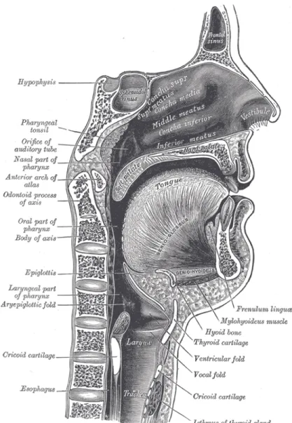
The source-filter model emulates the actual human speech production pro-cess, so it is useful to have an overview on how speech is produced. Roughly speaking, the human speech system consists of three parts: lungs, larynx and vocal tract. The lungs provide power supplies by pushing the air up-ward through the trachea. The larynx serves as a modulator that modulates the airflow, providing either a periodic (for the voiced state) or a noisy airflow (for the unvoiced state) sound source. The vocal tract acts like a resonator that “colors” the sound by shaping the spectrum of the sound source. In some occasions, the vocal tract can also serve as a sound source by forming constriction or boundaries within and forcing the airflow to form high speed turbulence. Finally, the air wave radiates out from the lips and becomes the speech signal.Figure 2.1 shows an anatomical view of the larynx and the vocal tract. The following subsections introduce these two parts in greater detail.
Figure 2.1: Human speech production.a
a“Sagittalmouth”. Licensed under Public Domain via Wikimedia Commons
2.2.1
Larynx
The main function of the larynx is to control the vocal folds, or vocal chords. The vocal folds are a pair of aligned flesh masses, between which the airflow passes. The tension of the vocal folds is controlled by the larynx, which can form three different states: breathing, unvoiced and voiced states.
In the breathing state, the vocal folds are completely relaxed, and the airflow can pass through freely. The breathing state corresponds to no speech activity. In the unvoiced state, the vocal folds are tensor and closer together, creating resistance for the airflow that passes through, which forms high speed turbulence called “aspiration”. Unvoiced speech refers to the speech driven by such aspiration, and is present in some consonants and “whispered” speech.
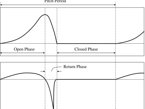
The voiced state is the dominant speech state in terms of duration and energy. In the voiced state, the vocal folds are even tenser and closer together, such that the airflow passing through can drive a sustainable oscillation. The oscillation can be divided into three phases: open phase, return phase and closed phase. Figure 2.2 upper panel shows a typical airflow velocity in each of these three phases. In the open phase, the vocal folds are pushed wider due to the accumulated air pressure at one end, and thus there is an increase in airflow velocity. In the glottal return phase, the airflow velocity becomes so large that the air pressure starts to decrease (Bernoulli principle). The air pressure outside the vocal folds exceeds that of the inside, pushing the vocal folds toward each other, and slowing down the airflow. Finally, in the closed phase, the vocal folds are so close to each other that they shut the pass-way in between. The airflow is completely stopped and starts to accumulate at one end of the vocal folds until the pressure is large enough to push the vocal folds open again, which then starts the next open phase. The two-mass model [33], as well as other more sophisticated physical models, has been proposed to study this process analytically.
Each consecutive open phase, return phase and closed phase forms a glot-tal cycle, the duration of which is called the fundamental period, and the frequency of which is called the fundamental frequency, or F0. F0 is gen-erally perceived as pitch frequency, although the two terms cannot be used interchangeably.
Open Phase Closed Phase
Return Phase Pitch Period
Figure 2.2: Typical shape of the glottal wave. Upper panel: airflow velocity at the glottis. Lower panel: first-order derivative of the airflow velocity at the glottis.
unvoiced and voiced states. Breathy speech, for example, refers to a glottal state where the distance of the vocal folds falls between the unvoiced and voiced state – they are farther apart than in the regular voiced state, but close enough to form an oscillation. Such voiced state is characterized by long open phase, short closed phase and strong aspiration energy. Creaky voice is another voicing state where the vocal folds are so tense that only a portion of them vibrates, resulting in what is perceived as harsh-sounding voice with high and irregular pitch. Vocal fry [34, 35] refers to the other extreme case where the vocal folds are so relaxed that there is a secondary pulse before the main pulse in the open phase, resulting in an abnormally low and irregular pitch. Diplophonic voice [36] is also characterized by a secondary pulse in a low-pitched speaker, but it is separated from the primary pulse. Yet these voice states are not as common as the unvoiced and voiced states, so in the remainder of the chapter the primary focus is on the latter two states.
2.2.2
Vocal Tract
The vocal tract consists of an oral tract and a nasal tract. The oral tract plays the dominating role in shaping the spectrum of speech, and therefore we will first introduce models for the oral tract, and then consider the effect of incorporating the nasal tract.
Rabiner and Schafer [37] proposed an acoustic tube model for the air wave propagation inside the oral tract. The acoustic tube model makes the fol-lowing simplifying assumptions.
• The oral tract can be approximated by a concatenation of N uniform tubes, whose cross-sectional areas are {Ak};
• The sound wave travels as planar sound waves and propagates longitu-dinally;
• The walls of the tubes are lossless – there is no energy dissipation of any form, including friction, wall vibration and heat radiation.
Define the normal direction to the cross sections of the tubes as the x direc-tion. x = 0 corresponds to the glottis position, and x = L corresponds to the lips position. Assume each of the uniform tube is of length ∆L. Denote
p(x, t) and v(x, t) as the air pressure and velocity at location x and time t
respectively.1
Now we also need to introduce the boundary condition. Define the impedance at the glottis and at the lips as
Zr(Ω) = P(L,Ω) V(L,Ω) Zg(Ω) = P(0,Ω) V(L,Ω) (2.1)
where P(x,Ω) and V(x,Ω) are the Fourier transforms of p(x, t) and v(x, t) respectively.
It can be shown [38,39] that the impedance at the lips, a.k.a. the radiation impedance, can be modeled as a parallel circuit
Zr(Ω) = jΩLrRr
Rr+jΩLr
(2.2) and the impedance at the glottis can be modeled as a serial circuit
Zg(Ω) =Rg +jΩLg (2.3)
Then, by solving the wave equation [40] − ∂p ∂x =ρ ∂v ∂t − ∂p ∂t =ρc 2∂v ∂x. (2.4)
subject to the boundary conditions in equations (2.2) and (2.3), and by proper discretization, the following conclusion can be obtained
H(z) = VL(z) Vg(z) = Az −N/2 1−PN k=1akz−k (2.5) where VL(z) is the Z-transform of discretized v(L, t), and Vg(z) is the Z-transform of discretized vg(t). If Zg(Ω) = +∞, {ak} can be determined by the Levinson’s recursion [37]. The Levinson’s recursion can prove that as 1The wave is assumed to be a planar wave so a single coordinate xsuffices to charac-terize the wave.
long as the reflection coefficients
rk =
Ak+1−Ak
Ak+1+Ak
<1 (2.6)
which is always the case, the poles of H(z) are all within the unit circle. Equation (2.5) implies that the oral tract can be approximated as an all-pole system with the transfer function H(z). However, if the nasal tract is taken into account, which can also be approximated as an all-pole system, the entire vocal tract is not necessarily all-pole, but a general system with poles and zeros. Nevertheless, the all-pole approximation is still a popular assumption on the vocal tract system.
2.2.3
The Source-Filter Model Framework
Now we are ready to develop the framework of the source-filter model. In practice, speech is measured as the pressure wave at the output, p(L, t), whose Z-transform is denoted as PL(z), or more intuitively as S(z) to echo the word “speech”. Therefore, the speech signal can be represented as
S(z) =PL(z) =Vg(z)VL(z) Vg(z) PL(z) VL(z) =Vg(z)H(z)Zr(z) (2.7)
where H(z) is given in equation (2.5). Zr(z) is the impedance at the lips, or the radiation impedance, which is the Z-transform analogue of Zr(Ω) as in equations (2.1) and (2.2) through bilinear transform. It can be shown that, under the empirical values Rr = 128/9π2 and Lr = 31.5×10⁻⁶,
Zr(z)≈1−z−1 (2.8)
which is a first-order differentiator.
The source-filter model merges the radiation impedance Zr(z) into the airflow velocity at the glottis Vg(z). Formally, define
E(z) =Vg(z)Zr(z) (2.9) as the excitation signal, which is essentially the differentiated airflow velocity
at the glottis, which we will call theglottal wave in the remainder of the thesis. Combining equations (2.7) and (2.9), we have
S(z) =E(z)H(z) (2.10) Equation (2.10) is the basic framework of the source-filter model, which as-sumes speech is generated by passing the excitation signal, E(z), through the vocal tract system H(z).
It is also worth mentioning that the actual glottal source and vocal tract have nonlinear interactions, which lead to approximation errors of the source-filter model [41]. Nevertheless these effects are secondary and safe to ignore in most speech processing tasks of interest.
Therefore, further theories of the source-filter model boil down to those for the source and the filter respectively, as will be discussed in the following two sections.
2.3
Models for Source
For unvoiced speech, the source, i.e. turbulence, is stationary noise with an almost flat spectrum, and therefore is approximated by white noise [13].
The major focus is the voiced case. From equation (2.9), the glottal wave is essentially the first-order differentiation of the actual air velocity. Figure 2.2 lower panel shows a typical glottal waveform. We assume for now that the glottal wave is completely periodic. Then
E(z) =P(z)G(z) (2.11) where P(z) is the Z-transform of a periodic pulse train, p[t], whose period is the fundamental period of the glottal excitation, denoted as T0. G(z) is the
Z-transform of the glottal wave within one period, denoted as g[t].
Like the original glottal air velocity,g(t) can be divided into three phases: open phase, return phase and closed phase. The negative peak at the glottal derivative is called glottal closure instant (GCI).
There are many models for this canonical glottal wave. In the following subsections, we will review some of the most influential models.
2.3.1
Rosenberg’s Model
Rosenberg [42] proposed and compared six different models in terms of per-ceptual similarity. The best model can be represented as follows
g[t] = ( t2(t e−t) if 0< t < te =tc 0 if te< t < T0 (2.12) where te is the glottal closure instant. There is one parameter in this model, i.e. te.
2.3.2
KLGLOTT88
Klatt and Klatt [36] proposed an improved version over the Rosenberg’s model, named KLGLOTT88, which can be formulated as
g[t] =b[t]∗f[t] +b[t] (2.13) where b[t] is the base waveform, represented as
b[t] = ( t2(QT 0−t) if 0< t < OT0 0 if OQT0 < t < T0 (2.14)
O is the open quotient of a glottal cycle. f[t] is a low-pass resonator which controls the spectral tilt TL. b[t] is the additive breathiness voice, whose energy is dependent upon O. The model thus has two parameters, O and
TL. A closed-form representation of its spectral shape can be found in [43].
2.3.3
Fujisaki’s Model
Fujisaki and Ljungqvist [44] proposed the following piecewise polynomial models: g[t] = A− 2A+tpα tp + A+tpα tp t 2 if 0< t≤t p α(t−tp) + 3B−2(te−tp)α te−tp − 2B−(te−tp)α (te−tp)3 (t−te+tp) 3 if t p < t≤te C− 2(Ct−B) c (t−te) + C−B (tc−te)2(t−te) 2 if t e< t≤tc β if tc< t≤T0 (2.15)
where
α= 4Atp−6(te−tp)B (te−tp)2−2t2p
, β = Ctc
tc−3(T0−te)
There are six parameters of the model: tp is the time when glottal opening is widest; te is the glottal closure instant; tc is thetime when closed phase starts; A, B and C are shape parameters.
2.3.4
The LF Model
Fant et al. [45] proposed the most popular LF-model, which is a combination of the L-model and F-model [46]. It is described as follows:
g[t] = ( E0eαtsinωgt if 0< t≤te −E0 εtα e−ε(t−te)−e−ε(tc−te) t e < t≤tc (2.16) There are six nominal parameters tp, te, ta, E0, ε and ωg, but with two constraints: one is that g[t] should be continuous at te; the other is that the glottal flow derivative integrates to 0 over a glottal cycle:
Z T0
0
g[t] = 0 Therefore, the number of free parameters is four.
Some spectral properties of the LF-model are discussed in [43, 47].
Fant [48] simplifies the LF-model to have one parameter by introducing some empirical relationship among the original four parameters, which are reorganized as R0 = te T0 , Rg = T0 2tp , Rk= te−tp tp , Rα = tα T0
The merged parameter, denoted as Rd, is defined as
Rd= 1 0.11(0.5 + 1.2Rk) Rk 4Rg +Rα (2.17) The rest of the parameters can be empirically determined as:
Rα = −1 + 4.8Rd 100 , Rk = 22.4 + 11.8Rd 100 , Rg = 0.25Rk 0.11Rd 0.5+1.2R −Rα (2.18)
2.3.5
The All-Pole Models and Causality
There is another important class of models that utilize causality. Throughout a pitch cycle, the GCI location is usually assumed to be where the impulse of P(z) (equation (2.11)) lies, because it is where the glottal wave energy is largest, and where the energy tapers off along both directions, as shown in figure 2.2. Therefore, the glottal open phase and a part of the glottal return phase are responses before the impulse, and thereby correspond to the anti-causal component; the remainder of the glottal return phase is the response after the impulse, and therefore corresponds to the causal component. In the Z plane, anti-causal components correspond to the maximum-phase compo-nents, i.e. poles and zeros outside the unit circle; and causal components correspond to the minimum-phase components, i.e. poles and zeros inside the unit circle. In the cepstral domain, the anti-causal components are left-sided in the quefrency domain, and causal components are right-left-sided. More detailed discussion can be found in section 2.4.
Gardner and Rao [49] observed that the glottal wave can be modeled by the impulse response of a non-causal all-pole filter with the impulse at GCI. It was demonstrated that eight poles are sufficient to approximate the glottal flow. The work in [50, 51] proposes a three-pole model with two anti-causal poles and one causal pole. Drugman et al. [52] released the all-pole constraint and modeled the anti-causal component of the glottal wave with cepstrum, which leads to an effective glottal wave estimation algorithm.
It is worth mentioning that many glottal models suffer from approximation errors. On one hand, there are many special glottal events which are not con-sidered. For instance, vocal fry [35] and diplophonic voice [36], as discussed in section 2.2.1. On the other hand, even for the typical glottal wave, it is shown that [53] there are ripples in the open phase that are not modeled by the canonical shape of the glottal wave. Nevertheless, these glottal models are good enough for many purposes.
2.4
Models for Filter
Two classical models for vocal tract filter are discussed. One is LPC and the other is cepstral coefficients. The rest of this subsection will focus on voiced case.
As discussed in section 2.3, the glottal excitation of voiced-speech is a quasi-periodic signal. Combining equations (2.10) and (2.11) we have
PL(z) =P(z)G(z)H(z) (2.19) LPC and cepstral analysis utilize different characteristics of H(z).
2.4.1
LPC Analysis
LPC (Linear Predicative Coding) analysis rests on the all-pole assumption of speech. It is already discussed in section 2.3.5 thatG(z) can be approximated by an all-pole system with a pair of anti-causal poles and one causal pole. Also, as already shown in section 2.2.2 that H(z) can be well modeled by a causal all-pole system.
The all-pole assumption asserts that speech can be linearly predicted by its previous samples
s[t] = q
X
k=1
aks[t−k] +r[t] (2.20) where r(t) is the prediction residual, which is mathematically analogous to excitation of the all-pole system. {ak}are LPC coefficients, which are math-ematically analogous to denominator polynomial coefficients of the system. q
is the order of autoregression. Formally, taking the Z-transform of equation (2.20) S(z) =L(z)R(z) (2.21) where L(z) = 1 1−a1z−1− · · · −aqz−q (2.22)
S(z) and R(z) are Z-transforms of s[t] andr[t] respectively.
LPC analysis [54] estimates the filter coefficients {ak} by minimizing the expected energy of the residual, i.e.
min
{ak}
=Er[t]2 (2.23)
The expectation operator is a convenient expression under the assumption of ergodicity.
The solution is given by a= Φ−1b (2.24) where a= [a1,· · · , aq]T Φij =E[s[t−i]s[t−j]] b= [E[s[t−1]s[t]],· · · ,E[s[t−q]s[t]]]T
Depending on how the samples outside the analysis window are treated, there are two ways of computing Φ, named the autocorrelation method and the autocovariance method [55]. There is a more efficient algorithm, the Levinson’s recursion [56], whose computation complexity is O(q) instead of
O(q3).
An important question that has yet to be answered is how do L(z) and
R(z) in equation (2.22) correspond to the speech componentsP(z),G(z) and
H(z) in equation (2.21). If there is no meaningful correspondence, then LPC analysis would shed no light on the source or filter information of speech. For-tunately, we have the following conclusion. If the following two assumptions hold:
• the autocorrelation function of Re(τ) = E[e[t]e[t−τ]] = 0, ∀τ ≤q; • G(z)H(z) is an all-pole system or order q;
then the poles of L(z) are all the minimum-phase poles of G(z)H(z), and the conjugate of all the maximum-phase poles of G(z)H(z) (the conjugate of a pole atz isz−1). Accordingly, R(z) is equal to P(z) passing through an
all-pass filter, which consists of all the maximum-phase poles of G(z)H(z), and the corresponding conjugate zeros. The first assumption holds as long as the fundamental period (in # sample points) T0 > q. For 16 kHz speech.
A typical value for q is 13, and T0 usually fall within 2 ms - 10 ms, which
is 32-160 number of sample points. Therefore T0 > q is satisfied. The
second assumption approximately holds by the all-pole models of G(z) and
H(z). Therefore, the correspondence is well justified. Chapter 6 gives a more detailed explanation on this.
2.4.2
Cepstral Analysis
One major disadvantage about LPC analysis is that the all-pole assumption is too strong. Zeros will be introduced, for example, for nasals and nasal-ized vowels [57, 58]. Cepstral analysis is a model that releases the all-pole assumption, but maintains the causality assumption.
Cepstrum is defined as the inverse Z-transform of the logarithm Z-transform. Specifically, take the logarithm of equation (2.19), we have
logS(z) = logP(z) + logG(z) + logH(z) (2.25) Taking the inverse Z-transform of (2.25), we finally have
ˇ
s[ˇn] = ˇp[ˇn] + ˇg[ˇn] + ˇh[ˇn] (2.26) where ˇs[ˇn], ˇp[ˇn], ˇg[ˇn] and ˇh[ˇn] are cepstrums of speech, periodic pulse train, glottal wave within one cycle and vocal tract respectively; ˇn is the index in the quefrency domain.
The ˇp[ˇn], ˇg[ˇn] and ˇh[ˇn] exhibit different characteristics; ˇg[ˇn] and ˇh[ˇn] are represented by poles and zeros. Consider more generally a rational Z-transform of the form
X(z) =Az−r QMi k=1(1−akz−1) QMo k=1(1−bkz) QNi k=1(1−ckz−1) QNo k=1(1−dkz) (2.27) where{ak}and{ck}are zeros and poles inside the unit circle, and{b−k1}and {d−k1} are zeros and poles outside. Following the derivation in [59], if A >0 and r = 0, then the cepstrum ofX(z), denoted as ˇx[ˇn], is given by
ˇ x[ˇn] = −PMi k=1 ankˇ ˇ n + PNi k=1 cˇnk ˇ n if ˇn > 0 log(A) if ˇn = 0 PMo k=1 b−kˇn ˇ n − PNo k=1 d−knˇ ˇ n if ˇn < 0 (2.28)
This has a few implications. First, for a minimum-phase system, i.e. poles and zeros are all inside the unit circle, the cepstrum is right-sided; that of the maximum-phase system is left-sided. Second, at both sides, cepstrum decays no slower than 1/nˇ.
approx-imated by a few cepstral coefficients at positive, low quefrencies. On the other hand, it is known that G(z) has poles inside and outside the unit cir-cle, so ˇg[ˇn] is two-sided. Taking the advantage of this, [52] separates H(z) and G(z) in cepstrum domain.
Now we briefly turn to ˇp[ˇn]. It can be shown that [59], if p[t], i.e. the time-domain pulse train, has a period of T0, then ˇp[ˇn] = 0 is non-zero only
at multiples of T0, i.e.
ˇ
p[ˇn] = 0 if mod (ˇn, T0)6= 0
Typically, T0 is large enough for ˇh[ˇn] to decay sufficiently before the first
non-zero element of ˇp[ˇn]. Thus we can separate excitation and system in the cepstrum domain [59–61].
CHAPTER 3
PROBABILISTIC GENERATIVE MODEL
OF SPEECH
The generative model of the acoustic speech signal is fundamental in many speech processing tasks, including speech synthesis, speech enhancement, source separation, and speech recognition. A complete speech model, which considers different speech components jointly, is superior to partial models. This chapter focuses on building a complete for speech in a principled way. Specifically, guided by the source-filter model introduced in chapter 2, this chapter proposes a complete model, called probabilistic acoustic tube (PAT) model for acoustic speech. PAT jointly considers the source and vocal tract parameters in the Bayesian framework, which has long been considered a well-founded theoretical framework for machine learning and pattern recog-nition. For more accurate modeling, the phase information and the AM/FM effect in speech are also taken into account. In order to infer the hidden vari-ables of this highly complex model, a principled Markov chain Monte Carlo (MCMC) based algorithm is proposed. Experiments show that PAT is able to reconstruct the acoustic speech waveform accurately.
3.1
Introduction
In speech processing tasks, a complete speech model, which jointly consid-ers all main components, is more advanced than a partial model. This is obviously true in speech synthesis, where it is generally agreed that vocal tract and glottal information [62] should be considered jointly to produce natural sounding speech. Even in speech analysis tasks, a joint model also helps significantly. For example, it is found that pitch and spectral enve-lope [63], when considered together, would improve the performance of both pitch tracking and speech recognition.
dif-ferent speech components would produce interference to each other if not properly considered. Traditional speech processing techniques tend to “blur out” the speech components not of interest. For example, MFCC for speech recognition removes the pitch information by filtering in the quefrency do-main [59–61]. The autocorrelation function for pitch tracking removes the vocal tract information by center clipping [64, 65] or LPC inverse filter-ing [66, 67]. Yet, these approaches could not remove the interference com-pletely, or would mistakenly blur the components of interest. Second, speech components not of interest may provide auxiliary information to the task. For example, it is found that pitch provides auxiliary information for speech recognition [68].
Among all the speech models, probabilistic model has a good advantage. It can fit into the well-founded Baysesian framework and potentially applied to speech-related pattern recognition problems in a structured manner. Yet, for a long time in speech processing society, a complete probabilistic model for speech has been missing. An effort to bridge traditional signal processing theories and pattern recognition techniques is therefore promising.
There are, however, several challenges in building a complete and prob-abilistic model of speech. First, while it is easy to model the amplitude spectrum of speech, it is very difficult to model the phase. This is because phase is wrapped in a length-2π interval, so it suffers from ambiguity and needs special recovery schemes, e.g. [69]. Also, phase is a highly non-linear function, which makes it very difficult to perform optimization or build prob-abilistic models upon.
The second challenge is the non-stationarity of speech. Many speech mod-els are preformed on frame level, assuming the speech signal is perfectly stationary within one frame. However, even within a single frame, the non-stationarity is significant. In voiced frames, for example, the speech within a single frame is not strictly periodic, and there are non-trivial AM/FM effects. Yet, many AM/FM tracking models with applications to speech, e.g. Bayesian spectral estimation [70], center of gravity [71], quasi-harmonic model [72] etc., do not combine well with speech models.
Third, due to the complex nature of speech production, a complete proba-bilistic model for speech will be highly complex and nonlinear, which makes inference a challenging problem. A simple closed-form solution is unavailable. Linearization techniques, such as extended Kalman filter [73] or unscented
Kalman filter [74], could potentially lead to large approximation errors. One has to turn to more sophisticated inference algorithms.
Despite these challenges, we managed to propose a complete probabilistic model for speech, called Probabilistic Acoustic Tube (PAT), through a long course of work [75–78]. New improvements have been made since the last updated version. Specifically, the current PAT has several highlights.
First, it is a complete acoustic model that considers all necessary compo-nents in the classical source-filter models, including pitch, glottal wave, vocal tract, group delay, energy etc. Existing speech models either only consider a subset of the components listed, or merge some of them into one.
Second, unlike most speech modeling efforts that only consider the am-plitude spectrum, PAT considers the phase as well. Phase is shown to be important perceptually [79]. Experiments show that the PAT’s phase mod-eling enables it to produce accurate synthesis.
Third, PAT is probabilistic in nature. To tackle the inference challenge, we apply a Monte-Carlo approach specifically tailored for PAT. It combines the Metropolis-Hastings algorithm [80,81] and parallel tempering [82], which can effectively overcome the nonlinearity in the probability contour.
Finally, although PAT is frame-based, it explicitly considers the non-stationarity, or the AM/FM effect, of speech by introducing AM and FM latent variables. The AM/FM modeling combines well with the source-filter model on which PAT is based. AM/FM tracking becomes a standard in-ference problem, just like the other latent variables for speech components. AM/FM modeling, together with explicit group delay modeling, makes PAT achieve the same flexibility as the pitch-synchronous analysis [83], which ad-justs the analysis window length dynamically with the pitch period, does.
The remainder of this chapter is organized as follows. Section 3.2 in-troduces some related work. Section 3.3 describes the detailed probabilistic modeling of PAT. Section 3.4 details our innovative inference algorithm. Sec-tion 3.5 shows some experiment results that demonstrate the capability of PAT. Finally, section 3.6 points out some future directions.
3.2
Related Work
There have been a lot of efforts in building a complete model of speech. The STRAIGHT model [84] is a speech resynthesis and manipulation model, which models pitch and spectral shape jointly using the pitch synchronous analysis. This model was later improved as TANDEM-STRAIGHT [85] by carefully designing window length for analysis. Yet this model does not explicitly consider the phase spectrum. The phase information is essential in separating the glottal wave and the vocal tract response. Therefore is unable to distinguish between these two components.
There have been a class of research efforts on jointly estimating the vocal tract and the glottal wave. Glottal inverse filtering [86] refers to a class of methods to estimate glottal wave by inverse filtering. Closed-phase covari-ance analysis [87] assumes that the interference of glottal wave is minimal during the closed phase, and thus estimating vocal tract response in the closed phase could separate the two. Iterative adaptive inverse filtering [88] is the most popular approach of this kind. Quasi closed-phase Analysis (QCP) [89] improves over prior closed-phase analysis techniques by assigning soft weights instead of binary to different glottal phases. Cepstral domain method is another class of techniques that jointly models vocal tract and glottal wave by their different causality characteristics, as mentioned in sec-tion 2.4.2, including zeros of Z-transform (ZZT) [90] and complex cepstrum decomposition (CCD) [52].
In speech synthesis domain, it is well-acknowledged that a joint model of glottal pulse and vocal tract can improve perceptual quality. GlottHMM [91] models the glottal wave using HMM. GlottDNN [79] is an improved model which introduces DNN for glottal wave modeling. Glottal spectral separation [62, 92] is another synthesis model that uses the LF model as excitation. Other similar efforts include mixed excitation [93], residual modeling [94], two-band excitation [95].
SVLN [96–98] is by far the most similar work to PAT. It factorizes speech into F0, glottal wave, breathiness and vocal tract transfer function, and es-timate them separately. Yet this model is still based strongly on signal pro-cessing techniques, which is different from the probabilistic nature of PAT.
As already mentioned, WaveNet [15] is a deep generative model for raw audio that has attracted wide attention. Yet, WaveNet only models the
joint distribution of speech waveform samples, without factorizing it into components. Nevertheless, it points out a promising direction of combining traditional speech models with modern machine learning techniques.
3.3
Probabilistic Acoustic Tube
This section discusses the model formulation of PAT, which is based on the source-filter model introduced in chapter 2.
3.3.1
Notations
It is important to note that all letters represent the same signal as in section 2.4. Different forms and cases only differ in mathematical structure and domain representation. The following notation definitions only presents, the modeled speech signal, as an example, but they also apply to other letters. A list of letter notations will be presented at the end of this subsection.
Sn(ω) denotes DTFT; sn(t) denotes the continuous-time signal; sn[t] de-notes the discrete time signal. PAT models speech at the frame level, so the subscript n denotes n-th frame. Most of these notations are consistent with those in chapter 2, except that Sn(ω) might be confused with S(z).
Now, introduced are notations that are new in this chapter. Denote lower-cased letters with vector sign
~sn = [sn[1], s[2],· · · , sn[T]]T
as the time domain vector of then-th frame. T denotes frame length. Denote upper-cased letters with an underline sign
Sn = √1 T Sn(0), Sn 2π T , Sn 4π T ,· · ·Sn 2π(T −1) T T
with. Therefore, we also define upper-cased letters with a vector sign ~ Sn= r 2 T· 1 √ 2Sn(0),real Sn 2π T ,real Sn 4π T ,· · · ,real Sn 2πΓ T , 1 √ 2Sn(π),imag Sn 2π T ,imag Sn 4π T ,· · · ,imag Sn 2πΓ T T
as the split DFT vector of the n-th frame. Γ =T /2−1. Sn(ω) is the DTFT of ~sn. real(·) and imag(·) are real and imaginary operators respectively. S~n is essentially a DFT vector with its real and imaginary parts split. DenoteF as theT-by-T DFT matrix. DenoteDas the split DFT matrix that converts
~ sn toS~n. Formally D=J F where J = 1 IT /2√−1 2 IT /2√−1 2 1 IT /2√ −1 2j − IT /2√−1 2j
and Ik is length-k identity matrix. Subscript will be removed if dimension can be inferred easily.
It is easy to show that
~
Sn =D~sn =JSn (3.1)
and D is an orthogonal matrix
DTD=I Below is a list of what each letter represents:
• Y - the observed clean speech • S - the modeled clean speech
• E - the excitation of the source-filter model
• P - a periodic pulse train with period T0
• G - the glottal wave within a signal cycle
To avoid confusion, other vectors without aforementioned special meanings will be denoted as bold lower-cased letters, a. Matrices will be denoted as bold upper-cased letters, A.
pA(·|B) denotes the PDF function of the random variable A, conditional on B, whose value can be either specified or not. P(·) denotes probabil-ity. E[· · · |B] denotes expectation over all the randomness in its argument, conditional on B.
The following subsections will build a complete probabilistic distribution for {Y~n}.
3.3.2
Observed Speech Signal
The observed speech signal can differ from the modeled clean speech in a number of ways. First, there is always background noise, no matter how ideal the recording environment is. Second, there is model approximation error. Define R~n as the residual of the modeled speech, i.e.
~
Yn =S~n+R~n (3.2)
The simplest white Gaussian noise model is applied for R~n
pR~n(·) =N(·;0, σ2I) (3.3) whereN(·;µ,Σ) is the PDF of Gaussian distribution parameterized by mean µ and covariance Σ.
Also, R~n of different frames are assumed to be jointly independent. This assumption is not true generally, but it simplifies inference significantly with-out compromising accuracy.
Equation (3.2) indicates that the model for{Y~n}depends on that of {S~n}. We will build the model for {S~n} guided by the source-filter model in the following subsections.
3.3.3
Source and Filter Models
According to equations (2.10) and (2.19), a model for S~ndepends on models for Gn and Hn, the transfer functions of the glottal wave and the vocal tract of frame n respectively. Section 2.2 introduced a number of such models.
ForGn, the simplified LF model as defined by equations (2.16), (2.17), and (2.18) is applied. Gn is therefore the DTFT of g(t) defined in (2.16). Rdn is denoted as the hidden variable determining Gn.
ForHn, the cepstral representation is applied. Denote cn as the length-Tc hidden variable of cepstral representation ofHn(Tc< T). The 0th dimension is removed because it represents energy, and we would like to model energy separately. Then from the definition of cepstral in section 2.4.2
Hn = expF[0,cnT,0TT−Tc]
T
(3.4) where 0m is a length-m column vector of zeros. Subscript will be omitted if dimension can be inferred easily.
By analogy to equation (3.1)
~
Hn=JHn G~n=JGn (3.5)
3.3.4
Silence and Unvoiced Model
Denote vn as a hidden variable representing the voicing state of speech frame
n. vn = 0 if the frame is silent, vn = 1 if the frame is unvoiced, and vn = 2 if the frame is voiced.
For a non-speech frame, S~n=0. According to equations (3.2) and (3.3)
pY~n(·|vn= 0) =N ·;0, σ2I
(3.6) For unvoiced speech, the excitation ~en is assumed to be white Gaussian noise in time domain with varianceb2
n. SinceDis a orthogonal transform and
~
En = D~en (analogous to equation (3.1)), E~n is also independent identically distributed Gaussians with variance b2
n. Therefore according to equations (2.10),(3.2) and (3.3)
pY~n(·|vn= 1, bn,cn) = N ·|0, b2ndiag J|Hn|2
where |Hn|2 is element-wise square of|H
n|; and diag(·) is the operator that converts a vector into a diagonal matrix.
3.3.5
Voiced Model
The voiced model is based on equation (2.19). The periodic pulse train vector, ~pn, can be determined by τn, the time of the first pulse, and ω0n, fundamental circular frequency. Notice that the DTFT of a pulse train is a pulse train with interval ω0n. So from equation (2.19), the modeled voiced speech in time domain is a superposition of harmonic sinusoids modulated by Gn((ω))Hn(ω). sn[t] =anreal bωN/ω0nc X d=1 G(dω0n)H(dω0n) exp(−jdω0n(t−τn)) (3.8)
where an denotes the voiced energy.
However, equation (3.8) is not sufficiently adequate because it rests on the assumption that speech within a single frame is perfectly stationary and periodic, while the actual speech has significant variations in amplitude and frequency, called the AM/FM effects, such as pitch jitter and amplitude shimmer [99, 100]. To incorporate these effects, equation (3.8) is adapted with amplitude and frequency as polynomial functions of time
sn[t] = Ka X k=0 anktk ! ·real bωN/ω0nc X d=1 G(dω0n)H(dω0n) exp −jd Kφ X k=1 φnktk (3.9) where τn=−φn0/φn1, ω0n=φn1 (3.10)
rewrite equation (3.9) into vectorized form
~s(nv)= (Baan)×real bωN/ω0nc X d=1 G(dω0n)H(dω0n) exp (−jd(Bφφn)) (3.11)
where
an = [an0,· · · , anKa]
T, φ
n= [φn0,· · · , φnKφ]
T (3.12)
are the polynomial coefficients for the AM and FM effects, and
Ba= 1 1 · · · 1 1 2 · · · 2Ka .. . ... ... 1 T · · · TKa , Bφ= 1 1 · · · 1 1 2 · · · 2Kφ .. . ... ... 1 T · · · TKφ (3.13)
are the polynomial bases for the AM and FM effects. ×denotes element-wise multiplication. The subscript (v) in ~s(nv) emphasizes it is the model for the voiced case.
Combining equations (3.1), (3.2) and (3.3), we finally have
pY~n(·|vn = 2, Rdn,cn,an,φn) =N ·;D~s(nv), σ
2I
(3.14)
3.3.6
Hidden Variable Priors
The priors of hidden variables are all Markovians that ensure smooth evolu-tion of hidden variables.
Forvn, P(vn =k|vn−1 =l)∝ ( exp [ρk+η1(k 6=l)] if n >1 exp (ρk) otherwise (3.15) where 1(·) denotes the indicator function. ρk and η are parameters
Forb2 n pb2 n(·|b 2 n−1, vn, vn−1) = LN ·;b2 n−1, σb2 if n >1∧vn6= 0∧vn−1 6= 0 LN(·;µb0, σb20) if vn6= 0∧(n = 1∨vn=1 = 0) undefined otherwise (3.16)
where LN(·, µ, σ2) is the PDF of log normal distribution with mean param-eter µ and variance parameter σ2. σb2,µb0 and σ2b0 are parameters.
Forcn, pcn(·|cn−1, vn, vn−1) = N(·;cn−1,diag (σ2h)) ifn > 1∧vn6= 0∧vn−1 6= 0 N(·;0,diag (σ2 h0)) if vn6= 0∧(n = 1∨vn=1= 0) undefined otherwise (3.17) where σ2
h and σ2h0 are parameters.
ForRdn, pRdn(·|Rd(n−1), vn, vn−1) = T N ·;Rd(n−1), σ2g, lg, ug if n >1∧vn = 2∧vn−1 = 2 T N ·;µg0, σg20, lg, ug if vn= 2∧(n = 1∨vn−1 6= 2) undefined otherwise (3.18)
where T N(·;µ, σ2, l, u) is the PDF of truncated normal distribution with mean µ, varianceσ2, and preserved interval [l, u]. µg0, σ2g, σg20,lg and ug are parameters. A typical value for lg and ug are set to 0.3 and 2.7 respectively, which is the normal range of Rd [48].
Foran, pan(·|an−1, vn, vn−1) ∝ N (·;an−1,diag(σ2a))1(Baan≥0) if n >1∧vn= 2∧vn−1 = 2 N (·;0,diag(σ2 a0))1(Baan≥0) if vn = 2∧(n= 1∨vn−1 6= 2) undefined otherwise (3.19) where 1(Baan ≥ 0) equals 1 if and only if all the element of Baan are non-negative. σ2
a and σa20 are parameters.
Finally, for φn, pφn(·|φn−1, vn, vn−1) = VM ·;m~φn,diag(κ2φ) if n > 1∧vn= 2∧vn−1 = 2 VM ·;µφ0,diag(κ2φ0) if vn= 2∧(n= 1∨vn−1 6= 2) undefined otherwise (3.20)
where ~ mφn = Kφ X k=1 φ(n−1)k(T + 1)k,φ(n−1)1,· · · ,φ(n−1)Kφ T (3.21)
VM(·;µ,K) is the PDF of multivariate Von Mises distribution, with lo-cation parameter µ and concentration parameter K. µφ0, κ2φ and κ2φ0 are
parameters.
3.3.7
Model Summary
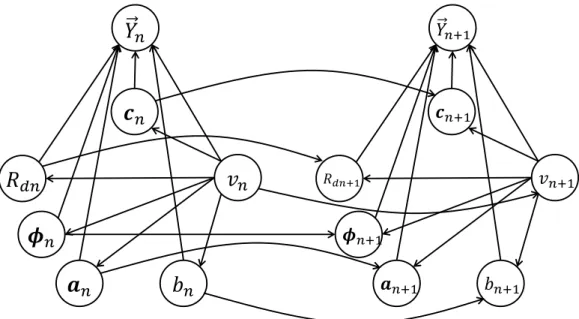
To sum up, the observed variables are {Y~n}. The hidden variables are {vn, b2n,cn, Rdn,an,φn}. Equations (3.6), (3.7), and (3.14) define the obser-vation likelihood conditional on hidden variables. Equations (3.15), (3.16), (3.17), (3.18), (3.19) and (3.20) define the hidden variable priors. Parame-ters are {ρk}2k=0, η, σ2. σb2, µb0, σb20, σ2h, σh20, µg0, σg2, σg20, lg, ug, σa2, σa20,
κ2φ and κ2φ0. Figure 3.1 shows the graphical model of PAT, where each node represents a random variable/vector, and each edge denotes a probabilistic dependence.
𝑌
𝑛𝒄
𝑛𝑣
𝑛𝒂
𝑛𝝓
𝑛𝑅
𝑑𝑛𝑏
𝑛 𝑌𝑛+1 𝒄𝑛+1 𝑣𝑛+1 𝒂𝑛+1 𝝓𝑛+1 𝑅𝑑𝑛+1 𝑏𝑛+13.4
Monte-Carlo Inference
A central problem of applying PAT to various speech processing tasks is how to infer the hidden variables,{vn, b2n,cn, Rdn,an,φn}, from the observed speech frames {Y~n}. The challenge is that the joint probability of PAT is so sophisticated that it is impossible to have a closed-form solution. Also it is highly non-convex so any numerical inference schemes may easily get trapped in local optima.
In this chapter, we propose a carefully designed inference scheme that is based on Markov Chain Monte Carlo (MCMC) [101] and parallel tempering [102].
3.4.1
General MCMC Framework
For notational ease, denote zn as the supervector containing all the hidden variables at frame n. The colon operator zn1:n2 denotes a collection of zn
from n1 to n2. Finally, define
z =z1:N, Y~ =Y~1:N, ~s=~s1:N
MCMC solves the following problem: given a distribution up to an un-known constant,c·pZ, estimate the moment, E(f(Z)). PAT inference falls in this category. Formally, PAT inference evaluates Ehz|Y~i or Eh~s|Y~i under the PDF pz
ζ|Y~, which is only known up to a constant because
pz ζ|Y~= pz(ζ)pY~ ~ Y|z =ζ R pz(ζ0)pY~ ~ Y|z =ζ0dζ0 (3.22)
While the numerator can be evaluated, the denominator is impossible to compute. Instead, MCMC generates a set of samples following the target distribution in a recursive manner. Define z(m) as the m-th sample
gener-ated. Then MCMC generates the next sample based on the current sample, following a transition probability, or transition kernel, Ψ z(m+1)|z(m), which is designed such that the stationary distribution is the target distribution. Different MCMC algorithms differ in the design of transition kernels.
3.4.2
The MH Algorithm and Gibbs Sampler
The MH (Metropolis-Hastings) algorithm [80, 81] is one of the most pop-ular MCMC algorithms, and also the basic building block of our designed algorithm. Algorithm 3.1 shows the typical iteration step of generating a new sample based on the old one. Essentially, it first proposes a new sample with some proposal distributionqz(·|z(m)), and then accepts it with a certain
probability.
Algorithm 3.1 New sample generation step of the MH algorithm
Input: Previous samplez(m), unnormalized target distributionpz,~Y Output: Next sample z(m+1)
Samplez∗ fromqz(·|z(m)) Sampleu from U[0,1] Compute A(z∗,z(m)) = min ( 1, pz,~Y(z ∗, ~Y)q z(z(m)|z∗) pz,~Y(z(m), ~Y)q z(z∗|z(m)) ) (3.23) if u <A(z∗,z(m)) then z(m+1) =z∗ else z(m+1) =z(m) end if
It can be shown that the stationary distribution of the transition kernel introduced in algorithm 3.1 is pz(·|Y~).
A(z∗,z(m)), called the acceptance rate, specifies the probability that the
proposed sample is accepted. It is immediately obvious that the design of proposalqz(·|z(m)) is the key to a successful MH algorithm. A poor proposal
distribution will result in low A(z∗,z(m)) and hence the Markov chain be-comes stagnant. The ideal proposal would be pz(·|Y~) itself, which results in
A(z∗,z(m)) = 1, but obviously this is infeasible.
The Gibbs sampler [82] is a special MH scheme that has acceptance rate one. It updates one dimension of z at a time. Suppose the update order is from z1 (frame 1) to zN (frame N), and within a particular frame zn from dimension 1 to dimension I, which denotes the length of zn, then the proposal distribution of dimension i of zn, denoted as zni, can be expressed
as qzni(·|z (m+1) ni− ,z (m) ni+) =pzni(·|zni− =z (m+1) ni− ,zni+ =zni(m+), ~Y) (3.24)
wherezni−denotes dimensions that are updated beforezni, andzni+denotes
dimensions that are updated after zni. Formally
zni− ={zνι:ν < n∨(ν =n∧ι < i)} zni+ ={zνι:ν > n∨(ν =n∧ι > i)}
Since it can be proved that the acceptance rate is one, the proposed will be always accepted after proposed. After all dimensions are updated, the new sample is generated. Algorithm 3.2 shows a typical updating step of the Gibbs sampler.
Algorithm 3.2 New sample generation step of the Gibbs sampler
Input: Previous samplez(m), unnormalized target distributionp z,~Y
Output: Next sample z(m+1)
for n = 1 :N do for i= 1 : I do Samplezni(m+1) frompzni(·|zni− =z (m+1) ni− ,zni+ =z (m) ni+, ~Y) end for end for
Unfortunately, the Gibbs sampler is still infeasible for PAT. This is be-cause pzni(·|zni− =z
(m+1)
ni− ,zni+ =z (m)
ni+, ~Y) is known only up to an unknown
constant. Even it is completely known, it may be too complex a distribution to numerically draw a sample from. In the next subsection, we will introduce a compromise that is feasible and still retains the good property of the Gibbs sampler in avoiding stagnant Markov chains.
3.4.3
Taylor Expansion Assisted MH
Simplify the Gibbs proposal probability (equation (3.24)) by the Markov property: pzni ζ|zni− =z(nim−+1),zni+ =z (m) ni+, ~Y =pzni ζ|z(n−1)i =z (m+1) (n−1)i,zn(1:i−1) =z (m+1) n(1:i−1), zn(i+1:I)=z (m) n(i+1:I),z(n+1)i =z (m) (n+1)i, ~Yn ∝pzni ζ|z(n−1)i =z (m+1) (n−1)i,z(n+1)i =z (m) (n+1)i ·pY~n ~ Yn|zn(1:i−1) =z (m+1) n(1:i−1),zni =ζ,zn(i+1:I) =z (m) n(i+1:I) ≡πni(ζ) (3.25)
where the last line simply introduces a simplified notation.
The basic idea of our proposed algorithm is to approximate the log [πni(ζ)] with a quadratic polynomial using the Taylor expansion [103], so that πni(ζ) can be approximated by a normal distribution up to a constant. In this way, drawing proposed new samples is much easier. Formally
log(πni(ζ)) =z (m) ni + ∂log(πni(ζ)) ∂ζ ζ=z(m)ni ζ−zni(m) + ∂ 2log(π ni(ζ)) 2∂ζ2 ζ=zni(m) ζ−zni(m) 2 +ni(ζ) ≡ˆtni(ζ) +ni(ζ) (3.26)
ni(ζ) should be very small particularly when ζ is close to z
(m)
ni . Our proposed proposal distribution for PAT is then defined as
qzni(ζ|z (m+1) ni− ,z (m) ni ,z (m) ni+)∝exp ˆtni(ζ) 1(ζ ∈supp(zni)∩ Zni) (3.27) where supp(·) denotes the support of a random variable. Zni denotes an interval around zni(m), within which the Taylor approximation error is reason-ably small. We will formally define and compute Zni later. Notice that the proposal distribution in equation (3.27) is dependent onz(nim), because Taylor expansion is performed around it. This is different from the case in equation (3.24).
The proposal distribution in equation (3.27) is a truncated normal distri-bution, from which it is easy to draw samples. Also, since it is close to the Gibbs proposal distribution, the acceptance rate should be close to one, if not equal to.
Now, we will compute the acceptance rateA(zni∗ ,zni(m)) according to equa-tion (3.23). The notaequa-tion is slightly adapted from equaequa-tion (3.23) because each dimension is separately proposed and the acceptance rate is evaluated for each specific dimension.
A(zni∗ ,z(nim)) = min ( 1, πni(z ∗ ni)qzni(z (m) ni |z (m+1) ni− ,z ∗ ni,z (m) ni+) πni(zni(m))qzni(z ∗ ni|z (m+1) ni− ,z (m) ni ,z (m) ni+) ) = min 1,exp ˆ tni(zni∗ ) +ni(zni∗ ) qzni(z (m) ni |z (m+1) ni− ,z∗ni,z (m) ni+) exphˆtni(z (m) ni ) +ni(z (m) ni ) i expˆtni(zni∗ ) (3.28) To proceed, we need to make an approximation. First note that
qzni
ζ|zni(m−+1),zni∗ ,z(nim+)6=qzni
ζ|zni(m−+1),zni(m),z(nim+)
because Taylor expansion is around a different point zni∗ , and will yield a different polynomial function. However, we can assume thatZniis reasonably small and zni∗ is so close to z(nim+) that the two Taylor expansions are almost the same. Namely
qzni
ζ|z(nim−+1),zni∗ ,zni(m+)≈qzni
ζ|zni(m−+1),zni(m),zni(m+) (3.29) Therefore, according to equation (3.27),
A(z∗ni,zni(m))≈A(ˆ zni∗ ,zni(m)) = min 1, πni(z∗ni) exp h ˆ tni(zni(m)) i πni(z (m) ni ) exp ˆ tni(zni∗ ) = min 1, expˆtni(zni∗ ) +ni(zni∗ ) exp h ˆ tni(z (m) ni ) i exphtˆni(z (m) ni ) +ni(z (m) ni ) i expˆtni(zni∗ ) = minn1,exphni(zni∗ )−ni(z (m) ni ) io (3.30)
(3.30) shows, ifni(zni∗ )−ni(z
(m)
ni ) is sufficiently small, then acceptance rate will be close to one.
ˆ
A(zni∗ ,z(nim)) is not only theoretically meaningful. During implementation, ˆ
A(zni∗ ,zni(m)) will be evaluated instead ofA(zni∗ ,zni(m)), because the former per-forms the Taylor expansion only once and reduces computational complexity significantly.
Now that we know how the Taylor approximation error is related to the acceptance rate, we can use this relation to guide the choice of Zni. Suppose we want
ˆ
A(z∗ni,zni(m))≥1−δ (3.31) Then from the last line in equation (3.30),
ni(zni∗ )−ni(z
(m)
ni )≥log(1−δ)≈ −δ (3.32) A sufficient condition to equation (3.32) is
|ni(ζ)| ≤δ/2 (3.33)
Note from equation (3.26) that ni(ζ) is the residual term of the second-order Taylor expansion of logπni(ζ), which can be further expanded by the third-order Taylor expansion:
ni(ζ) = ∂ 3log (π ni(ζ0)) 6∂ζ03 ζ0=z(m) ni (ζ−zni(m))3+o (ζ−zni(m))3 ≈ ∂ 3log (πni(ζ0)) 6∂ζ03 ζ0=z(m) ni (ζ−zni(m))3 (3.34)
Combining equations (3.32) and (3.34), we get Zni = " z(nim)− 3 s 3δ ∂3log (πni(ζ0))/∂ζ03 |ζ0=z(m) ni , z(nim)+ 3 s 3δ ∂3log (π ni(ζ0))/∂ζ 03 |ζ0=z(m) ni # (3.35)
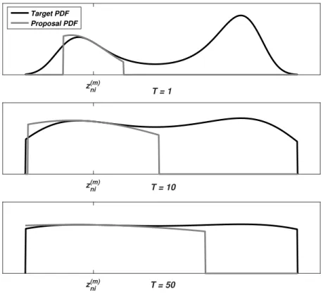
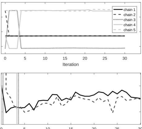
As a summary, the proposed MCMC algorithm is listed in algorithm 3.3. The upper panel of figure 3.2 demonstrates the proposed MH algorithm. The black line denotes the target distribution πni(ζ). The grey line denotes