Structural Reforms in the EU: A simulation-based analysis using the QUEST model with endogenous growth

St

r

uct

ur

al

Ref

or

ms

i

n

t

he

EU:

A

s

i

mul

at

i

on-

bas

ed

anal

ys

i

s

us

i

ng

t

he

QUEST

model

wi

t

h

endogenous

gr

owt

h

Wer

ner

Roeger

,

Janos

Var

ga

and

Jan

i

n

'

t

Vel

d

Economi

c

Paper

s

351|

December

2008

EUROPEAN

ECONOMY

Economic Papers are written by the Staff of the Directorate-General for Economic and Financial Affairs, or by experts working in association with them. The Papers are intended to increase awareness of the technical work being done by staff and to seek comments and suggestions for further analysis. The views expressed are the author’s alone and do not necessarily correspond to those of the European Commission. Comments and enquiries should be addressed to:

European Commission

Directorate-General for Economic and Financial Affairs Publications

B-1049 Brussels Belgium

E-mail: [email protected]

This paper exists in English only and can be downloaded from the website

http://ec.europa.eu/economy_finance/publications

A great deal of additional information is available on the Internet. It can be accessed through the Europa server (http://europa.eu )

Structural Reforms in the EU:

A simulation-based analysis using the QUEST

model with endogenous growth

by

Werner Roeger, Janos Varga and Jan in 't Veld European Commission, DG ECFIN

B-1049 Brussels, Belgium e-mail: [email protected]; [email protected]; [email protected] 18 November 2008 Abstract:

This paper describes a micro-founded DSGE model with endogenous growth that is used to analyse the macroeconomic impact of structural reforms in Europe. The new QUEST III model is a useful tool for analysing the costs and benefits of reforms in terms of concrete and quantifiable policy measures, in particular fiscal policy instruments such as taxes, benefits, subsidies and education expenditures, administrative costs faced by firms and regulatory indices. Our results confirm the beneficial effects on output and employment of skill-biased tax reforms, measures that improve the skill composition of the labour force, R&D subsidies, raising competition in final goods market, increased financial market integration and measures that remove entry barriers in certain markets. The model also allows us to examine the adjustment path and the time lags involved before these benefits can be reaped.

JEL Classification: E32, E62, O30, O41

Keywords: Structural reforms, endogenous growth, R&D, DSGE modelling.

_____________________

The views expressed in this paper are those of the authors and should not be attributed to the European Commission.

Executive Summary

The launch of the Lisbon Strategy in 2000 has started a lively debate on how to best design a strategy to achieve both higher growth and more employment and there has been a related discussion on how to best evaluate structural measures which have an impact on goods, labour and financial markets.

It is widely recognised by now that knowledge investment is a key to economic growth and there is a link between the growth rate of technical progress and knowledge investment, both in the form of higher R&D spending or increased education expenditure. For example, the OECD (2003) estimates that increasing R&D by 0.1% points could increase GDP by about 1.2%, while Fuente (2003) estimates that one year of additional education could raise GDP in the EU by 4 to 6%. However, it is also evident that it is not in the power of governments to increase R&D spending (of the private sector) directly. Instead one has to think about appropriate policies which induce firms to increase intangible investment. These can take a variety of forms, e. g. tax incentives, changes in market structure, supporting public R&D efforts, increasing the pool of qualified R&D personnel etc.

This paper proposes to use a Dynamic Stochastic General Equilibrium (DSGE) model which captures both investment in tangibles and intangibles (R&D), and which also disaggregates employment into various skill categories, as a tool for analysing the effects of particular policy measures. The framework that we adopt is the Jones (1995, 2005) extension of the Romer (1990) endogenous growth model, which uses a variety approach for modelling knowledge investment. DSGE models are particularly well-suited for this task since they capture nominal and real rigidities in goods and labour markets by modelling these markets as imperfectly competitive. This also allows us to look at competition-enhancing policies. The model set up in this paper is sufficiently detailed to be able to address the main reform areas that are discussed within the EU's comprehensive strategy of structural reforms. More specifically we use the model to analyse the following reforms: increasing the employment of low-skilled workers, changing the skill composition of the labour force, fiscal measures for increasing knowledge investment, removing entry barriers and administrative burdens in certain markets and addressing financial market imperfections. Our aim is to explicitly model the reforms in terms of concrete and quantifiable policy measures, in particular fiscal policy instruments such as taxes, benefits, subsidies and education expenditures, administrative costs faced by firms (for both entrants and incumbents) and regulatory indices. For each policy measure a comprehensive set of macroeconomic indicators is presented, showing how particular reforms impact on growth, employment, the composition of investment and skill premia in the short, medium and long run, thus providing insights into the transmission mechanisms of various structural and fiscal measures.

The model has been used to analyse selected structural policies published in the Annual Progress Report of the Commission and is currently used to analyse policies as put forward in the recent Communication from the Commission proposing a European Economic Recovery Plan in response to the financial crisis. The model feeds into the policy making process as a tool which can be used to assess concrete policy initiatives designed to counter adverse effects of the financial crisis concerning their short, medium and long run growth and employment impacts.

Introduction

Designing policies to foster economic growth and job creation in the European Union is one of the principal goals of the Lisbon Strategy for Growth and Jobs. Since the initiation of the Lisbon Strategy in 2000 there has been a lively debate on how to best design a strategy to achieve both higher growth and more employment. This has become even more critical in the recent financial crisis which is expected not only to lower actual growth but also to reduce the potential growth rate in the medium term1. However, as emphasised in a review of Lisbon related research the Commission (European Commission, 2005) states: "…at this stage we have only a partial view of the impact of specific reforms and we not yet fully understand the interactions between the different reforms envisaged in the Lisbon Strategy." Also Sapir (2007) points out that there are large deficiencies in the methodology to evaluate structural reforms. In particular he stresses that structural reforms are essentially microeconomic policy measures, which implies that without a clear view on how particular measures affect goods, labour and financial markets it will be difficult to assess their impact on growth and employment. Sapir (2007) states in this context: "…using a macro-model to assess the impact of structural reforms requires a careful modelling of the intermediate microeconomic effects." This poses a challenge to model builders. In this paper we want to make a step in the direction of dealing with this challenge.

Standard modern macro-economic models, so called Dynamic Stochastic General Equilibrium (DSGE) models, go some way in the direction of meeting the requirement of micro foundations and also typically model imperfections in goods and labour markets. DSGE models try to capture nominal and real rigidities in goods and labour markets by modelling these markets as imperfectly competitive. Nevertheless, standard models still lack sufficient detail to make a direct link between concrete reform efforts and market outcomes. For example it is typical in macro studies of the impact of structural reforms to analyse reforms by giving shocks to mark-ups and TFP (see for example Bayoumi et al. (2004) and studies based on CGE models). Such exercises are certainly useful if one is interested in understanding productivity and employment differences between two countries with different levels of mark-ups and TFP. However, it is less useful in a policy context as long as one cannot link these variables to policy measures. Another weak point of existing macro models is that they are not detailed enough to address specific policy areas. This becomes immediately clear when one looks at the main reform areas. For example, the employment rate in Europe differs significantly across skill groups. Therefore a policy of increasing the employment rate must devise measures to increase the demand and supply of low skilled workers or change the composition of the labour force. Analysing labour market policies therefore requires a disaggregation of the labour market, which is not a common practice in macro models. One of the most prominent Lisbon targets is to increase R&D expenditure to 3% of GDP. It is widely recognised by now that knowledge investment is a key to economic growth and there is a link between the growth rate of technical progress and R&D spending. However, it is also clear that it is not in the power of governments to increase R&D spending (of the private sector) directly but one has to think about appropriate policies which induce firms to increase intangible investment. These can take a variety of forms, e. g. tax incentives, changes in market structure, supporting public R&D efforts, increasing the pool of qualified R&D personnel etc.. What is required is a disaggregation of investment into tangibles and

1 _{In response to the financial crisis, the Commission is proposing a detailed EU recovery framework, under the}

umbrella of the Lisbon strategy for growth and jobs, bringing together a series of targeted short term initiatives designed to help counter adverse effects of the financial crisis on the wider economy and adapting the medium to long term measures of the Lisbon strategy to take account of the crisis.

intangibles which is not standard practice in macro models. Such a disaggregation is conceptually much more demanding then for example skill disaggregation of the labour force, because these two types of goods have fundamentally different economic characteristics. Physical capital is a conventional good. Basically this means two things. First, the use of a piece of fixed capital by one firm precludes its use by another firm, i.e. it is rivalrous. Second, the quantity of output produced can be modelled within a standard production function framework with constant returns-to-scale. Knowledge capital is different in both dimensions. It usually comes in the form of a design for the production of a new good. In contrast to physical capital it is non-rivalrous (see Romer,1990), i.e. a firm which is in the possession of a new design cannot automatically preclude other firms from using it and there can be knowledge spillovers. Also, once a design has been created it can be used in production for as large a quantity as is required by the market without duplicating the design. Thus knowledge capital takes the form of a sunk cost for the firm and production becomes increasing returns-to-scale. This not only has technological implications but also has consequences for market structures which are compatible with this technology. Endogenous growth models as pioneered by Romer (1990), and further developed by Jones (1995) and Aghion and Howitt (1998), provide the conceptual framework to deal with these issues. This is also the framework we use in this paper. As implied by these models, striking an adequate balance between efficiency and competition becomes a complex issue.

In this paper we make an attempt to set up a model that is sufficiently detailed to be able to address the main reform areas that are discussed within the EU's comprehensive strategy of structural reforms. More specifically we use the model to analyse the following reforms: increasing the employment of low-skilled workers, changing the skill composition of the labour force, increasing knowledge investment, removing entry barriers in certain markets and addressing financial market imperfections. Our aim is to explicitly model the reforms in terms of concrete and quantifiable policy measures, in particular fiscal policy instruments such as taxes, benefits, subsidies and education expenditures, administrative costs faced by firms (for both entrants and incumbents) and regulatory indices. This makes the model a useful tool for analysing the costs and benefits of structural reforms, but it can also be usefully applied to address questions concerning the quality of public finances.

The model we use in this paper is an extension of the QUEST III model with endogenous growth. The new QUEST III model is a global DSGE model employed in the Directorate-General Economic and Financial Affairs of the European Commission for quantitative policy analysis. This model belongs to the new class of micro-founded DSGE models that are now widely used in economic policy institutions2. Equations in these models are explicitly derived from intertemporal optimisation under technological, institutional and budgetary constraints and the model incorporates nominal, real and financial frictions in order to fit the data (Ratto et al., 2008). The model employs the product variety framework proposed by Dixit and Stiglitz (1977) and applies the Jones (1995) semi-endogenous growth framework to explicitly model the underlying development of R&D.

Our paper can be compared to Bayoumi et al. (2004), which uses the IMF's Global Economy Model GEM to analyse the macroeconomic benefits from increasing competition in euro area labour and product markets to US levels. Based on empirically estimated mark-ups for the euro area and the US, they find that lowering price and wage mark-ups to US levels could raise output per capita by about 12 ½ percent and close about half the observed per-capita

2 _{See for example the International Monetary Fund's Global Economy Model (Bayoumi et al., 2004) and the}

output gap between the two regions. Coenen et al. (2007) employ the ECB's New Area-Wide Model NAWM to examine the effects of reducing the euro area tax wedge to levels prevailing in the US and find that this would result in an increase in hours worked and output of more than 10 percent. In our paper we investigate a wider range of policies and we use an endogenous growth framework3. We find that the effect of reducing price mark-ups is not unambiguous and depends on the sector in which it occurs. In our intermediate goods sector mark-ups cover the costs associated with acquiring a patent when entering the market, and reducing mark-ups can have a detrimental impact on growth and employment if it reduces entry of new firms. Concerning tax reforms, Coenen et al. consider reductions in the overall tax burden that are offset by changes in government transfers to households, while we look at the effects of a shift in the tax burden from labour tax to consumption tax.

The paper is organised as follows. Section 1 contains a detailed description of the model. Section 2 discusses calibration and estimation of structural parameters. Section 3 then shows the properties of the model by presenting various reform scenarios. The final section concludes.

1 Model

The model economy is populated by households, final and intermediate goods producing firms, a research industry, a monetary and a fiscal authority4. In the final goods sector firms produce differentiated goods which are imperfect substitutes for goods produced abroad. Final good producers use a composite of domestic and imported intermediate goods and three types of labour - (low-, medium-, and high-skilled). Households buy the patents of designs produced by the R&D sector and license them to the intermediate goods producing firms. The intermediate sector is composed of monopolistically competitive firms which produce intermediate products from rented capital input using the designs licensed from the household sector. The production of new designs takes place in research labs, employing high skilled labour and making use of the existing stock of domestic and foreign ideas. Technological change is modelled as increasing product variety in the tradition of Dixit and Stiglitz (1977). 1.1 Households

The household sector consists of a continuum of households . A share (1-ε) of these households are not liquidity constrained and indexed by

[

0,1

∈

h

[

0,1−ε

]

]

∈

i . They have access to financial markets where they can buy and sell domestic and foreign assets (government bonds), accumulate physical capital which they rent out to the intermediate sector, and they also buy the patents of designs produced by the R&D sector and license them to the intermediate goods producing firms. Non-liquidity constrained household members offer

3 _{In another paper (Roeger et al., 2008) we use the model to identify possible sources for the productivity gap}

between the EU and the US and look at policies which could help to close this gap. The framework allows us to explain differences in productivity and R&D spending levels in terms of differences in taxation, subsidies to R&D, mark ups in labour and goods markets, entry barriers, efficiency of the R&D sector and the skill composition of the labour force.

4 _{The model can be used in a one-country, open-economy version and it can also be extended to more regions}

(e.g. Euro Area and non Euro Area blocks of the EU, US, Asia, major oil-exporters). Individual European Union member states can also be modelled separately in interaction with the rest of the EU.

medium- and high-skilled labour services indexed by . The remaining share ε of households is liquidity constrained and indexed by

{

M H s∈ ,

[

1 ,1

}

]

ε − ∈ k i t J ucap

. These households cannot trade in financial and physical assets and consume their disposable income each period. Members of liquidity constrained households offer low-skilled labour services only. For each skill group we assume that both types of households supply differentiated labour services to unions which act as wage setters in monopolistically competitive labour markets. The unions pool wage income and distribute it in equal proportions among their members. Nominal rigidity in wage setting is introduced by assuming that households face adjustment costs for changing wages.

1.1.1 Non liquidity constrained households

Each non liquidity constrained household maximise an intertemporal utility function in consumption and leisure subject to a budget constraint. These households makes decisions about consumption ( ), labour supply ( ), investments into domestic and foreign financial assets ( and ), the purchases of investment good ( ), the renting of physical capital stock ( ), the corresponding degree of capacity utilisation ( ), the purchases of new patents from the R&D sector ( ), and the licensing of existing patents ( ), and receives wage income ( ), unemployment benefits ( )

i t C i t L i t B i t K i F t B , i t W i t i A t J , K t i , i t A s i t s tW

b , 5_{, transfer income from the government}

( ) ,and interest income (i ). Hence, non-liquidity constrained households face the following Lagrangian

i t TR A t t andi

5 _{Notice, households only make a decision about the level of employment but there is no distinction on the part}

of households between unemployment and non participation. It is assumed that the government makes a decision how to classify the nonworking part of the population into unemployed and nonparticipants. The non

-participation rate NPART must therefore be seen as a policy variable characterising the generosity of the benefit system.

(1)

(

)

(

)

(

(

)

)

(

)

(

)

(

)

(

i

)

t A i A t i t t t i t i t i t K i t i t t t i t i t t A j i x t j n j i f t j i t i A t A t A i t A t A K t i t A t A t A t K t i t I t K i t I t K K t i t J t i t U K t i t K t K t s s i t W s i t s i t s i t s t s i t s i t s w t i F t t t F t t B F t i t t i A t A t i t J i t I t i F t t i t i t C t c t t i t t s s i t i t t i ucap A J K J B B L C A J A K J K PR PR TR J P A P t A P rp i t J P K P t K P ucap rp ucap i t W L NPART W b L W t B E Y B E r B r J P J J P B E B C P t L V C U V Max t F t i t i t i A t i t i t i F t i t i t i t 1 , 0 0 1 0 0 0 1 , , 1 , , , 1 1 1 1 1 1 1 1 1 1 1 1 1 1 , , , , , , , , 1 1 1 1 1 1 , , 0 0 , 0 0 , , , , , , ) 1 ( ) 1 ( ) )( 1 ( ) 1 ( ) ( ) 1 ( 1 / 1 1 ) ( ) 1 ( ) 1 ( ) ( 0 , , − ∞ = − ∞ = ∞ = = = − − − − − − − − − − − − − − ⎟ ⎠ ⎞ ⎜ ⎝ ⎛ − − − − − − ∞ = ⎪ ⎭ ⎪ ⎬ ⎫ ⎪ ⎩ ⎪ ⎨ ⎧ − − − Ε − − − − Ε − ⎟⎟ ⎟ ⎟ ⎟ ⎟ ⎟ ⎟ ⎟ ⎟ ⎟ ⎠ ⎞ ⎜⎜ ⎜ ⎜ ⎜ ⎜ ⎜ ⎜ ⎜ ⎜ ⎜ ⎝ ⎛ − − − − − − − − − − Γ − − − − Γ + − − − − − Γ − + − + − + Γ + + + + + Ε − ⎟⎟ ⎠ ⎞ ⎜⎜ ⎝ ⎛ − + Ε =

∑

∑

∑

∑

∑

∑

∑

∑

∞ = δ β ψ λ δ β ξ λ τ δ τ δ β λ β } , {M H s∈

The budget constraints are written in real terms with all prices and wages normalized with Pt,

the price of domestic final goods. All firms of the economy are owned by non liquidity constrained households who share the total profit of the final and intermediate sector firms, and , where n and At denote the number of firms in the final and

intermediate sector respectively. As shown by the budget constraints, all households pay wage income taxes and capital income taxes less tax credits (_τK _{and τ}A_{) and depreciation}

allowances ( _δK and A) after their earnings on physical capital and patents. There is no perfect arbitrage between different types of assets. When taking a position in the international bond market, households face a financial intermediation premium

∑

= n j i f t j PR 1 , ,

∑

₌ t A j i x t j PR 1 , , K t t K t t _δ w t t K t t (.) F B Γ which depends on the economy-wide net holdings of internationally traded bonds. Also, when investing into tangible and intangible capital households require premia and in order to cover the increased risk on the return related to these assets. The real interest rate rt is equal to the

nominal interest rate minus expected inflation:

K t rp ) ( _t+1 A t rp − = t t t i E r _π .

The utility function is additively separable in consumption ( ) and leisure ( ). We assume log-utility for consumption and allow for habit persistence.

i t C is t L, 1− (2a) ( )=(1− )log

(

− t₋₁

)

. i t i t habc C habcC C U

For leisure we assume CES preferences with common labour supply elasticity but a skill specific weight (_ωs) on leisure. This is necessary in order to capture differences in employment levels across skill groups. Thus preferences for leisure are given by

(2b) (1 ) , 1 ) 1 ( , , 1 κ κ ω ₋ − − = − is t s s i t L L V with κ >0.

The investment decisions w.r.t. real capital and decisions w.r.t. the degree of capacity utilisation are subject to convex adjustment costs Γ_J and Γ_U, which are given by

(3a)

( )

2 1 2 ) ( 2 2 ) ( i t I i t i t K i t J J K J J = + Δ Γ − γ γ _and (3b) ( ) ₁

(

) (

₂ ss

)

2 , t i t ss t i t i t

U ucap =a ucap −ucap +a ucap −ucap

Γ

where ss is the steady state capacity utilisation.

t

ucap

Wages are also subject to convex adjustment costs given by

(4)

∑

− Δ = Γ s tis s i t s i t W s i t W W W L W _, 1 2 , , , 2 ) ( γ

Consumption (C) and investment (J) is itself an aggregate of domestic and foreign varieties of final goods, with preferences expressed by the following CES utility function

(5a) ( 1) 1 1 1 1 ) 1 ( − − − ⎥ ⎥ ⎦ ⎤ ⎢ ⎢ ⎣ ⎡ + − = σ σ σ σ σ σ σ σ di M fi M i _{s Z s Z} Z

with _Zi_∈

{

_Ci_,Ii

}

and _Zdi _{and Z}fi _{are indexes of demand across the continuum of}

differentiated goods produced respectively in the domestic economy and abroad, given by

(5b) 1 1 1 1 1 − = − ⎥ ⎥ ⎦ ⎤ ⎢ ⎢ ⎣ ⎡ ⎟ ⎠ ⎞ ⎜ ⎝ ⎛ =

∑

d d d d d d m h i d h d i d _Z m Z σ σ σ σ σ , 1 1 1 1 1 − = − ⎥ ⎥ ⎦ ⎤ ⎢ ⎢ ⎣ ⎡ ⎟ ⎠ ⎞ ⎜ ⎝ ⎛ =

∑

m m f m m m m h i f h f i f _Z m Z σ σ σ σ σ .

We denote with _PC _{the corresponding utility based deflator for the C and J aggregate. The}

first order conditions of the household with respect to consumption, financial and real assets are given by the following equations:

(6a) 0 _{=> , −} (1₊ ) ₌0, ∂ ∂ C t c t i t i t C i t P t U C V λ (6b) 0 _{=>− +Ε}

(

₁

(

1₊

)

)

₌0, ∂ ∂ + t i t t i t i t r B V β λ λ (6c) 0_{, =>− +Ε}

(

₁

(

1_{+ −Γ}

(

/

)

)

₁/

)

₌0 ∂ ∂ + + t t t F t t B F t i t t i t i F t E E Y B E r B V F β λ λ

(6d)

(

)

(

)

(

)

(

_{1 1} (1 ) ₁ (1 ) ₁

)

0 0 _{=>− +Ε − + − − −Γ + =} ∂ ∂ + + + + tC K K t i t u K t i t K t K t i t i t i t t i t i t i t P t ucap rp ucap i t K V δ β λ δ β ξ λ ξ λ (6e) 1

(

_{1 1 1}

)

0 1 0 _{+ Δ + =} ⎟ ⎟ ⎠ ⎞ ⎜ ⎜ ⎝ ⎛ − Δ + ⎟⎟ ⎠ ⎞ ⎜⎜ ⎝ ⎛ + − => ∂ ∂ + + + − i t i t i t I C t i t t K i t I i t i t K C t i t i t J P E J K J P J V ξ λ γ β λ τ γ γ λ (6f) 0 _{=> − 1−}2 ₂

(

₋

)

₌0 ∂ ∂ ss t i t K t i t ucap ucap a a i ucap V .

All arbitrage conditions are standard, except for a trading friction (Γ_BF(.)) on foreign bonds, which is modelled as a function of the ratio of assets to GDP. Using the arbitrage conditions and neglecting the second order terms, investment is given as a function of the variable Q_t

(7a) _⎟⎟ ⎠ ⎞ ⎜⎜ ⎝ ⎛ − + Δ − − Δ + ⎟⎟ ⎠ ⎞ ⎜⎜ ⎝ ⎛ = − + + − t tC i t I t K i t I i t i t K t i J E J K J Q 1 1 1 1 1 π γ τ γ γ with _C t t t P Q = ξ ,

where is the present discounted value of the rental rate of return from investing in real assets t Q (7b)

(

(

)

)

_⎟⎟ ⎠ ⎞ ⎜⎜ ⎝ ⎛ − + + Γ − − − + − + − Ε = + + + t tC K K t i t u K t i t K t K t t C t t t t i t ucap rp ucap i t Q i Q 1 1 1 1 ) 1 ( 1 1 π δ π δ

Notice, the relevant discount factor for the investor is the nominal interest rate adjusted by the trading friction minus the expected inflation of investment goods ( C ).

t+1

π

Non-liquidity constrained households buy new patents of designs produced by the R&D sector ( ) and rent their total stock of design ( ) at rental rate to intermediate goods producers in period t. Households pay income tax at rate on the period return of intangibles and they receive tax subsidies at rate τA_{. Hence, the first order conditions with}

respect to R&D investments are given by

A t I A_t A t i K t t (7c) 0 _{=>− +Ε}

(

_{1 1} (1₋ )_{+ 1}

(

(1₋ )( ₋ )₊

)

₁

)

₌0 ∂ ∂ + + + + tA A K t A t A t K t i t A i t i t t i t i t i t P t rp i t A V δ β λ δ β ψ λ ψ λ (7d) 0_{, =>−}

(

1₋

)

_{+ =}0 ∂ ∂ i t i t A A t i t i A t P J V ψ λ τ λ

Therefore the rental rate can be obtained from (6b), (7c) and (7d) after neglecting the second order terms:

(7c')

(

)

A t K t A K t A A t t A A t rp t t i i + − − + − − ≈ + ) 1 ( ) 1 ( _{τ π 1 δ δ} where _A t A t A t P P ₁ 1 1 + + = +π .

Equation (7c') states that household require a rate of return on intangible capital which is equal to the nominal interest rate minus the rate of change of the value of intangible assets and also covers the cost of economic depreciation plus a risk premium. Governments can affect investment decisions in intangible capital by giving tax incentives in the form of tax credits and depreciation allowances or by lowering the tax on the return from patents.

1.1.2 Liquidity constrained households

Liquidity constrained households do not optimize but simply consume their current income at each date. Real consumption of household k is thus determined by the net wage income plus net transfers (8)

(

)

k t s s k t s k t s k t s t s k t s k t s w t s _tks s k t s k t W k t C t c t t W L b W NPART L TR W W L C P t ⎟ + + ⎠ ⎞ ⎜ ⎝ ⎛ − ∑ ∑ Δ = − − − + + 1 (1 ) 2 ) 1 ( , , , , , , , 1 2 , , γ . 1.1.3 Wage setting

Within each skill group a variety of labour services are supplied which are imperfect substitutes to each other. Thus trade unions can charge a wage mark-up ( ) over the reservation wage W t η / 1

6_{. The reservation wage is given as the marginal utility of leisure divided by}

the corresponding marginal utility of consumption. The relevant net real wage to which the mark up adjusted reservation wage is equated is the gross wage adjusted for labour taxes, consumption taxes and unemployment benefits which act as a subsidy to leisure. Thus the wage equation is given as

(9) _C t C t s t s w t s t W t h t C s h t L P t b t W U U ) 1 ( ) 1 ( 1 , , , , 1 + − − = − η for h∈{i,k} and s∈{L,M,H}. 1.1.4 Aggregation

The aggregate of any household specific variable h in per capita terms is given by

t

X

6 _{The mark-up depends on the intratemporal elasticity of substitution between different types of labour σ} s and

fluctuations in the mark-up arise because of wage adjustment costs and the fact that a fraction (1-sfw) of workers is indexing the growth rate of wages πw _{to wage inflation in the previous period}

[

w

]

t w t w t s W s w t σ γ σ β sfwπ sfwπ π η =1−1/ − / ( ₊₁ −(1− ) ₋₁)−

(10)

(

1

)

, 1 0 k t i t h t t X dh X X X =

∫

= −_ε +_ε

Hence aggregate consumption and employment is given by

(11)

(

)

k t i t t C C C = 1−_ε +_ε and (12)

(

1

)

k. t i t t L L L = −_ε +_ε 1.2 Firms

1.2.1 Final output producers

Since each firm j ( ) produces a variety of the domestic good which is an imperfect substitute for the varieties produced by other firms it acts as a monopolistic competitor facing a demand function with a price elasticity given by . Final output (

n j ₌1,....,

d

σ _Yj_{) is produced using A}

varieties of intermediate inputs (x) with an elasticity of substitution _θ. The final good sector uses a labour aggregate and domestic intermediate goods with Cobb-Douglas technology, subject to a fixed cost FCY and overhead labour FCL

(13)

(

(

)

)

( )

j θ _Y t i A i L j t Y, exog t j _{A L FC x FC} Y t _⎟⎟ − ⎠ ⎞ ⎜⎜ ⎝ ⎛ − = − =

∑

θ α α 1 , 1 , 0 < _θ < 1 with (14)

(

)

(

)

(

)

1. 1 1 1 1 1 1 , , − − − − ⎟ ⎠ ⎞ ⎜ ⎝ ⎛ _{+ +} = L L L L L L L L L L L HY t H Y H M t M M L t L L t Y s ef L s ef L s ef L L σ σ σ σ σ σ σ σ σ σ σ

Parameter ss is the population share of labour-force in subgroup s (low-, medium- and

high-skilled), Ls denotes the employment rate of population s, efs is the corresponding efficiency

unit, and _σL is the elasticity of substitution between different labour types. Note that high-skilled labour in the final goods sector, , is the total high-skill employment minus the high-skilled labour working for the R&D sector ( ). The employment aggregates combine varieties of differentiated labour services supplied by individual household

HY t L t A L _, s t L (15) 1 1 0 1 , − − ⎥ ⎦ ⎤ ⎢ ⎣ ⎡ = ∫ s s s s dh L L sh t s t σ σ σ σ

The parameter σs >1 determines the degree of substitutability among different types of labour.

The above production function employs the idea of product variety framework proposed by Dixit and Stiglitz (1977) and applied in the literature of international trade and R&D diffusion7 and we will explicitly model the underlying development of R&D by the semi-endogenous framework of Jones (1995 and 2005)8.

The objective of the firm is to maximise profits

(16)

(

)

j , t i t i A i HY j t H t M j t M t L j t L t j t j t j f t P Y W L W L W L px x PR t , , 1 , , , ,

∑

= − + + − =

(

)

where px is the price of intermediate inputs and is a wage index corresponding to the CES aggregate . All prices and wages are normalized with Pt, the price of domestic final

goods. In a symmetric equilibrium, the demand for labour and intermediate inputs is given by

s t W s j t L , (17a) s ef W s

{

L M H

}

L L FC L FC Y s t t s s s t t Y L t Y Y t L L L L , , , 1 1 1 , , ∈ = ⎟ ⎟ ⎠ ⎞ ⎜ ⎜ ⎝ ⎛ − + − η α σ σ σ σ (17b)

(

) ( ) (

_, 1 1 , 1 , (1 ) − − = ⎟⎟⎠ ⎞ ⎜⎜ ⎝ ⎛ + − =η α

∑

it θ θ j t i A i Y t t t i Y FC x x px t

)

where d 9 t t σ η =1−1/

1.2.2 Intermediate goods producers

The intermediate sector consists of monopolistically competitive firms which have entered the market by licensing a design from domestic households and by making an initial payment to overcome administrative entry barriers. Capital inputs are also rented from the household sector for a rental rate of . Firms which have acquired a design can transform each unit of capital into a single unit of an intermediate input. Intermediate goods producing firms sell their products to domestic final good producers. In symmetric equilibrium the inverse demand function of domestic final good producers is given as equation (17b).

A

FC

K t

i

Each domestic intermediate firm solves the following profit-maximisation problem

(18)

{

A _A

}

t A t i C t K t t i t i x x t i px x i P k i P FC PR t i − − − = , , , , , max

7 _{See Grossman and Helpman (1991) and Aghion and Howitt (1998).}

8 _{Butler and Pakko (1998) also applied Jones (1995) semi-endogenous growth framework to examine the effect}

of endogenous technological change on the properties of a real business cycle model without skill disaggregation.

9 _{Similar to the wage mark-up, we allow for fluctuations in the mark-up of prices because of price adjustment}

costs and the fact that a fractionof firms is indexing price increases to inflation in the previous period (see footnote 5).

subject to a linear technology which allows to transform one unit of effective capital (ki·ucapt)

into one unit of an intermediate good (19) x_i,_t =k_i,_t ⋅ucap_t.

In a symmetric equilibrium the first order condition is

(20a)

(

) ( ) ( )

C t K t t θ j t i A i Y t t Y FC x x i P t = ⎟⎟ ⎠ ⎞ ⎜⎜ ⎝ ⎛ + − − − =

∑

1 1 , 1 ) 1 ( _α θ θη

Intermediate goods producers set prices as a mark up over marginal cost. Therefore prices for the domestic market are given by:

(20b) _, . θ C t K t t i t P i px PX = =

The no-arbitrage condition requires that entry into the intermediate goods producing sector takes place until

(21a) PR PR i PA r_tFC_A i t A t x t x t i, = = + , ∀

or equivalently, the present discounted value of profits is equated to the fixed entry costs plus the net value of patents

(21b)

(

)

. 1 1 1 1 1 0 0 x t j t j A A A K t A t PR r FC t P τ _τ τ τ δ + = + ∞ =

∏

∑

_⎟⎟ ⎠ ⎞ ⎜ ⎜ ⎝ ⎛ + = + + − −

For an intermediate producer, entry costs consist of the licensing fee for the design or patent which is a prerequisite of production of innovative intermediate goods and a fixed entry cost . A t A t P i A FC 1.2.3 R&D sector

Innovation corresponds to the discovery of a new variety of producer durables that provides an alternative way of producing the final good. The R&D sector hires high-skilled labour (LA)

and generates new designs according to the following knowledge production function: (22) _ν ϖ φ λ . t A t t t A A L A * _{1 ,} 1 − − = Δ

In this framework we allow for international R&D spillovers following Bottazzi and Peri (2007). Parameters ϖ and _φ measure the foreign and domestic spillover effects from the aggregate international and domestic stock of knowledge (A* and A) respectively. Negative value for these parameters can be interpreted as the "fishing out" effect, i.e. when innovation decreases with the level of knowledge, while positive values refer to the "standing on shoulders" effect and imply positive research spillovers. Note that φ =1 would give back the

strong scale effect feature of fully endogenous growth models with respect to the domestic level of knowledge. Parameter _ν can be interpreted as total factor efficiency of R&D production, while _λ measures the elasticity of R&D production on the number of researchers ( ). The international stock of knowledge grows exogenously at rate . We assume that the R&D sector is operated by a research institute which employs high skilled labour at their market rate . We also assume that the research institute faces an adjustment cost of hiring new employees and maximizes the following discounted profit-stream:

A L g_AW H W (23) ⎟ ⎠ ⎞ ⎜ ⎝ ⎛ A t P Δ − − Δ 2 , 2 max , At H t A H t t LAt A W L W L γ

∑

∞ =0 t t d _A,t

therefore the first order condition implies:

(24) Δ = +

(

Δ _, − ₊₁Δ _,+1

)

, t A H t t t A H t A H t t W dW L P _γ λ t A t A L A L W

where dt is the discount factor.

1.3 Trade and the current account

The economies trade both final and intermediate goods. The elasticity of substitution between bundles of domestic and foreign goods _Zdi _{and Z}fi _{is σ. Thus aggregate imports are given}

by (25) ( _t + _t ) EX t P t IM C t C I G IM _⎟⎟ + ⎠ ⎞σ t t P P ⎜ ⎜ ⎝ ⎛ * t P r + 1 M s = t P = t E = F t =(

And there is producer pricing of imports and exports. (26) P_tEX

and

(27) IM t

P

Thus net foreign assets evolve according to

(28) F _{t t}IM _t. t t F t tB E B EX P IM E ) −1+ − 1.4 Policy

On the expenditure side we assume that government consumption, government transfers and government investment are proportional to GDP and unemployment benefits are indexed to wages as follows

(29) (1 s), t s t s s t s t t b W NPART L BEN =∑ − −

where the benefit replacement rate can be indexed to consumer prices and net wages in different degrees according to the following rule

s t b (30)

[

]

c W w, t C t C t s t s t b t P t b = ˆ (1+ ) χ (1− )χ 0≤_χc,_χw ≤1

The government provides subsidies ( ) on physical capital and R&D investments in the form of a tax-credit and depreciation allowances

t S (31)

(

)

AiH. t A t A H i t I t K H i t A t A H i t I t K K t t t P K P A P J P J S , , ,, 1 , 1 1 δ +δ +τ +τ = _{− − −}

Government revenues are made up of taxes on consumption as well as capital and labour income. Government debt ( ) evolves according to

G t R t B (32) LS t G t t t t t C t t t t r B P G TR BEN S R T B =(1+ ) ₋1 + + + + − − .

There is a lump-sum tax ( ) used for controlling the debt to GDP ratio according to the following rule LS t T (33) _⎟⎟ ⎠ ⎞ ⎜⎜ ⎝ ⎛ Δ + ⎟⎟ ⎠ ⎞ ⎜⎜ ⎝ ⎛ − = Δ − − − t t t DEF T t t t B LS t P Y B b P Y B T _{τ τ} 1 1 1

where _bT is the government debt target.

Monetary policy is modelled via the following Taylor rule, which allows for some smoothness of the interest rate response to the inflation and output gap

(34) INOM t t t t INOM y t INOM y T C t INOM T EQ INOM lag t INOM lag t u ygap ygap ygap r i i + − + + − + + − + = + − − ) ( ] ) ( )[ 1 ( 1 2 , 1 1 , 1 τ τ π π τ π τ τ π

The Central bank has a constant inflation target and it adjusts interest rates whenever actual consumer price inflation deviates from the target and it also responds to the output gap. There is also some inertia in nominal interest rate setting.

T

π

Rather than defining the output gap as the difference between actual and efficient output, we use a measure that closely approximates the standard practice of output gap calculation as used for fiscal surveillance and monetary policy (see Denis et al. (2006)), in which a production function framework is used where the output gap is defined as deviation of capital and labour utilisation from their long run trends. Therefore we define the output gap as

(35) α α ⎟⎟ ⎠ ⎞ ⎜⎜ ⎝ ⎛ ⎟⎟ ⎠ ⎞ ⎜⎜ ⎝ ⎛ = − ss t t ss t t t L L ucap ucap YGAP ) 1 ( .

where and are moving average steady state employment rate and capacity utilisation: ss t L ss t ucap (36) ss ucap _t t ucap ss t ucap ucap ucap =(1−_ρ ) ₋1 +_ρ (37) ss Lss _t t Lss ss t L L L =(1−_ρ ) −1+_ρ

which we restrict to move slowly in response to actual values.

2 Calibration

2.1 Goods Market

We identify the final goods sector as the service sector and the intermediate sector as the manufacturing sector. The manufacturing sector resembles the intermediate sector along various dimensions. First, this sector is more R&D and patent intensive, second, a large fraction of manufacturing supplies innovative goods (in the form of investment goods but also innovative consumer goods). Services on the other hand are typically not subject to large (patented) innovations but are subject to organisational changes possibly in relation to new technologies supplied by the manufacturing sector. A good example in this respect is the ICT investment driven productivity increase in retail, wholesale trade and banking in some countries, notably the US. Also the two sectors differ in the degree of competition, with manufacturing showing smaller mark ups compared to services. For calculating mark ups we use a method suggested by Roeger (1995). We find substantially high mark ups in services in the EU (24%) while mark ups in manufacturing are lower (12%). Similar results but with even stronger differences in manufacturing industries have been obtained by Christopoulou and Vermeulen (2008). The results on cross country differences in the level of mark ups are interesting since they suggest a positive link between the level of mark ups and R&D investment as suggested by our model. This comes out even clearer in earlier work by Oliveira Martins et al. (1996) which shows that sectors with high R&D intensities tend to have higher mark ups.

It is a stylised fact that product markets are more regulated in the EU compared to the US. Recent evidence can be found in Hoj et al. (2007). To our knowledge estimates on entry barriers for specific sectors do not exist. Therefore we rely on the aggregate estimates provided by Djankov et al. (2002). These estimates are particularly useful since they provide directly quantifiable evidence on costs of procedures and time that a start-up must bear before the firm can operate legally. This information can be directly used for the calibration of the entry cost parameter in the model. The average entry cost per firm is estimated to be around 66 percent of GDP per capita in the whole sample. Their calculations show that the European countries impose 2 to 60 times higher entry costs than the US. Based on the Djankov et al. (2002) methodology Kox (2005) re-estimated the start-up costs for the EU. He estimates the EU average entry cost of setting up a standard firm at 57.3 percent of per capita GDP and only to 1.6% for the US. Cross country variation is large and ranges from 4.5 percent of per capita GDP for the UK to 1.83 times per capita GDP in Hungary.

2.2 R&D sector

Empirical evidence on output elasticities of R&D production has recently been provided by Bottazzi and Peri. (2007) 10. Concerning the subsidies to R&D investments, empirical evidence provided by Warda (1996, 2006) indicates an average of 5 percentage point net R&D subsidies for the EU based on the B-index11.

2.3 Labour market

We use information from our estimation of the core QUEST III model (see Ratto et al. (2008)) to calibrate the parameters of the utility function, labour supply elasticity and the frictional parameters. Labour force is disaggregated into three skill-groups: low-, medium- and high-skilled labour12. Data on skill-specific population shares, participation rates and wage-premia are obtained from OECD (2006), the Labour Force Survey and Science and Technology databases of EUROSTAT. The elasticity of substitution between different labour types (σ) is one of the major issue addressed in the labour-economics literature. We follow Caselli and Coleman (2006) which analysed the cross-country differences of the aggregate production function when skilled and unskilled labour are imperfect substitutes. The authors argue in favour of using the Katz and Murphy (1992) estimate of 1.4. We set the efficiency of low-skilled at 1 for EU27, the other efficiency units are restricted by the labour demand equations which imply the following relationship between wages, labour-types and efficiency units: l l l m m l m m ef L s L s w w ef L L L 1 1 1 − − ⎟⎟ ⎠ ⎞ ⎜⎜ ⎝ ⎛ ⎟⎟ ⎠ ⎞ ⎜⎜ ⎝ ⎛ = σ σ σ m m m A h h m h h ef L s L L s w w ef L L L 1 1 1 − − ⎟⎟ ⎠ ⎞ ⎜⎜ ⎝ ⎛ ₋ ⎟⎟ ⎠ ⎞ ⎜⎜ ⎝ ⎛ = σ σ σ

Note that these efficiencies are proportional to the relative population shares. In order to get comparable efficiency units we must normalize with the population share using the following correction:

( )

s l s

{

L M H

}

ef ef_{s s s s} 1 L, , , 1 * _{= ∈} −σ .

The calibration of the model is summarized in Table 2.1 and a simplified flow-chart of the model is presented in Figure A of the Appendix.

10 _{See Appendix A for a more detailed discussion of calibrating the R&D production parameters.} 11 _{See Appendix B for more details on the B-index and how it relates to tax parameters in the model.}

12 _{We define high skilled workers as that segment of labour force that can potentially be employed in the R&D}

sector, i.e. engineers and natural scientists. Our definition of low-skilled corresponds to the standard

Table 2.1 Calibration

Value Source

R&D sector

LA 0.010 EUROSTAT/OECD

R&D intensity (%) 1.840 EUROSTAT/OECD

λ 0.729 calibration (constrained by equations)

φ 0.531 Bottazzi-Peri (2007)

ϖ 0.447 Bottazzi-Peri (2007)

ν 0.351 calibration (constrained by equations)

Intermediate sector

markup 0.12 own estimates

fixed entry costs 0.38 Djankov et. al. (2002)

Final goods sector

Final good mark up 0.242 own estimates

Depreciation rate of tangible capital 0.015 own estimates

Labour Skill distribution: sL 0.350 EUROSTAT/OECD sM 0.588 EUROSTAT/OECD sH 0.062 EUROSTAT/OECD Employment rates: LL 0.572 EUROSTAT/OECD LM 0.744 EUROSTAT/OECD LH 0.837 EUROSTAT/OECD

σL (elasticity of. substitution) 1.400 Katz and Murphy (2002)

L 0.689 EUROSTAT/OECD

Skill premium % (high vs. medium) 50.11 EUROSTAT/OECD Skill premium % (medium vs. low) 23.66 EUROSTAT/OECD

Efficiency levels:

ef*

L 1.000 calibration (constrained by equations)

ef*

M 2.103 calibration (constrained by equations)

ef*

H 8.175 calibration (constrained by equations)

Labour adjustment cost (% of total wage costs) 18 own estimates

Labour supply elasticity (1/κ) 1/4 own estimates

Benefit replacement rate 0.400 own estimates

Taxes and subsidies

Net R&D Subsidies 0.050 OECD/Warda (2006)

Depreciation of intangible capital 0 calibration

Corporate taxes 0.448 OECD/Warda (2006)

VAT 0.170 own estimates

3.

Scenarios of reforms

This section describes some illustrative scenarios of structural reforms with the model. The standard simulations we consider include R&D promoting policies, product market reforms that affect capital costs, fixed costs, entry barriers and mark-ups, labour market reforms like tax shifts and changes to benefit generosity and changes in skill composition. More specifically the reform scenarios we simulate are:

• Raising R&D through subsidies: tax-credits and wage subsidies (3.1)

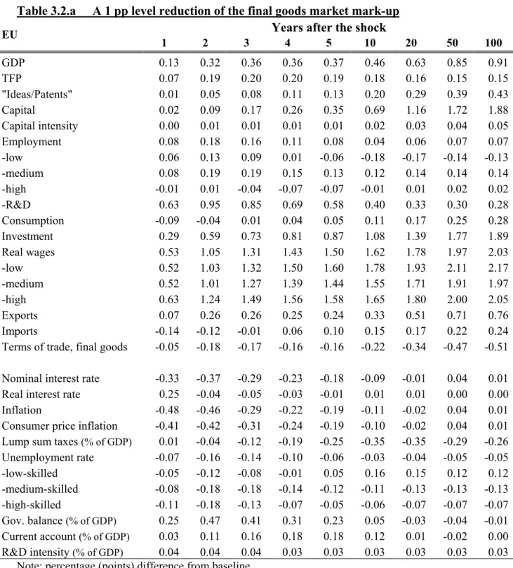
• Reducing product market mark-ups (3.2)

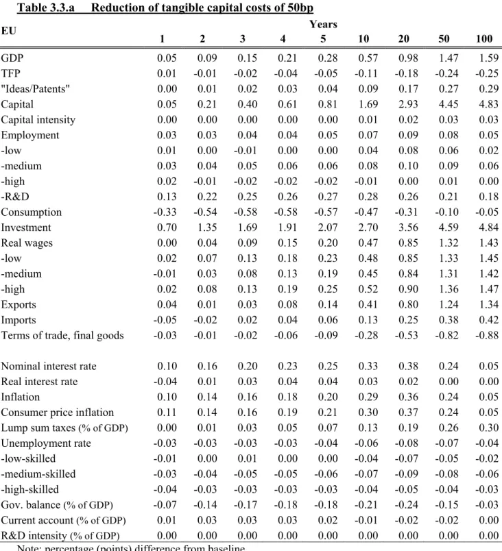
• Reducing capital costs (3.3)

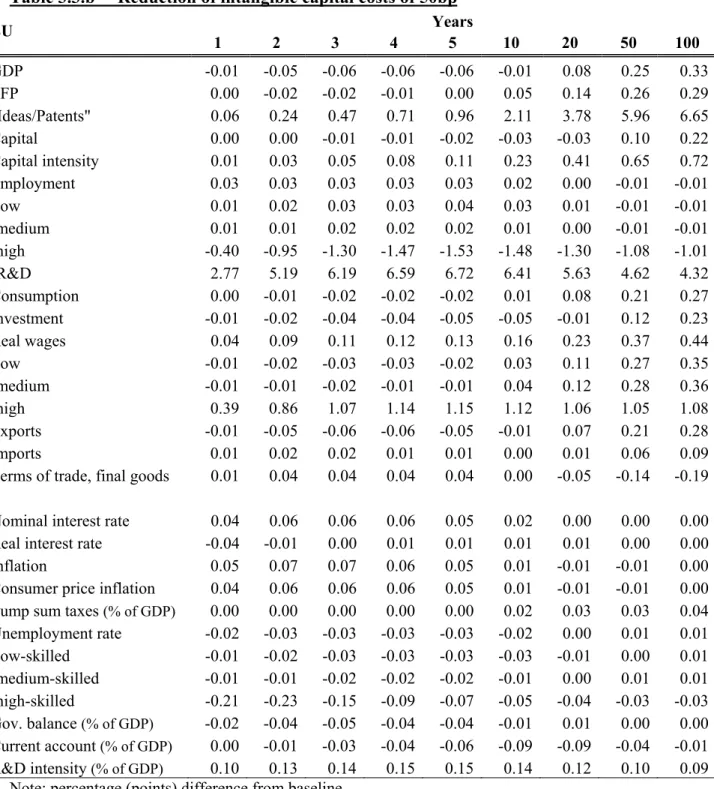
• Reduction in fixed costs (3.4 )

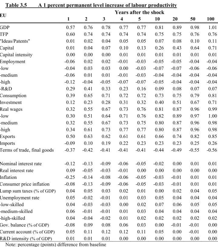
• Exogenous productivity shock (3.5)

• Reducing wage mark-ups (3.6)

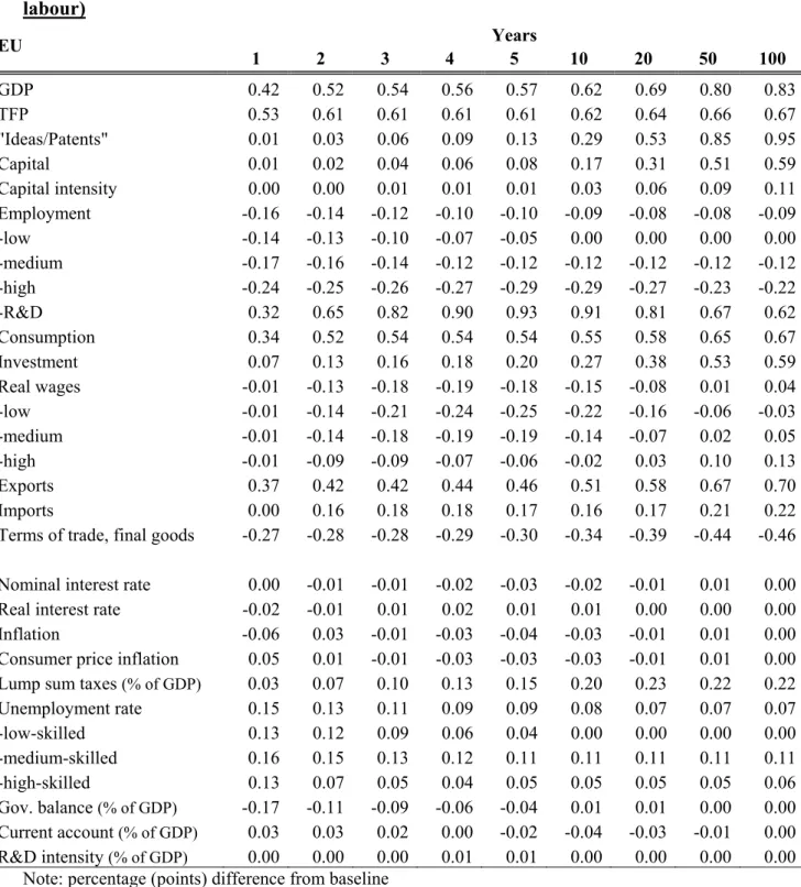
• Tax shifts: from labour to consumption and from low- to high skilled (3.7 and 3.8)

• Reducing benefit generosity (3.9)

• Raising human capital (3.10)

3.1 Raising R&D through tax credits and wage subsidies

The specification of knowledge production in the model presented in this paper is consistent with the often heard argument that market economies underinvest in R&D because individual investors do not fully internalise the external effects from knowledge spillovers. Empirical studies seem to confirm this claim. Estimates of private rates of return13 vary between 8 and 20% (see Coe and Helpman (1995) and Botazzi and Perri (2007)). Estimates of social rates of return based on interfirm technology spillovers vary between 17% (Sveikauskas (1981)) and 100% (Jones and Williams (1998)). The studies by Coe and Helpman as well as Botazzi and Perri also show that there are considerable cross country spillovers. The existence of positive externalities associated with R&D suggests that policies boosting knowledge investment yield social benefits. This section therefore considers two alternative policies. The first scenario is an R&D subsidy in the form of a tax credit (_τA) of 0.1 percent of GDP to the non-liquidity constrained households on their income from intangible capital. Table 3.1.a presents the effects on production, R&D intensity, TFP, R&D labour, total employment and other variables14. Subsidies are financed in a budgetary neutral manner through an increase in lump-sum taxes to households. The simulations show the important characteristic of semi-endogenous growth models: permanent subsidies for R&D-using sectors give a permanent increase in GDP level in the long-run while GDP growth stabilizes. Higher tax-credits allow households to lower the rental rate for intangibles, thus reducing the fixed costs of firms producing intermediates. This in turn raises the demand for blueprints and stimulates R&D and reallocates high skilled workers from production into the research sector. The size of the

h

13 _{The return on R&D is usually defined as the marginal product of the R&D stock. This can be translated into a}

growth effect on TFP by multiplying the social return with the share of R&D in output.

14 _{Note that in t e tables TFP refers to a constructed measure of technological progress defined as}

(

α 1−α

)

/ L K

effect is however rather limited. The results show a 0.08 percent increase in GDP relative to the baseline 20 years after the initial shock and 0.31 percent in the long run. In the long-run the number of employees in the R&D sector increases by around 4 percent and R&D intensity rises by 0.08 percentage points. Notice that it takes time for the output effects to emerge because of short run output losses due to the reallocation of high skilled workers from production to research. Because of supply constraints for high skilled workers part of the fiscal stimulus is offset by wage increases for high skilled workers

Concerning tangible capital stock we have to distinguish between two opposing effects. In the short run, the strong decline of high-skilled labour input in the final goods sector lowers the marginal product of capital which reduces the demand for physical capital. On the other hand higher tax-credits allow non-liquidity constrained households to charge less for intangibles thus reducing the costs of intermediate firms. In the long-run this latter effect unambiguously dominates as technical progress accelerates due to the higher entry rates of intermediate firms. Table 3.1.b shows a scenario in which the subsidy takes the form of a subsidy on the wages of researchers given to the R&D sector. The results show somewhat stronger GDP effects: a 0.1 percent increase in GDP relative to the baseline 20 years after the initial shock and 0.44 percent in the long run. Compared to the R&D subsidy given in the form of tax-credits, this scenario gives more stimulus to the employment of researchers in the long-run: the number of researchers increases by 5.7 percent and R&D intensity rises by 0.12 percentage point.

According to these model simulations wage subsidies in the R&D sector are more efficient than subsidising the use of R&D. It can be shown that the presence of a positive mark-up in the intermediate goods sector lowers the efficiency of the tax credit, while R&D production is assumed to be perfectly competitive. It needs to be further analysed whether this result is robust to imperfections in R&D production. As noted in the literature (see Goolsbee (1998) and Wolff et al. (2008)), there are significant crowding out effects of tax subsidies in the form of higher wages for high skilled workers. This is feature is also present in our simulation experiments. About 25% of the total increase in R&D spending is due to higher wages in these simulations. Goolsbee's estimates for the US range from 30 to 50%.

Table 3.1.a 0.1% of GDP tax-credit R&D subsidy to the non-liquidity constrained households Years EU 1 2 3 4 5 10 20 50 100 GDP -0.01 -0.04 -0.05 -0.06 -0.05 0.00 0.08 0.23 0.31 TFP 0.00 -0.02 -0.02 -0.01 0.00 0.05 0.13 0.24 0.27 "Ideas/Patents" 0.06 0.22 0.44 0.67 0.90 1.97 3.50 5.46 6.04 Capital 0.00 0.00 -0.01 -0.01 -0.02 -0.04 -0.03 0.09 0.21 Capital intensity 0.01 0.02 0.05 0.07 0.10 0.22 0.38 0.59 0.66 Employment 0.03 0.04 0.03 0.03 0.03 0.02 0.01 0.00 0.00 -low 0.02 0.04 0.05 0.06 0.07 0.08 0.07 0.05 0.04 -medium 0.01 0.01 0.01 0.01 0.01 0.00 -0.01 -0.01 -0.02 -high -0.37 -0.89 -1.21 -1.37 -1.43 -1.38 -1.20 -0.98 -0.92 -R&D 2.59 4.85 5.78 6.14 6.26 5.95 5.17 4.20 3.91 Consumption 0.02 0.01 0.00 -0.01 -0.01 0.01 0.07 0.20 0.25 Investment -0.01 -0.03 -0.04 -0.05 -0.05 -0.05 -0.01 0.12 0.21 Real wages 0.04 0.09 0.10 0.11 0.11 0.14 0.21 0.33 0.40 -low -0.02 -0.03 -0.04 -0.05 -0.05 -0.01 0.07 0.22 0.29 -medium -0.01 -0.01 -0.01 -0.01 0.00 0.04 0.12 0.26 0.33 -high 0.37 0.81 1.00 1.07 1.08 1.04 0.98 0.96 0.98 Exports -0.02 -0.06 -0.06 -0.06 -0.05 0.00 0.07 0.20 0.26 Imports 0.02 0.04 0.03 0.02 0.01 -0.01 0.01 0.06 0.08

Terms of trade, final goods 0.01 0.04 0.04 0.04 0.03 0.00 -0.05 -0.13 -0.17 Nominal interest rate 0.03 0.05 0.06 0.05 0.04 0.02 -0.01 0.00 0.00 Real interest rate -0.04 -0.01 0.00 0.01 0.01 0.01 0.01 0.00 0.00 Inflation 0.05 0.07 0.06 0.05 0.04 0.01 -0.01 -0.01 0.00 Consumer price inflation 0.04 0.06 0.06 0.05 0.04 0.01 -0.01 -0.01 0.00 Lump sum taxes (% of GDP) 0.01 0.04 0.06 0.08 0.09 0.14 0.15 0.14 0.14 Unemployment rate -0.02 -0.03 -0.03 -0.03 -0.03 -0.03 -0.02 -0.01 0.00 -low-skilled -0.02 -0.04 -0.05 -0.06 -0.06 -0.07 -0.06 -0.04 -0.04 -medium-skilled -0.01 -0.01 -0.01 -0.01 -0.01 0.00 0.01 0.01 0.01 -high-skilled -0.19 -0.21 -0.14 -0.09 -0.06 -0.04 -0.03 -0.02 -0.02 Gov. balance (% of GDP) -0.11 -0.11 -0.09 -0.08 -0.06 -0.01 0.02 0.00 0.00 Current account (% of GDP) -0.01 -0.02 -0.04 -0.06 -0.08 -0.11 -0.09 -0.03 0.00 R&D intensity (% of GDP) 0.10 0.12 0.13 0.14 0.14 0.13 0.11 0.09 0.08

Table 3.1.b 0.1% of GDP wage subsidy to the R&D sector Years EU 1 2 3 4 5 10 20 50 100 GDP -0.02 -0.06 -0.08 -0.08 -0.08 -0.01 0.11 0.33 0.44 TFP -0.01 -0.03 -0.03 -0.02 -0.01 0.07 0.19 0.34 0.39 "Ideas/Patents" 0.08 0.31 0.62 0.95 1.28 2.82 5.06 7.95 8.83 Capital 0.00 0.00 -0.01 -0.02 -0.02 -0.05 -0.04 0.13 0.29 Capital intensity 0.01 0.03 0.07 0.10 0.14 0.31 0.55 0.86 0.95 Employment 0.04 0.05 0.04 0.04 0.04 0.03 0.01 0.00 -0.01 -low 0.02 0.04 0.05 0.06 0.07 0.06 0.04 0.01 0.01 -medium 0.01 0.02 0.02 0.02 0.02 0.01 0.00 -0.01 -0.02 -high -0.53 -1.27 -1.73 -1.96 -2.05 -1.99 -1.74 -1.43 -1.33 -R&D 3.62 6.85 8.24 8.81 9.01 8.60 7.50 6.11 5.70 Consumption 0.00 -0.01 -0.02 -0.03 -0.02 0.01 0.10 0.28 0.36 Investment -0.01 -0.03 -0.05 -0.06 -0.07 -0.07 -0.02 0.17 0.30 Real wages 0.06 0.12 0.15 0.16 0.17 0.21 0.30 0.48 0.58 -low -0.02 -0.04 -0.04 -0.05 -0.04 0.02 0.13 0.35 0.45 -medium -0.01 -0.02 -0.02 -0.02 -0.01 0.05 0.16 0.37 0.47 -high 0.51 1.14 1.43 1.53 1.55 1.50 1.42 1.39 1.43 Exports -0.02 -0.07 -0.09 -0.08 -0.07 -0.01 0.10 0.28 0.37 Imports 0.02 0.03 0.03 0.02 0.01 0.00 0.01 0.08 0.11 Terms of trade, final goods 0.02 0.05 0.06 0.06 0.05 0.00 -0.07 -0.19 -0.25 Nominal interest rate 0.05 0.08 0.08 0.08 0.07 0.03 -0.01 0.00 0.00 Real interest rate -0.05 -0.01 0.00 0.01 0.01 0.01 0.01 0.00 0.00 Inflation 0.07 0.10 0.09 0.07 0.06 0.01 -0.02 -0.01 0.00 Consumer price inflation 0.06 0.08 0.08 0.08 0.06 0.02 -0.02 -0.01 0.00 Lump sum taxes (% of GDP) 0.01 0.01 0.02 0.04 0.05 0.08 0.09 0.09 0.09 Unemployment rate -0.03 -0.04 -0.04 -0.04 -0.04 -0.03 -0.01 0.00 0.00 -low-skilled -0.02 -0.03 -0.05 -0.05 -0.06 -0.06 -0.03 -0.01 -0.01 -medium-skilled -0.01 -0.02 -0.02 -0.02 -0.02 -0.01 0.00 0.01 0.02 -high-skilled -0.26 -0.30 -0.20 -0.13 -0.09 -0.07 -0.05 -0.04 -0.03 Gov. balance (% of GDP) -0.08 -0.08 -0.08 -0.07 -0.06 -0.01 0.02 0.00 0.00 Current account (% of GDP) 0.00 -0.02 -0.05 -0.07 -0.08 -0.13 -0.12 -0.04 -0.01 R&D intensity (% of GDP) 0.08 0.15 0.18 0.19 0.20 0.19 0.16 0.13 0.12