MPRA
Munich Personal RePEc Archive
Bayesian Analysis of DSGE Models with
Regime Switching
Eo, Yunjong
Washington University in St. Louis
August 2008
Online at
http://mpra.ub.uni-muenchen.de/13910/
Bayesian Analysis of DSGE Models with Regime
Switching
Yunjong Eo
∗Department of Economics
Washington University in St. Louis
Job Market Paper
This Draft: February 11, 2009
†Abstract
I estimate DSGE models with recurring regime changes in monetary policy (inflation target and reaction coefficients), technology (growth rate and volatil-ity), and/or nominal price rigidities. In the models, agents are assumed to know deep parameter values but make probabilistic inference about prevailing and future regimes based on Bayes’ rule. I develop an estimation method that takes these probabilistic inferences into account when relating state variables to observed data. In an application to postwar U.S. data, I find stronger sup-port for regime switching in monetary policy than in technology or nominal rigidities. In addition, a model with regime switching policy that conforms to the long-run Taylor principle given in Davig and Leeper (2007) is preferred to a determinacy-indeterminacy model motivated by Lubik and Schorfheide (2004). These empirical results indicate that, even though a passive policy regime pro-duced more volatility in the economy from the early 1970s to the mid-1980s, the economy can be explained by determinacy over the entire postwar period, implying no role for sunspot shocks in explaining the changes in volatility.
JEL classification: C11, C32, C51, C52, E32, E52
Keywords: New Keynesian DSGE; Markov-switching; Monetary Policy; In-determinacy; Long-run Taylor Principle; Bayesian Analysis;
∗I thank James Bullard, Steven Fazzari, and James Morley for helpful discussions during the initial stages of this research and participants at the Federal Reserve Bank of St. Louis seminar and 2008 MVEA conference for their helpful comments. All errors are mine. Email: [email protected]. Mailing address: Department of Economics, Washington University in St. Louis, Campus Box 1208, St. Louis MO 63130.
1
Introduction
The empirical literature (e.g., Stock and Watson (1996, 2002)) has demonstrated that postwar U.S. macroeconomic data have experienced structural changes with compli-cated patterns such as persistent increases and decreases in means and variances. From a theoretical perspective, agents in the economy should, given these struc-tural changes, have a different understanding about the economy over time and react to the instability. In terms of the U.S. economy, less volatile GDP and inflation since the mid-1980s are the two striking examples of structural changes. Economists have been debating the causes of the “Great Moderation” and two popular explana-tions are improved monetary policy1
and the “Good Luck” hypothesis.2
Meanwhile, even if active monetary policy has stabilized the U.S. economy since the mid-1980s, the source of highly volatile economy before the mid-1980s is not fully understood. Lubik and Schorfheide (2004) have argued that passive monetary policy led to inde-terminacy, implying that sunspot shocks were the cause of higher volatility in the 1970s. By contrast, Davig and Leeper (2007) suggest a theoretical alternative that passive policy generated higher volatility by amplifying “fundamental” shocks under determinacy in the long-run, rather than “sunspot” shocks under indeterminacy. This amplification of fundamental shocks under determinacy occurs if the passive policy is conducted only for short periods of time or the degree of the passive policy is close to the boundary between the active and passive policies. Davig and Leeper refer to the conditions that satisfy determinacy given periods of passive policy as the “long-run Taylor principle.”
I estimate and compare New Keynesian DSGE models with regime changes in order to examine the sources of high volatility of U.S. output and inflation in the 1970s and the so-called “Great Moderation” in the 1980s. I find stronger support for
1
For examples of good monetary policy argument, see Clarida, Gali, and Gertler (2000), Lubik and Schorfheide (2004), and Boivin and Giannoni (2006).
2
For examples of “Good Luck” story, see Stock and Watson (2002), Ahmed, Levin, and Wilson (2004) and Justiniano and Primiceri (2008).
regime switching in monetary policy than in technology or nominal rigidities based on model comparison using marginal likelihoods of models. Also, I find that the long-run Taylor principle-type monetary policy regime switching model is preferred to the determinacy-indeterminacy model. These empirical results mean that, even though a passive policy regime produced more volatility in the economy from the early 1970s to the mid-1980s, the long-run Taylor principle holds over the entire postwar period, implying equilibrium determinacy and no role for sunspot shocks in explaining the changes in volatility.
While motivated by the existing literature, my analysis is distinguished from the conventional New Keynesian model studies in several ways.
First, I endogenously make inference about regime changes and the inferences take into account agents’ probabilistic assessments of regimes. In particular, the response to inflation and output gap in monetary policy, the growth rate and the variance of technology shock, and the nominal rigidity parameter could be dependent on regimes of the economy. I also consider both monetary policy change and stochastic volatility together, but changes are treated as independent, allowing me to isolate the effects of the “Good Luck” and monetary policy on the volatility decline after the early 1980s. Second, the agents in the economy form expectations about key variables in the next period by considering possible regime changes in each period. In particular, transition probabilities are incorporated in model equations directly. This specifica-tion is different from the convenspecifica-tional regime switching analysis such as Hamilton (1989) and Kim and Nelson (1999b) in which the data generating process depends only on the true underlying regimes, rather than probabilistic assessments of regimes, implying that agents know current and past regimes and believe that the current regime will last forever. Meanwhile, the possibility of a transition to other regimes can affect the equilibrium under a given regime and the dynamics in the economy. Davig and Leeper’s (2007) long-run Taylor principle expands the set of determinate rational expectation equilibria. In this paper, I adopt their idea but extend it to
gen-eral regime switching models (e.g., technology, nominal rigidities as well as monetary policy).
Third, building on the literature on Bayesian estimation of DSGE models, I de-velop a method for estimating models with forward-looking regime switching along the lines of the form proposed in Davig and Leeper (2007). They present the long-run Taylor principle theoretically, but they do not examine it in an empirical setting. In order to link observed data to unobservable regime-dependent state variables in multiple regime equations, I integrate the regime-dependent state variables3
in each period over the probability of each regime. The probability of the regime is calculated and updated recursively based on Bayes’ rule every period.
Fourth, I “endogenously” estimate the timing of regime changes in a determinacy-indeterminacy DSGE model that is motivated by Lubik and Schorfheide (2004). This model specification is different from regime switching models discussed above in the sense that the agents in this economy regard the current regime as a permanent regime and do not allow for the possibility of regime changes in the future. How-ever, the parameters for the model are unrestricted, so as to allow for the possibility of indeterminacy. Comparing this determinacy-indeterminacy regime change model with the long-run Taylor principle-type model allows me to determine whether the higher volatilities of economic variables were induced by (i) sunspot shocks when the economy is under indeterminacy or (ii) a passive monetary policy with the long-run Taylor principle holding.
The rest of this paper proceeds as follows. Section 2 introduces forward-looking rational expectations model with regime switching and compare it to conventional regime switching model by using a simple univariate model. Section 3 describes a standard New Keynesian DSGE model without regime switching. Section 4 intro-duces forward-looking rational expectations models with recurring regime changes
3
In Bayesian econometrics, “state variable” often represents a latent variable which governs struc-tural breaks or regime-switchings. However, I use state variables only for unobservable variables in the state-space form in order to avoid confusion.
in the context of DSGE models and shows how to construct a state-space form for these models. Section 5 discusses the endogenous identification of determinacy and indeterminacy in the setting of regime switching analysis. Section 6 explains how to make inferences about model parameters and the probability of regimes in a Bayesian econometrics framework and summarizes empirical results. Section 7 concludes.
2
Illustrative Examples of Forward-Looking Regime
Switching Rational Expectations Models
In this section, I explain how to solve regime switching rational expectations (RSRE) models in which agents in the economy take into account the possibility of regime changes in “deep” parameters. I start with a single equation model with an economic variable. This rational expectations model is a simplification of multivariate dynamic stochastic general equilibrium (DSGE) models but this specification is rich enough to understand the nature of equilibrium. I introduce no regime switching model as a benchmark model at first and consider and compare conventional regime switching and forward-looking regime switching models.
2.1
A constant parameter model
A constant parameter model has an economic variable in a purely forward-looking setting as follows.
xt = aEt[xt+1] +ǫt (1)
ηt = xt−Et−1[xt] (2)
where xt is an endogenous variable, ǫt is a random exogenous shock with i.i.d.
N(0, σ2
ǫ), and ηt is a forecasting error. Before I estimate this model, I need to solve
paper, I use the approach suggested by Sims (2002) and use his notation to describe the rational expectations model. I can rewrite equations (1) and (2) as a matrix form
1 −a 1 0 | {z } Γ0 xt Et[xt+1] | {z } ξt = 0 0 0 1 | {z } Γ1 xt− 1 Et−1[xt] | {z } ξt−1 + 1 0 |{z} Ψ ǫt+ 0 1 |{z} Π ηt. (3)
A solution to equation (3) is a bounded stochastic process ξt. Sims (2002) develops
a solution algorithm and provides conditions on the matrices Γ0, Γ1, Ψ, and Π under which there exists a unique solution (determinacy), multiple solutions (indetermi-nacy), and no solution (explosive process). The nature of equilibrium depends on generalized eigenvalues of matrices (Γ0, Γ1).4
I assume that agents in the economy know the model structure of dynamics5
as well as the model parameters (a,σ2
e). They
can also observe, at time t, history of economic variables {xt, xt−1, xt−2, ...}.
2.2
Purely forward-looking regime switching model
The forward looking regime switching rational expectation (RSRE) model, the focus of this paper, can be distinguished from a conventional regime switching model in the following way. In the forward looking RSRE model, agents take into account the possibility of regime switching in the near future, while in the conventional RSRE model, agents believe that the current regime will last forever. This difference makes the dynamics and equilibrium conditions different given the same model parameters for both models.
To make this model specification simple but still to see the difference between two frameworks, I consider two regimes in the models. However, it is straightforward to extend into more than two regimes and all the properties of dynamics and equilibrium
4
For details, see Sims (2002) and Lubik and Schorfheide (2003, 2004). For the purely forward looking model, if|a|<1, the dynamics is under determinacy, and if|a| ≥1 it is under indeterminacy
and has multiple equilibria.
5
For example, agents understand which variable is included as expectation, current time, and lagged forms in the model.
conditions can be appropriately adjusted. In a conventional regime switching model, the model parameter a in equation (1) can be equal to a1 under the first regime or
a2 under the second regime. Then, given the current regime st = i, equation (1) is
changed to
xt=aiEt[xt+1] +ǫt
and as a matrix form 1 −ai 1 0 | {z } Γ0,st=i xt Et[xt+1] | {z } ξt = 0 0 0 1 | {z } Γ1,st=i xt− 1 Et−1[xt] | {z } ξt−1 + 1 0 |{z} Ψ ǫt+ 0 1 |{z} Π ηt. (4)
Thus, the regime at the previous date t−1 does not directly affect dynamics at the current date t and only ai’s govern the dynamics.
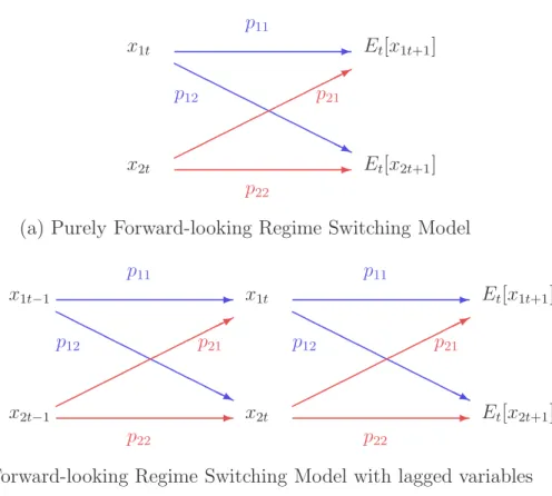
However, in a forward looking RSRE model, if agents know that the current regime can be different from the future regime, this expectation should be reflected when agents make decisions about their behaviors on the current date. For example, even though the current monetary policy is conducted under the passive regime, if agents expect that the passive policy regime will be changed to the active regime in the near future, the effect of the passive policy under the consideration of possibility of switching to the active policy in the near future on the economy could be different from that of a purely passive policy without the possibility of switching to the active regime. This effect of forward looking expectations is described in Figure 1 (a). Agents believe that the probability that the current regime st = i switches to the
regimest+1 =j on the next date ispij. The transition probability matrix for regimes
is P = p 11 p12 p21 p22 .
Thus, given the current regimei, the summation of the probabilities of all the possible regimes on the next date should be equal to one (P2j=1pij = 1 ∀i.).
Figure 1: Structure of Transition Probability: Two regime Model x1t x2t Et[x1t+1] Et[x2t+1] p22 p11 p12 p21 -H H H H H H H H H HHj *
(a) Purely Forward-looking Regime Switching Model
x1t−1 x2t−1 x1t x2t Et[x1t+1] Et[x2t+1] p22 p11 p12 p21 p22 p11 p12 p21 -H H H H H H H H H HHj * -H H H H H H H H H HHj *
I assume that agents also know the transition probabilitypij but do not know the
probability of the current regime. The agents utilize Bayes’ rule to make inference about the probability of the current regime (P[st = i|It]) given currently available
information such as new observation (xit), the probability of each regime at timet−1
(P[st−1 =i|It−1]), the transition probability (pij), and the model structure (likelihood
function). Agents in the economy consider current regime and regime changes in the future when they form the expectations of variables as follows.
Et[xt+1|st=i] =pi1Et[x1t+1] +pi2Et[x2t+1] (5)
where Et[xt+1|st = i] is the expectation of a variable of time t+ 1 at time t given
regime st = i, xit is the value of variable x at time t given regime st =i. I rewrite
this purely forward-looking regime switching model as a matrix form as follows. 1 0 −p11a1 −p12a1 0 1 −p21a2 −p22a2 0 0 1 0 0 0 0 1 | {z } Γ0 x1t x2t Et[x1t+1] Et[x2t+1] | {z } ξt = 0 0 0 0 0 0 0 0 1 0 0 0 0 1 0 0 | {z } Γ1 x1t−1 x2t−1 Et−1[x1t] Et−1[x2t] | {z } ξt−1 + 1 0 0 1 0 0 0 0 | {z } Ψ ǫ 1t ǫ2t | {z } ǫt + 0 0 0 0 1 0 0 1 | {z } Π η 1t η2t | {z } ηt (6)
In this expanded form, the system matrices Γ0, Γ1, and Ψ accommodate directly
transition probabilities (pij, for i, j = 1,2) as well as model parameters. All the
model matrices (Γ0, Γ1, Ψ, Π) are independent of regimes and dates. It depends on the values of pij where i, j = 1,2 as well as αi where i = 1,2 whether the economy
is under determinacy or indeterminacy. For example, even though α2 is less than 1, some appropriate values of α1, p11, and p22 can induce determinacy such as a big value ofα1 ≫1 or a highly persistent p11 close to but less than 1.
Although the regime switching assumption is embedded in the transition equation system, the form of this system is the same as the usual rational expectations form except that the number of equations is the multiplication of the number of regimes and the number of equations in a one regime model. Thus, this rational expectations model can be solved in the same way as the conventional no-regime switching model. This property is different from the conventional regime switching analysis as in equation (4), Hamilton (1989), and Kim and Nelson (1999b). The conventional regime switching models have only regime-dependent parameters and do not include regime change probabilities explicitly in the model dynamics. Thus, the conven-tional approach implicitly solves the raconven-tional expectations model independently for each fixed regime and implies that the agents in the economy believe that the cur-rent regime will last forever and do not think about the possibility of future regime changes.
2.3
Forward-looking Regime-switching model with lagged
vari-able
Similar to the previous case, I adopt the known transition probability assumption for a rational expectations model with lagged variables. The agents also believe that the current regime i at time t comes from the past regime k at time t−1 with the transition probability pki. Notice that, given the regime k at time t − 1 and the
regime i at time t, pki should be the same over the entire periods. If agents’ belief
about the transition probability from the past to the present is time-varying and updated recursively, there is no reason for agents to believe that the transition prob-ability from the present regime to the one period ahead regime is constant as in this paper and literature (e.g. Davig and Leeper (2007) and Farmer, Waggoner, and Zha
(2008)). However, if I allow for recursively updated beliefs about the transition prob-ability, making inferences about this model is computationally infeasible since agents need to update information about transition probability and current regime probabil-ity every period. This simple assumption that the transition probabilprobabil-ity is constant over time enables the expanded state-space form to be a constant parameter model and makes it feasible to determine whether the dynamics of the economy is under determinacy or indeterminacy since the determinacy conditions need to be checked just once rather than every period. In addition, the first order Markov property keeps the number of regimes in history as two rather than 2T when the sample size is T
and the number of regimes at each period is two.
As an extension of equation (1), I introduce a constant parameter model with a lagged variable as follows.
xt =aEt[xt+1] +bxt−1 +ǫt (7)
When considering regime changes in all the parameters, given a regime i the equa-tion (7) changes to
and as a matrix form 1 0 −p11a1 −p12a1 0 1 −p21a2 −p22a2 0 0 1 0 0 0 0 1 | {z } Γ0 x1t x2t Et[x1t+1] Et[x2t+1] | {z } ξt = p11b1 p21b1 0 0 p12b2 p22b2 0 0 1 0 0 0 0 1 0 0 | {z } Γ1 x1t−1 x2t−1 Et−1[x1t] Et−1[x2t] | {z } ξt−1 + 1 0 0 1 0 0 0 0 | {z } Ψ ǫ 1t ǫ2t | {z } ǫt + 0 0 0 0 1 0 0 1 | {z } Π η 1t η2t | {z } ηt . (9)
Then, the algorithm to solve the purely forward-looking RSRE models can be applied to models with lagged variables.
Farmer, Waggoner, and Zha (2008) suggest a method to solve regime-switching models which are linear in variables. I propose a new method to solve more gen-eral regime switching models in the sense that regime switching rational expectations models are non-linear in both variables and parameters. The difference is that eco-nomic state variables in Farmer, Waggoner, and Zha (2008) are not regime-dependent and they turn on and off channels depending on current and previous regimes.
3
A Standard New Keynesian DSGE model
In this paper, I use a standard New Keynesian dynamic stochastic general equilibrium (DSGE) model, which involves three main equations (an IS relationship, a Phillips curve, and a monetary policy rule), two exogenous shock processes (a technology shock and a preference shock), and a log-linear approximation. These equations are
derived in Woodford (2003) and An and Schorfheide (2007) as follows. ˆ xt=Et[ˆxt+1] + ˆgt−Et[ˆgt+1]− 1 τ( ˆRt−Et[ˆπt+1]−Et[ˆzt+1]) (10) ˆ πt =βEt[ˆπt+1] +κ(ˆxt−ˆgt) (11) ˆ Rt=ρRRˆt−1+ (1−ρR)[ψ1πˆt+ψ2xˆt)] +ǫRt (12) ˆ zt =ρgzˆt−1+ǫzt (13) ˆ gt =ρgˆgt−1 +ǫgt (14)
Let ˆxt=ln(xt/x) denote the percentage deviation of a variablext from their
steady-state x where xt = Xt/At is a detrended variable and At is aggregate productivity
at time t. The aggregate productivity At follows a stochastic process with the gross
growth rate γ and the exogenous shock zt:
lnAt =lnγ+lnAt−1+lnzt
wherezt evolves according to univariate AR(1) process in (13).6 Equation (10) is the
intertemporal Euler equation and is derived from the households’ optimization prob-lem whereτ−1
denotes the intertemporal substitution elasticity. Since the model does not include the capital accumulation channel, consumption is proportional to output and perturbed by the exogenous shock gt which follows the AR(1) process in (14).
The shock gt is interpreted broadly as a preference shock as well as a
governmen-tal expenditure shock. The expectational Phillips curve in equation (11) is produced from a continuum of monopolistically competitive firms’ profit maximization problem where κ is a measure of nominal price stickiness due to quadratic adjustment costs and β is the households’ discount factor. The central bank follows a Taylor-type rule by adjusting the nominal interest rate in response to deviations of inflation and
6
Output is directly detrended by estimating the growth rate of the technology and removing the stochastic trend of output in a measurement equation of state-space model form.
output from their steady-state levels. The shockǫRt is the unexpected deviation from
the policy rule. In addition, the central bank is assumed to smooth the policy interest rate.
Let ηπ
t and ηtx denote the expectational errors for the inflation deviation and
output gap at time t given the information time t−1 respectively.
ηπ
t = ˆπt−Et−1[ˆπt]
ηx
t = ˆxt−Et−1[ˆxt]
Moreover, the one period ahead expectation of exogenous shock depends on the cur-rent value of the shock and its persistence:
Et[ˆgt+1] = Et[ρggˆt+ǫgt] = ρggˆt (15)
Et[ˆzt+1] = Et[ρzzˆt+ǫzt] =ρzzˆt. (16)
Substituting (15) and (16) into (10), the IS equation can be expressed in terms of the current period variables. The rational expectations model system includes all the equations and exogenous shock processes which consist of endogenous variables, expectational errors, and exogenous shocks. Thus, the system can be rewritten as a matrix form as follows.
Γ0ξt=Γ1ξt−1+Ψǫt+Πηt
where ξt = [ˆxt,πˆt,Rˆt,Et−1[ˆxt],Et−1[ˆπt],gˆt,zˆt]′, ǫt = [ǫgt, ǫzt, ǫRt]′, and ηt = [ηxt, ηtπ]′.
The matrices Γ0, Γ1, Ψ, and Π contain the appropriate model parameters. Then,
I can easily solve this rational expectations model by using Sims’s gensys code and get a reduced form as follows.
ξt =Gξt−1+Wǫt
capita output: ∆yt, the annualized inflation rate: πt, and the nominal interest rate:
Rt) to unobservable state variables in the transition equation system.
∆yt πt Rt = γQ+ ˆx t−xˆt−1+ ˆzt πA+ 4ˆπ t πA+rA+ 4γQ+ 4 ˆR t = γQ πA πA+rA+ 4γQ | {z } A + 1 0 0 0 0 0 1 −1 0 4 0 0 0 0 0 0 0 0 4 0 0 0 0 0 | {z } B ˆ xt ˆ πt ˆ Rt Et−1[ˆxt] Et−1[ˆπt] ˆ gt ˆ zt ˆ xt−1 | {z } ξt (17)
Note that the lagged variable ˆxt−1, which is not initially included in the vector of
state variables, is augmented in the vector in order to detrend output.
4
New Keynesian DSGE models with Regime
Switch-ing
In the previous section, I briefly outlined the standard log-linearized equations for New Keynesian DSGE models. However, this analysis is distinguished from conven-tional New Keynesian studies. I take account of recurring regime changes in mone-tary policy, technology, and nominal price rigidities. Agents in the economy consider the possibility of the regime changes and know deep parameters but do not know the current regime. Thus, the agents make inference about the current regime in a probabilistic manner by updating their information recursively. The possibility of a
transition to the other regimes can alter the stability conditions and the dynamics in this economy. Davig and Leeper (2007) pointed out this possibility for monetary pol-icy regimes corresponding to active and passive polpol-icy, and introduced a generalized long-run Taylor principle which expands the set of determinate rational expectation equilibrium. In this paper, I adopt their idea but extend it to general regime switching models (e.g., technology, nominal rigidities as well as monetary policy). Throughout this paper, two regimes are taken into account but it is straightforward to develop models with more regimes.
4.1
Regime switching in policy
Davig and Leeper (2007) argue that the passive monetary policy might have induced the higher volatility before 1980s, even with the long-run Taylor principle holding. The idea is that the passive policy for some periods can still generate the determinacy equilibrium if the passive policy is conducted only for short periods of time or the degree of the passive policy is close to the boundary between the active and passive policies. Based on this idea, I endogenously make inference about regime changes from the viewpoint of agents who learn about regimes of the economy. In addition, I allow for regime changes in the smoothing parameter (ρR) and the inflation target
(πA) as well as the reaction coefficients to inflation deviation from the inflation target
(ψ1) and output gap (ψ2). Under a regime i, the monetary policy rule is given by ˆ
Rit = p1iρRiRˆ1t−1+p2iρRiRˆ2t−1+ (1−ρRi)[ψ1iπˆit+ψ2ixˆit] +ǫeit (18)
πA = πiA, i=HorL (19)
and the inflation target is estimated in the measurement equation system as the mean of the annualized inflation rate.7
The mean of inflation is also regime-dependent. I
7
Schorfheide (2005) estimates a monetary policy DSGE model in which the target inflation rate is subject to regime switches. He assumes that the reaction coefficients to inflation and output gap are constant and the entire U.S. postwar economy is under determinacy equilibrium. His analysis
assume that the central bank performs an active monetary policy with low inflation target and a passive monetary policy with high inflation target.
4.2
Regime switching in technology
Stochastic volatility and the so-called “Great Moderation” have featured prominently in the business cycle literature. This Markov-switching structure on volatility can capture these volatility changes in a parsimonious and tractable way and represent “Good Luck” story for the volatility reduction. I explicitly specify this feature by introducing regime changes in technology.
ˆ zit =p1iρzizˆ1t−1 +p2iρzizˆ2t−1+ǫzit, ǫzit ∼ N(0, σ 2 zi) σ 2 z1 < σ 2 z2. (20)
Meanwhile, Hamilton (1989) and Kim and Nelson (1999a) show that a simple Markov-switching regime model can capture business cycle properties by matching estimated probabilities of a recession regime to NBER recession dates. Thus, the growth rate of technology shocks is associated with changes between boom and re-cession in the present regime switching model. Then, given a regime i, the regime switching technology is directly related to the growth rate of output.
∆yit = γiQ+ ˆxit−p1ixˆ1t−1−p2ixˆ2t−1 + ˆzit γiQ = γ Q H or γ Q L (21)
4.3
Regime switching in nominal rigidities
I also consider the possibility of time-varying price stickiness. The idea is that firms have the incentive to reset prices more frequently when the economy faces bigger shocks. Thus, the nominal rigidity parameter κ, which has a negative relationship shows that the inflation target was higher from the mid 1970s to the mid 1980s than other periods.
with price stickiness, may increase in the variance of exogenous productivity shock:
ˆ
πit = βEt[ˆπt+1|st=i]−κi(ˆxt−ˆgt)
= β(pi1Et[ˆπ1t+1] +pi2Et[ˆπ2t+1]) +κi(ˆxit−ˆgit). (22)
The technology shock process for the changes in the volatility is the same as equa-tion (20) but the growth rate of technology shock is constant.
4.4
Construction of state-space form
4.4.1 Transition equations
In forward-looking regime switching rational expectations models, state variables in the state-space form are regime-dependent. Suppose the current regime is st = i
regime. Then, the monetary policy and the expectational Phillips curve equations are modified to equations (18) and (22) respectively. In addition, the IS equation consists of regime-dependent variables as follows.
ˆ xit = Et[ˆxt+1|st=i] + ˆgit−Et[ˆgt+1|st=i]− 1 τi ( ˆRit−Et[ˆπt+1|st=i]−Et[ˆzt+1|st=i]) = pi1Et[ˆx1t+1] +pi2Et[ˆx2t+1] + ˆgit−pi1ρg1ˆgit−pi2ρg2gˆit −1 τi ( ˆRit−pi1Et[ˆπ1t+1]−pi2Et[ˆπ2t+1]−pi1ρz1zˆit−pi2ρz2zˆit) (23)
In equation (23), the expectations of the exogenous shocks are calculated by consid-ering the possibility of regime change from regimei to regime j = 1,2 as
Et[ˆgt+1|st=i] = pi1ρg1gˆit+pi2ρg2gˆit
Et[ˆzt+1|st=i] = pi1ρz1zˆit+pi2ρz2zˆit.
Then, the transition equations are collected in a multivariate equations form. For the case of two regimes, I need to consider two sets of state variables for the transition
equations in the state-space form. Γ0 ˆ x1t ˆ π1t ˆ R1t Et−1[ˆx1t] Et−1[ˆπ1t] ˆ g1t ˆ z1t ˆ x2t ˆ π2t ˆ R2t Et−1[ˆx2t] Et−1[ˆπ2t] ˆ g2t ˆ z2t | {z } ξt = Γ1 ˆ x1t−1 ˆ π1t−1 ˆ R1t−1 Et−2[ˆx1t−1] Et−2[ˆπ1t−1] ˆ g1t−1 ˆ z1t−1 ˆ x2t−1 ˆ π2t−1 ˆ R2t−1 Et−2[ˆx2t−1] Et−2[ˆπ2t−1] ˆ g2t−1 ˆ z2t−1 | {z } ξt−1 +Ψ ǫR1t ǫg1t ǫz1t ǫR2t ǫg2t ǫz2t + Π ηx 1t ηπ 1t ηx 2t ηπ 2t | {z } ǫt
After solving the rational expectations model, the transition equations system can be rewritten as ξ 1t ξ2t =G ξ 1t−1 ξ2t−1 +W ǫ 1t ǫ2t where ξit= h ˆ xit,πˆit,Rˆit,Et−1[ˆxit],Et−1[ˆπit],gˆit,zˆit′ i′ . 4.4.2 Measurement equations
In order to construct a likelihood function, I utilize the Kalman filter given a state-space form of measurement and transition equations. The measurement equations
link observables to unobservable state variables in the transition equation system. However, in forward-looking regime switching models, the measurement equations also contain the probability information of each regime. The measurement equations are constructed by multiplying the probability of each regime up to time t −1 in-formation by the measurement equations of each regime so that regime dependent variables are integrated over the probabilities of each regime.
∆yt πt Rt = 2 X j=1 P[st=j|It−1] γjQ+ (ˆxjt−p1jxˆ1t−1−p2jxˆ2t−1+ ˆzjt) πA j + 4ˆπjt πA j +rA+ 4γ Q j + 4 ˆRjt (24)
In equation (24), the probability of the current regime up to time t−1 information is calculated by multiplying Markov transition probability by probabilities of regimes at timet up to timet−1 information.
P[st =j|It−1] =p1j ×P[st−1 = 1|It−1] +p2j ×P[st−1 = 2|It−1] (25)
The probability of regimest=j at timetis updated recursively based on Bayes’ rule
with data yt = [y 1,· · · , yt]′. P[st=j|It] = P[st=j|yt, It−1] = f(yt, st=j|It−1) f(yt|It−1) = P2f(yt|st=j, It−1)P[st =j|It−1] k=1f(yt|st=k, It−1)P[st=k|It−1] (26)
4.5
Independent regime changes in technology and monetary
policy
I also consider monetary policy changes and stochastic volatility together. The two are treated as independent, allowing us to isolate the effects of “Good Luck” and
monetary policy on volatility reduction after the early 1980s. Thus, this specifica-tion examines whether it was monetary policy or so-called “Good Luck” that played the key role in the “Great Moderation.” For this specification, I introduce two in-dependent regime switching transitions. For example, monetary policy follows the first switching system and stochastic volatility follows the second Markov-switching system. I will take this approach in the next section in order to verify the source of volatility reduction in the latter portion of the sample period. Let P1
and
P2
denote two transition matrices respectively and assume that each regime switching system consists of two regimes. Then, the number of all the possible regimes from two independent structures is four (= 2×2).
P =P1 ⊗P2 and st= 1 if (s1t = 1, s2t= 1) st= 2 if (s1t = 1, s2t= 2) st= 3 if (s1t = 2, s2t= 1) st= 4 if (s1t = 2, s2t= 2) (27)
where ⊗ denotes the Kronecker product. Then, as in (25)
P[sit =j|It−1] =p
i
1j×P[sit−1 = 1|It−1] +p
i
Updating the probability of the current regime by observing data at time t is given by P[sit =j|It] = P[sit =j|yt, It−1] = f(yt, sit =j|It−1) f(yt|It−1) = P2 f(yt|sit =j, It−1)P[sit =j|It−1] l=1 P2 k=1f(yt|sit=k, s−it=l, It−1)P[sit =k, s−it=l|It−1] = P2 l=1f(yt|sit =j, s−it=l, It−1)P[sit=j, s−it =l|It−1] P4 k=1f(yt|st =k, It−1)P[st=k|It−1] .
where the subscript −i ins−it indicates any regime −i6=i
5
Endogenous Identification of Determinacy and
Indeterminacy Equilibria
Following the idea of Clarida, Gali, and Gertler (2000), Lubik and Schorfheide (2004) show, using a DSGE model, that a change in monetary policy can explain higher volatility in pre-Volcker years. They argue that the passive monetary policy led to indeterminacy, implying that sunspot shocks played a role in generating the higher volatility. They split postwar U.S. data into two subsamples “exogenously” based on the appointment of Paul Volcker as Chairman of the Board of Governors of the Fed-eral Reserve system and excluding Volcker disinflation period (1979:Q4 to 1982:Q3). I estimate the determinacy-indeterminacy regime switching DSGE model and “endoge-nously” identify two regimes. The agents in this economy regard the current regime as a permanent regime and do not allow for the possibility of regime changes in the future. Thus, technically I solve the rational expectations model for each regime separately and estimate regime changes by adopting a conventional regime-switching estimation technique. This model specification allows for determining whether the
higher volatilities of economic variables are induced by (i) a passive monetary policy with the long-run Taylor principle holding or (ii) sunspot shocks when the economy is under indeterminacy. In this paper, Hamilton’s filter and Kim’s filter enable me to estimate this model. For more details about Hamilton’s filter see Hamilton (1989) and Hamilton (1994), and about Kim’s filter see Kim (1994) and Kim and Nelson (1999b).
6
Bayesian Estimation
6.1
Methodology
I develop a method to estimate forward-looking regime switching models. Davig and Leeper (2007) present the long-run Taylor principle theoretically, but they do not examine it in an empirical setting. In addition, they take into account only the transition equations. However, I append the model with measurement equations in order to evaluate a likelihood function through Kalman filtering for the state-space form as in (24). Econometricians observe one data set but transition equations and unobservable regime dependent variables such as xit in (5) are based on multiple
regimes. Thus, I integrate state variables over the probabilities of each regime in order to match them to the observables. The probability of the regime is calculated and updated recursively based on Bayes’ rule every period as in (25) and (26). While agents in the economy know deep parameter values, they do not know the current regime and so they are learning about it. I, as an econometrician, estimate model parameters and probabilities of regimes each period.
I estimate and compare various regime switching models with a likelihood-based approach. by adopting the Metropolis-Hastings (MH) algorithm with randomized multiple blocks. Chib and Greenberg (1995) suggest the use of fat-tailed proposal to ensure that proposed values visit the tails of the posterior distributions and I use three blocks of parameters and Student-t distributed errors with the degrees of
freedom of 15. In particular, Chib and Ramamurthy (2008) develop an approach that randomly generates blocks and finds a proposal density for each block by adapting the location and curvature and holding other blocks fixed at every iteration. Although the random-walk MH proposal with a single block, most of likelihood-based DSGE estimations have used, is faster and convenient to calculate marginal likelihoods, the recent literature advocates the use of the randomized multiple blocks in DSGE models due to following reasons. An and Schorfheide (2007) show that the single block random-walk proposal often gets stuck at a local posterior mode. In such a case, the performance and reliability of the MH algorithm are sensitive to the starting point, making it important to find the global posterior mode accurately. In addition, Sims, Waggoner, and Zha (2008) point out that it takes multiple weeks of CPU time to find the posterior mode especially in large Markov-switching models and propose the use of a blockwise optimization method. Chib and Ramamurthy’s (2008) idea is similar to the blockwise optimization but it is more reliable in the sense that this algorithm reoptimizes over iterations and the simulation does not hinge on the starting point which is possibly a local mode. In particular, having adopted multiple blocks, it is not known which parameters should be in the same block. In New Keynesian DSGE models, all the parameters are highly-nonlinearly related by model equations and their equilibrium conditions. Thus, the randomized block scheme is an alternative approach.
This analysis is based on postwar U.S. quarterly data from 1960:Q1 to 2007:Q4. The estimation of model parameters and probability of regimes can be affected by initial values of state variables and regime probabilities. Thus, the initial values are determined from pre-sample period from 1954:Q1 to 1959:Q4. I restrict parameter space to induce determinacy equilibrium in the forward-looking regime switching models, but the determinacy-indeterminacy regime switching model obviously allows for both determinacy and indeterminacy regimes.
6.2
Model priors
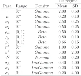
The models are characterized in Table 1 and priors are listed in Table 2. In the Table 1: DSGE Models with Regime-Switching
Model Regime-Switching parameters
M0: No regime switching None
M1: Growth rate of technology γQ
M2: Monetary policy ψ1,ψ2,πA, ρR M3: Variance of tech. shock σz
M4: Price stickiness and variance of tech. κ, σz
M5: Monetary policy(1st); Variance of tech.(2nd) 1st: ψ1,ψ2,πA, ρ
R; 2nd: σz
regime switching models, I regard the first regime as ordinary (e.g., active monetary policy, boom, or less volatile economy) and the second regime as unusual (e.g., passive monetary policy, recession, or highly volatile economy). Model M0 is a benchmark model without regime switching. Priors for the “no regime switching” model and the first regime in the various regime switching models are similar to An and Schorfheide (2007) except for some key parameters related to regime switching. Among regime switching models, model M1 allows for regime switching for growth rate of produc-tivity. Hamilton (1989) applied his Markov-switching model of univariate autore-gressive regression to U.S. real GNP growth and found that the MLE estimate of the growth rate under the recession regime is -0.36. Thus, the prior for the growth rate under the recession regime is a Normal distribution with mean -0.2 and stan-dard deviation 0.2 while the prior mean of growth rate under the usual regime is 0.6 with standard deviation 0.2. The regime change in monetary policy is exam-ined in model M2. I choose priors for reaction coefficients to inflation and output gap consistent with those of the previous literature such as Clarida, Gali, and Gertler (2000) and Lubik and Schorfheide (2004). The prior of the inflation coefficient is a Gamma distribution with mean 2.50 and standard deviation 0.25 under the active policy regime, while 0.50 and 0.25 respectively under the passive policy regime. I also allow for change in smoothing policy parameter ρR. Notice that the prior for
an autoregressive coefficient ρR is the same across regimes with a Beta distribution
with mean 0.5 and standard deviation 0.2 so that it is reasonably diffuse. ModelM3 represents the so-called “Good Luck” story or stochastic volatility. In this model, the technology shock is the main source of fluctuations in the economy so that only the variance of technology shock is allowed to change. I estimate standard deviations for variances of shocks rather than variances directly and the standard deviation has an Inverse Gamma distribution. Model M4 incorporates regime changes in nominal rigidities in response to the size of exogenous productivity shock. Since the price rigidity parameter κincreases in the volatility of technology shock, the prior mean is 0.2 under the ordinary regime and 0.4 under the high volatile regime. In model M5, there are two independent regime switching systems in order to identify the source of “Great Moderation,” as explained in the previous section. One regime switching system is related to the stochastic technology shock and the other is related to the monetary policy. I complete this section by explaining priors for the transition prob-abilities. All the transition probabilities pii where i = 1,2 have a Beta distribution
with mean 0.9 and standard deviation 0.09. This prior is diffuse enough not to affect making inferences about probabilities of regimes.
6.3
Empirical results
I compare various models with marginal likelihood calculations and report the nature of regime switching in postwar U.S. economy. The marginal density calculations are based on Chib and Ramamurthy (2008). Given model Ms, the marginal density
m(y|Ms) can be written as
m(y|Ms) = π(θ, P)f(y|θ, P)
π(θ, P|y)
Then, for anyθ, basic marginal likelihood identity holds and the logarithm of marginal likelihood of modelMscan be estimated atθ∗, which is usually the mode of posterior
Table 2: Priors for no regime-switching model 1st regime Para Range Density Mean SD
τ R+ Gamma 2.00 0.50 κ R+ Gamma 0.20 0.10 ψ1 R+ Gamma 2.50 0.25 ψ2 R+ Gamma 0.50 0.25 ρR [0,1) Beta 0.50 0.20 ρg [0,1) Beta 0.80 0.10 ρz [0,1) Beta 0.66 0.15 rA R+ Gamma 1.00 0.50 πA R+ Gamma 5.00 2.00 γQ R Normal 0.60 0.20 σR R+ InvGamma 0.40 4.00 σg R+ InvGamma 0.20 4.00 σz R+ InvGamma 0.20 4.00
Table 3: Priors for regime-switching model 1st regime 2nd regime Para Range Density Mean SD Mean SD
κ R+ Gamma 0.20 0.10 0.40 0.10 ψ1 R+ Gamma 2.50 0.25 0.50 0.25 ψ2 R+ Gamma 0.50 0.25 0.50 0.25 ρR [0,1) Beta 0.50 0.20 0.50 0.20 πA R+ Gamma 5.00 2.00 7.00 2.00 γQ R Normal 0.60 0.20 - 0.20 0.20 σz R+ InvGamma 0.20 4.00 1.00 4.00 pii [0,1) Beta 0.90 0.09 0.90 0.09
Notes: Priors for parameters which is not subject to regime-switching are adopted from priors for parameters in no-regime switching model.
density,
lnmˆ(y|Ms) = lnf(y|θ∗,Ms) +lnπ(θ∗|Ms)−lnπˆ(θ∗|y,Ms).
The estimates of marginal likelihoods are reported in Table 4. Based on the marginal likelihood calculations, the monetary policy regime switching model is selected. Thus, I focus most of my discussion on the “no regime switching” model M0 and the monetary policy model M2.
Table 4: Model Comparison and Marginal Likelihood
Model Log-Marginal Likelihood
M0: No regime switching -923.02
M1: Growth rate of technology -896.16
M2: Monetary policy -830.82
M3: Variance of tech. shock -870.64
M4: Price stickiness and variance of tech. -855.71
M5: Monetary policy(1st); Variance of tech.(2nd) -835.23
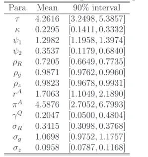
Table 5: Posteriors for no regime-switching model Para Mean 90% interval
τ 4.2616 [3.2498,5.3857] κ 0.2295 [0.1411,0.3332] ψ1 1.2982 [1.1958,1.3974] ψ2 0.3537 [0.1179,0.6840] ρR 0.7205 [0.6649,0.7735] ρg 0.9871 [0.9762,0.9960] ρz 0.9823 [0.9678,0.9931] rA 1.7063 [1.1049,2.1890] πA 4.5876 [2.7052,6.7993] γQ 0.2047 [0.0500,0.4804] σR 0.3415 [0.3098,0.3768] σg 1.0698 [0.9752,1.1757] σz 0.0958 [0.0787,0.1168]
I begin by looking at results from no regime switching model (M0). The posterior distributions are summarized in Table 5. In this model, the inflation reaction
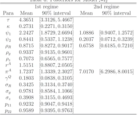
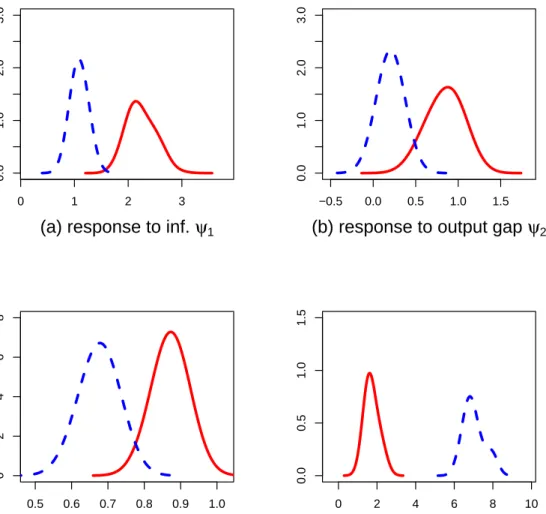
coeffi-cient in monetary policy from the posterior distribution is greater than one, at least according to the 90% credible set. In the monetary policy regime switching model (M2), under the active policy regime, the central bank increases the nominal interest rate by 2.25 percent (posterior mean) in response to 1 percent inflation deviation from the target while it adjusts 1.09 percent under the passive regime. These coeffi-cient estimations are close to 2.19 and 0.89 respectively that Lubik and Schorfheide (2004) attained in subsample analysis. Although the posterior mean of the coeffi-cient under the passive regime from Lubik and Schorfheide’s (2004) estimation is below one and my estimate of the posterior mean is greater than one, the 90% credible set of the coefficient under the passive regime includes a lot of mass be-low one. This fact is illustrated well in Figure 2 and reported in Table 6. Note that in Lubik and Schorfheide (2004) the passive regime was driven by indeterminacy in the pre-Volcker years. However, this regime switching analysis shows that even the passive monetary policy induced a determinacy equilibrium in the long run due to the possibility of the switching to active policy, although the passive policy could be a source of high volatility.8
In this scenario, the postwar U.S. economy experienced two regime switching points around early 1970s from active to passive policy and around mid-1980s from passive to active policy as shown in Figure 3. In addition, the target inflation was high with 7.02 comparing to 1.72 under the active regime. It also reflects the “Great Inflation” of the 1970s. Although the transition matrix for the regime switching is not restricted to generate persistent regimes a priori, agents’ belief about regimes clearly looks like two structural breaks. In addition, the second regime switching point is consistent with the estimate of a structural break in the form of a volatility reduction in Kim and Nelson (1999a) and McConnell and Perez-Quiros (2000). As for other parameters that are subject to regime switching, the reaction to the output gap is more aggressive in the active policy regime (0.84 vs 0.20) and the
8
Boivin and Giannoni (2006) performed VAR analyses and counterfactual experiments and showed that the strong response to inflation expectations stabilizes the economy in the post-1980 period.
Figure 2: Posterior Distributions from Monetary Policy Regime Switching Model (M2) 0 1 2 3 0.0 1.0 2.0 3.0
(a) response to inf. ψ1
−0.5 0.0 0.5 1.0 1.5
0.0
1.0
2.0
3.0
(b) response to output gap ψ2
0.5 0.6 0.7 0.8 0.9 1.0 0 2 4 6 8
(c) interest rate smoothing ρR
0 2 4 6 8 10 0.0 0.5 1.0 1.5 (d) inflation target π*
Notes: The solid line (dashed line) represents posteriors from active policy (passive policy).
Figure 3: Probability of Passive Monetary Policy Regime (M2) (P[st = passive policy|It])
0.0
0.2
0.4
0.6
0.8
1.0
60
65
70
75
80
85
90
95
00
05
Table 6: Posteriors for Model M2 1st regime 2nd regime Para Mean 90% interval Mean 90% interval
τ 4.3651 [3.3126,5.4667] κ 0.2731 [0.2271,0.3150] ψ1 2.2427 [1.8729,2.6694] 1.0886 [0.9407,1.2572] ψ2 0.8441 [0.5337,1.1238] 0.2037 [0.0712,0.3239] ρR 0.8715 [0.8272,0.9017] 0.6758 [0.6185,0.7210] ρg 0.9337 [0.9135,0.9601] ρz 0.7073 [0.6565,0.7577] rA 1.5151 [0.8807,2.0505] πA 1.7237 [1.3339,2.3027] 7.0170 [6.2986,8.0015] γQ 0.1803 [0.0838,0.3105] σR 0.3425 [0.3134,0.3740] σg 0.9781 [0.8584,1.1066] σz 0.3908 [0.3155,0.4693] p11 0.9232 [0.9047,0.9418] p22 0.9589 [0.9395,0.9763]
nominal interest rate adjustment involves more smoothing in the active policy regime (0.83 vs 0.68). This finding is consistent with the argument of Bullard and Mitra (2007) that the monetary policy inertia helps induce determinacy equilibrium given the degree of response to inflation discrepancy.
I also estimate the determinacy-indeterminacy model. In terms of timing, the probability of the indeterminacy regime in postwar U.S economy has a similar pat-tern to the probability of the passive regime from a forward-looking monetary policy regime-switching model. The marginal likelihood calculation shows that the marginal likelihood of the determinacy-indeterminacy model is -887.23 while the forward-looking rational expectations model fits postwar U.S. data better with a marginal likelihood of -830.82. From this analysis, I can conclude that the long-run Taylor principle holds in the entire postwar U.S. economy.
7
Conclusion
I estimate DSGE models with recurring regime changes in monetary policy (inflation target and reaction coefficients), technology (growth rate and volatility), and/or nom-inal price rigidities. In the models, agents are assumed to know deep parameter values but make probabilistic inference about prevailing regimes based on Bayes’ rule and form the one period ahead expectations by taking account of possibilities of regime changes. Building on a literature on Bayesian estimation of DSGE models, I develop a method for estimating models with forward-looking regime switching along the lines of the form proposed in Davig and Leeper (2007). In an application to postwar U.S. data, I find stronger support for regime switching in monetary policy than in tech-nology or nominal rigidities. Under the active policy regime, the policy reaction to deviations from the targets of inflation and output was more aggressive and the nomi-nal interest rate adjustment is smoother. I also estimate a determinacy-indeterminacy DSGE model and compare this specification to the Davig and Leeper-type monetary policy DSGE model. A marginal likelihood based model selection procedure prefers the monetary policy regime switching model. This empirical finding implies that even though a passive policy regime produced more volatility in the economy from the early 1970s to the mid-1980s, the long-run Taylor principle appears to hold in the entire postwar period, implying equilibrium determinacy and there is no role for sunspot shocks in explaining the changes in volatility.
References
Ahmed, S., A. Levin, and B. A. Wilson (2004): “Recent U.S. Macroeconomic Stability: Good Policies, Good Practices, or Good Luck?,” The Review of Eco-nomics and Statistics, 86(3), 824–832.
An, S., andF. Schorfheide(2007): “Bayesian Analysis of DSGE Models,” Econo-metric Reviews, 26(2-4), 113–172.
Boivin, J., and M. P. Giannoni (2006): “Has Monetary Policy Become More Effective?,”The Review of Economics and Statistics, 88(3), 445–462.
Bullard, J., and K. Mitra (2007): “Determinacy, Learnability, and Monetary Policy Inertia,”Journal of Money, Credit and Banking, 39(5), 1177–1212.
Chib, S., and E. Greenberg (1995): “Understanding the Metropolis-Hastings Algorithm,” The American Statistician, 49(4), 327–335.
Chib, S., and S. Ramamurthy(2008): “MCMC Methods for Bayesian Estimation of DSGE Models,” Working Paper.
Clarida, R., J. Gali, and M. Gertler (2000): “Monetary Policy Rules And Macroeconomic Stability: Evidence And Some Theory,” The Quarterly Journal of Economics, 115(1), 147–180.
Davig, T., and E. M. Leeper(2007): “Generalizing the Taylor Principle,” Amer-ican Economic Review, 97(3), 607–635.
Farmer, R. E., D. F. Waggoner, and T. Zha (2008): “Minimal state variable solutions to Markov-switching rational expectations models,” Working Paper 2008-23, Federal Reserve Bank of Atlanta.
Hamilton, J. D. (1989): “A New Approach to the Economic Analysis of Nonsta-tionary Time Series and the Business Cycle,” Econometrica, 57(2), 357–84.
(1994): Time Series Analysis. Princeton University Press.
Justiniano, A., and G. E. Primiceri (2008): “The Time-Varying Volatility of Macroeconomic Fluctuations,”The American Economic Review, 98(3), 604–641.
Kim, C.-J. (1994): “Dynamic linear models with Markov-switching,” Journal of Econometrics, 60(1-2), 1–22.
Kim, C.-J., andC. R. Nelson(1999a): “Has The U.S. Economy Become More Sta-ble? A Bayesian Approach Based On A Markov-Switching Model Of The Business Cycle,” The Review of Economics and Statistics, 81(4), 608–616.
(1999b): State-Space Models with Regime Switching: Classical and Gibbs-Sampling Approaches with Applications. The MIT Press.
Lubik, T. A., and F. Schorfheide (2003): “Computing Sunspot Equilibria in Linear Rational Expectations Models,” Journal of Economic Dynamics and Con-trol, 28(2), 273–285.
(2004): “Testing for Indeterminacy: An Application to U.S. Monetary Pol-icy,” American Economic Review, 94(1), 190–217.
McConnell, M. M., and G. Perez-Quiros (2000): “Output Fluctuations in the United States: What Has Changed since the Early 1980’s?,” American Economic Review, 90(5), 1464–1476.
Schorfheide, F. (2005): “Learning and Monetary Policy Shifts,” Review of Eco-nomic Dynamics, 8(2), 392–419.
Sims, C. A.(2002): “Solving Linear Rational Expectations Models,”Computational Economics, 20(1-2), 1–20.
Sims, C. A., D. F. Waggoner, and T. Zha (2008): “Methods for inference in large multiple-equation Markov-switching models,” .
Stock, J. H., and M. W. Watson (1996): “Evidence on Structural Instability in Macroeconomic Time Series Relations,”Journal of Business & Economic Statistics, 14(1), 11–30.
(2002): “Has the Business Cycle Changed, and Why?,” NBER Macroeco-nomics Annual, 17, 159–218.
Woodford, M. (2003): Interest and Prices: Foundations of a Theory of Monetary Policy. Princeton University Press.
Appendix
Figure 4: Probability of Low Growth Rate Regime (M1)
0.0 0.2 0.4 0.6 0.8 1.0 65 70 75 80 85 90 95 00 05
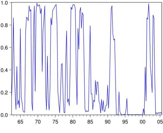
Figure 5: Probability of Large Exogenous Shock Regime (M3)
0.0
0.2
0.4
0.6
0.8
1.0
60
65
70
75
80
85
90
95
00
05
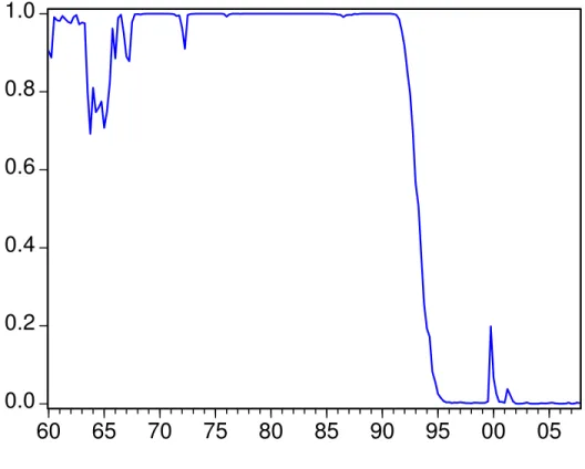
Figure 6: Probability of Large Exogenous Shock with Less Sticky Price Regime (M4)
0.0
0.2
0.4
0.6
0.8
1.0
60
65
70
75
80
85
90
95
00
05
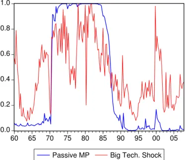
Figure 7: Probabilities of Passive Monetary Policy Regime and Large Exogenous Shock Regime (M5) 0.0 0.2 0.4 0.6 0.8 1.0 60 65 70 75 80 85 90 95 00 05
Passive MP Big Tech. Shock
(a)P[st= Passive Monetary Policy|It] : Blue line
Table 7: Posteriors for Model M1 1st regime 2nd regime Para Mean 90% interval Mean 90% interval
τ 4.8187 [3.5287,6.4544] κ 0.2834 [0.1788,0.4246] ψ1 1.4088 [1.1262,1.8839] ψ2 1.3359 [0.5957,2.3099] ρR 0.7408 [0.6612,0.8309] ρg 0.9760 [0.9550,0.9889] ρz 0.7115 [0.5538,0.8273] rA 1.1799 [0.3895,2.0672] πA 3.9586 [1.8065,6.3989] γQ 0.2485 [0.0602,0.4706] -0.1554 [−0.5596,0.1945] σR 0.3355 [0.2888,0.3926] σg 0.8383 [0.6377,1.2158] σz 0.4162 [0.2623,0.6075] p11 0.9771 [0.9007,0.9988] p22 0.9152 [0.8774,0.9562]
Table 8: Posteriors for Model M3 1st regime 2nd regime Para Mean 90% interval Mean 90% interval
τ 4.3690 [3.2896,5.5264] κ 0.3329 [0.2377,0.4829] ψ1 1.3292 [1.0285,1.8445] ψ2 0.8540 [0.2059,1.6429] ρR 0.7685 [0.6908,0.8288] ρg 0.9629 [0.9387,0.9837] ρz 0.5528 [0.3667,0.6963] rA 1.0613 [0.3524,1.7039] πA 2.0511 [1.5754,2.4774] γQ 0.1697 [0.0632,0.2734] σR 0.3537 [0.3012,0.4125] σg 0.7650 [0.6285,0.9569] σz 0.1818 [0.1136,0.2825] 0.7092 [0.5221,0.8820] p11 0.9897 [0.9777,0.9982] p22 0.9490 [0.9340,0.9667]
Table 9: Posteriors for Model M4 1st regime 2nd regime Para Mean 90% interval Mean 90% interval
τ 4.2980 [3.3131,5.3196] κ 0.2128 [0.1411,0.3039] 0.2950 [0.2160,0.4449] ψ1 1.2886 [1.0506,1.5713] ψ2 0.7562 [0.3721,1.2294] ρR 0.7491 [0.6825,0.8017] ρg 0.9749 [0.9536,0.9889] ρz 0.5266 [0.3486,0.6847] rA 1.1281 [0.4433,1.6643] πA 2.0316 [1.7372,2.4613] γQ 0.1490 [0.0438,0.2713] σR 0.3631 [0.3134,0.4184] σg 0.7721 [0.5737,0.9198] σz 0.2133 [0.1151,0.3636] 0.7085 [0.5218,0.9092] p11 0.9879 [0.9754,0.9979] p22 0.9546 [0.9426,0.9659]
Table 10: Posteriors for Model M5 1st regime 2nd regime Para Mean 90% interval Mean 90% interval
τ 4.8929 [3.3554,6.7933] κ 0.2632 [0.1781,0.3665] ψ1 2.6329 [1.9647,3.2367] 0.8905 [0.8012,0.9791] ψ2 1.2318 [0.4302,2.1938] 1.9685 [0.9157,3.0793] ρR 0.9084 [0.8591,0.9499] 0.5006 [0.3406,0.7062] ρg 0.9700 [0.9367,0.9897] ρz 0.5297 [0.2847,0.7639] rA 1.7654 [0.8646,2.6793] πA 2.3075 [1.2003,3.1614] 6.2472 [3.4939,9.7099] γQ 0.2354 [0.0315,0.4456] σR 0.2495 [0.1408,0.3903] σg 1.1079 [0.8945,1.3847] σz 0.2451 [0.0185,0.5884] 1.2624 [0.6318,1.9460] p11 0.8722 [0.8301,0.9494] 0.6281 [0.4646,0.7240] p22 0.9952 [0.9872,0.9988] 0.8258 [0.7275,0.8967]
![Figure 3: Probability of Passive Monetary Policy Regime (M 2 ) (P[s t = passive policy|I t ]) 0.00.20.40.60.81.0 60 65 70 75 80 85 90 95 00 05](https://thumb-us.123doks.com/thumbv2/123dok_us/1227450.2665829/32.918.186.710.424.843/figure-probability-passive-monetary-policy-regime-passive-policy.webp)