Range-Point Migration-Based Image Expansion Method Exploiting Fully Polarimetric Data for UWB Short-Range Radar

(1)

Range-Point Migration-Based Image Expansion

Method Exploiting Fully Polarimetric Data for

UWB Short-Range Radar

著者（英）

Ayumi Yamaryo, Tatsuo Takatori, Shouhei

Kidera, Tetsuo Kirimoto

journal or

publication title

IEEE Transactions on Geoscience and Remote

Sensing

volume

56 number

4 page range

2170-2182

year

2018-04

URL

http://id.nii.ac.jp/1438/00008863/

doi: 10.1109/TGRS.2017.2776274

(2)

Range Points Migration Based Image Expansion Method

Exploiting Fully Polarimetric Data

for UWB Short Range Radar

Ayumi Yamaryo,

Non-member,

Tatsuo Takatori,

Non-member,

Shouhei Kidera,

Member, IEEE,

and Tetsuo

Kirimoto,

Senior Member, IEEE,

Abstract—Ultra wideband (UWB) radar with high range resolution is a promising technology for use in short-range 3-dimensional (3-D) imaging applications, in which optical cameras are not applicable. One of the most efficient 3-D imaging methods is the range point migration (RPM) method, which has a definitive advantage for synthetic aperture radar (SAR) approach in terms of computational burden, high accuracy and high spatial resolution. However, if an insufficient aperture size or angle is provided, these kind of method cannot reconstruct the whole target structure, due to absence of reflection signals from large part of target surface. To expand the 3-D image obtained by RPM, this paper proposes an image expansion method by incorporating the RPM feature and fully polarimetric data based machine learning approach. Following ellipsoid-based scattering analysis and learning with a neural network, this method expresses the target image as an aggregation of parts of ellipsoids, which significantly expands the original image by the RPM method without sacrificing reconstruction accuracy. The results of numerical simulation based on 3-D finite difference time domain (FDTD) analysis verify the effectiveness of our proposed method, in terms of image expansion criteria.

Index Terms—UWB radars, Short range sensing, 3-D sensors, Fully polarimetric analysis, Range Points Migration(RPM), Im-age expansion

I. INTRODUCTION

U

Ltra wideband(UWB) pulse radar is expected to be adopted in innovative short-range sensing techniques, such as robotic sensors in disaster rescue situations or private watch sensors for independently living elderly or disabled persons. To provide accurate high resolution 3-D images, researchers have investigated various radar imaging methods based on data synthesis, such as synthetic aperture radar(SAR) [1], time-reversal algorithms [2], [3], and range migration methods [4], [5], [6]. However, all of these methods incur impractically large computational costs, particularly in 3-D imaging problems, and their reconstruction accuracies are insufficient to capture the detailed structures of target shapes. As a different approach, the method [7] has been developed, which is based on reversible transforms, namely, boundary scattering transform (BST). While this method achieves a fast 3-D imaging in specifying boundary extraction, it suffers from serious accuracy degradation in noisy or interfered cases assuming multiple or complex-shaped targets due to being based on the difference operation of observed ranges. In A. Yamaryo is with Communication Systems Center Mitsubishi Electric Corp., Japan. T. Takatori, S. Kidera and T. Kirimoto are with the Grad-uate School of Informatics and Engineering, The University of Electro-Communications, Tokyo, Japan. E-mail: [email protected]

contrast, the range point migration(RPM) method extracts the 3-D target boundary even in noisy or richly interfered case [8], [9], [10]. The RPM method assesses the distribution function of the direction of arrival (DOA) for each observed range point (denoted as a set of antenna location and range), and does not require any paring procedure of discrete range points as pre-processing. It also accomplishes highly accurate 3-D imaging for general target shape in far less computation costs than that required by conventional signal synthesis approaches such as 3-D beamforming or SAR based reconstruction scheme. The effectiveness of RPM has been widely reported in short-range radar and acoustic imaging studies [11], [12], [13]. However, the image reproduction area obtained by RPM and other conventional methods is, usually severely limited by an available aperture angle, determined by the aperture size and distance to target, which is itself restricted by obstacles such as rubble in disaster zones and indoor sensing problems. For these reasons, the reconstructed area frequently becomes too narrow to identify the target structure, and this is an essential problem in any kind of imaging methods as far as they use only direct reflection signal for imaging.

To alleviate this problem, an image expansion method based on ellipse expansion has been proposed [14]. In the method [14], a target such as human body is approximated by an aggregate of ellipsoids representing the head, trunk and limbs, each clustered RPM image is then expanded to a single ellipsoid. the method [14] uniquely computes the ellipsoid fitting in data space (constituted by the range points) rather than in real space, avoiding the errors introduced by the RPM imaging process. Although the method [14] accurately expands ellipsoidal targets even in noisy situations, shapes that significantly differ from ellipsoids (such as tori and cylinder) are naturally degraded by the expansion.

To address the above problem, this paper proposes a novel image expansion algorithm by incorpolating the RPM feature and fully polarimetric data based machine learning. Namely, our goal is more efficient and reliable expansion from the original RPM image with fully polarimetric data. While some studies for incorporating polarimetric data and RPM method, for super-resolution range data extraction [15] or accuracy improvement [16], have been investigated, there are no study for the challenge of image expansion using fully polarimetric data. There are several studies for polarimetric analysis for short range sensing issue [17], [19], [20]. Such literature reveal that the fully polarimetric data exploitation has a possibility to offer significant improvement for image reconstruction. For

(3)

more particular investigation for improving RPM image, this paper tries to relate the fully polarimetric data in the time domain to the target structure focusing on single ellipsoid. According to this analysis, the fully polarimetric data can reveal the axial radii and rotation angles of the ellipsoids. Furthermore, several significant ellipsoidal parameters can be acquired by a neural network at a single antenna location.

Finally, we expanded the image from the target points obtained by the RPM method, fitting an aggregation of partial ellipsoidal surface estimated by the fully polarimetric data to each RPM point. Note that, the multiple partial ellipsoids based image expansion, proposed in this paper, is done by exploiting the RPM feature such as one-to-one correspondence between range point and target point This approach fundamen-tally differs from the conventional one, which relies on fitting a single ellipsoid [14], and is effective for not-ellipsoidal shape without sacrificing accuracy degradation. Utilized on data gen-erated in finite-difference time-domain (FDTD) simulations, the proposed method yielded a significantly more expanded target image than did the original RPM method, even for non-elliptical objects.

II. SYSTEMMODEL

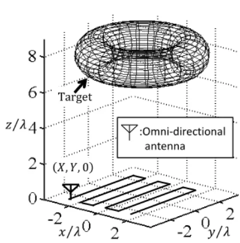
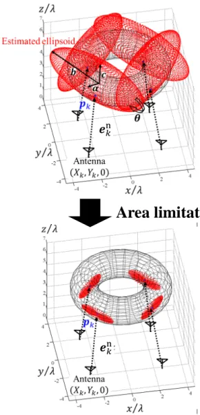
Figure 1 shows the system model. An omni-directional antenna is scanned on the x-y plane, where each location is defined as (X, Y,0). The mono-static radar is assumed. The transmitted signal as current source is defined as mono-cycle pulse with center wavelengthλ. It assumes the multiple linear polarizations for the xandy directions in transmitting and receiving, respectively. s′_i,j(X, Y, t) denotes the received electric field at the location (X, Y,0), at time t, when the transmitting and receiving polarization are along the i(xory) axis andj(xory) axis, respectively.s˜i,j(X, Y, t)is the output of the Wiener filter ofs′_i,j(X, Y, t)calculated as;

˜

si,j(X, Y, t) =

∫ _∞

−∞

W(ω)S_i,j′ (X, Y, ω)ejωtdω, (1) whereS′_i,j(X, Y, ω)is the signal in the frequency domain of s′_i,j(X, Y, t).W(ω)is defined as W(ω) = Sref(ω) ∗ (1−η)S2 0+η|Sref(ω)|2 S0, (2) whereη= 1/(1 + (S/N)−1₎_{, and}_S

ref(ω)is the reference

sig-nal in the frequency domain, which is the complex conjugate of that of the transmitted signal.S0is a constant for dimension

consistency. This filter is an optimal MSE (Mean Square Error) linear filter for additive noises. ˜si,j(X, Y, t)is now converted tosi,j(X, Y, R)usingR= ct/2λ, wherecis the speed of the radio wave. The range point extracted from the local maxima of sx,x(X, Y, R) as to R is denoted as q = (X, Y, R); the details are given in [8].

III. RPM METHOD ANDCONVENTIONALEXPANSION APPROACH

A. Original RPM method

We have already established accurate and high-speed 3-D target boundary extraction method as RPM method, which

⁄ ⁄ ⁄ Target :Omni-directional antenna , , 0

Fig. 1. System model.

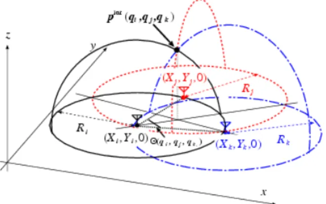
can be applicable to various 3-D target shapes having such as concave surface, edges ridges with 1/100 wavelength accuracy [8], [9]. the RPM method method is based on the assumption that a target boundary point(x, y, z) exists on a sphere with its center as the antenna location (X, Y,0) and its radius as the observed rangeR. The direction of arrival DOA for each range pointqi= (Xi, Yi, Ri), can be determined by assessing the spatial accumulation of intersection points of the spheres, whose center is(Xi, Yi,0)and radius isRi. The RPM method determines the target point for range pointq_i as:

ˆ p(qi) = arg max pint₍_q i;ql,qm)∈Pi ∑ (q_j,q_k)_∈Qi g(qi;qj,qk) ×exp { −∥p int_(q i;qj,qk)−pint(qi;ql,qm)∥2 2σ2 r } , (3) where pint_(q

i;qj,qk) denotes the intersection point among the three spheres, determined by the range points q_i, q_j and q_k. σr is an empirically determined constant. Figure 2 presents the spatial relationship between the three spheres with q_i,q_j, q_k and its intersection point. The weighting function g(q_i;q_j,q_k)is defined by: g(q_i;q_j,q_k) = s(q_j) exp { −D ( qi,qj )2 2σ2 D } +s(q_k) exp { −D(qi,qk) 2 2σ2 D } ,(4) wheres(q_j) denotes the amplitude ofs(q_j) at R=Rj and D(q_i,q_j) =√(Xi−Xj)2+ (Yi−Yj)2 hold. Eq. (4) yields the convergence effect of intersection points with respect to the antenna locations. A set of intersection points as Pi is defined as ; Pi = { pint(q_i;q_j,q_k)|(q_j,q_k)∈ Qi } . (5)

Qi denotes the investigating region of antenna locations. Note that, each target point regarded denote as p(qˆ i) is associated with each range pointqi, which means the one-to-one correspondence between them. While the RPM method accomplishes an accurate and fast 3-D imaging, even in richly

(4)

Fig. 2. Relationship among three spheres determined byqi,qj,qkand its

intersection point.

interfered situation caused by multiple target reflection or noisy environment, it (also SAR or others) suffers from an insufficient imaging region, when the aperture size is small. This insufficiency is an essential problem in radar imaging methods, and should be resolved by other approaches, such as an expansion schemes.

B. Single ellipsoid based expansion method

Here we briefly introduce the imaging method conven-tionally used to expand target image regions [14], which is based on an ellipse expansion of an image obtained by RPM. the method [14] performs ellipse fitting in the data space comprising the antenna location and observed range, which is enabled by the unique feature of RPM imaging [8]. Ellipse fitting of the RPM image in real space is overly sensitive to errors introduced by the RPM imaging process. In contrast, ellipse fitting in data space is essentially impervious to imaging error because the fitting process is directly carried out without through the imaging process, whereas RPM is only employed in image clustering. More specified, the method [14] first uses the target points produced by RPM only for the clustering of the range points, the distribution of which in data space is often very complicated in the case of multiple targets. The clustered range points are then employed for ellipse fitting, which is converted in data space. However, the method [14] assumes that the target is shaped similarly to an ellipse and is inaccurate for significantly dissimilar shapes. The applicability for non-ellipsoidal target, such as target with edge or having multiple reflection points has been also demonstrated[8], where the fatal inaccuracy for expansion has been confirmed. This is natural because of a simple assumption that target should be expressed as a “single “ ellipsoid. In addition, multiple targets or complicated target shapes must be correctly clustered; otherwise serious expansion error occurs.

IV. PROPOSEDMETHOD

This section proposes a novel method that exploits the fully polarimetric data, expanding RPM images to variously shaped targets and thereby solving the above-mentioned problem. In many studies, significant information on a target structure or

-2-0.5 0 0.5 -0.5 0 0.5 0 0.5 1 1.5 ⁄ _Target 0 ⁄ ⁄ 0 0 -2 2 -2 2 2 4 6 ࢇ ࢈ ࢉ ࣂ Antenna 0,0,0

Fig. 3. Observation model for fully polarimetric analysis to a single ellipsoid target.

condition has been obtained by analyzing or decomposing multiple polarimetric SAR images [17], [19], [20]. Thus, the potential of utilizing fully polarimetric data in object or scene detection is well recognized. This paper focuses on the image expansion issue for the reconstructed RPM image, by extracting the polarimetric feature through the time-series data based neural network learning and appropriate fitting algorithm for non-ellipsoidal shape target.

A. Polarimetric analysis for single ellipsoid target

We first investigate the relationship between the time-series waveform of the fully polarimetric data and ellipsoid param-eters (axial radius and rotation angle). Figure 3 shows the observation model that is subjected to polarimetric analysis. The target is assumed to be a single ellipsoid centered at (0,0, zc). The antenna is located at (0,0,0). Here, a, b and c are the radii of the ellipsoid along the x-axis, y-axis and z-axis, respectively, and θ is the rotation angle about the z -axis. The observation data are generated by the FDTD method. Figure 4 shows the Wiener filter output of the received signals sx,x,sx,y andsy,y in the time domain, where the parametera is varied while other parameters are fixed (b= 1.0λ,c= 0.5λ andθ= 0◦). In this figure, the amplitudes ofsx,xandsy,yare positively correlated with the axial radius a of the ellipsoid, while that of sx,y does not significantly change with axial radius. This fact demonstrates that the amplitude of polarized data along the major axis of an ellipsoid is directly related to an expansion for ellipsoid, where the x-y polarized data does not affect significantly, and this indicates that sx,x and sy,y contributes the size estimation of target shape. Figure 5 shows the Wiener filter output of the received signalsx,ywhen θ is varied and the other parameters are fixed as a = 3.0λ,

(5)

4.5 5 5.5 6 4.5 5 5.5 6 -0.4 -0.2 0 0.2 4.5 5 5.5 6 -0.4 -0.2 0 0.2 ⁄ ⁄ A m p li tu d e o f ݏ , 0.5 1.5 2.5 ⁄ A m p li tu d e o f ݏ , A m p li tu d e o f ݏ , 0 2 10ିଷ 2 10ିଷ

Fig. 4. Outputs of the Wiener filter sx,x(0,0, R), sx,y(0,0, R), and sy,y(0,0, R)whenais variable and other parameters are fixed asb= 1λ, c= 0.5λandθ= 0◦. 4.5 5 5.5 6 6.5 7 -0.02 -0.01 0 0.01 0.02

⁄

0° 20° 40° 20° 40° A m p li tu d e o f

ݏ

,

Fig. 5. Outputs of the Wiener filter sx,y(0,0, R) whenθis variable and

other parameters are fixed asa= 3λ,b= 2λandc= 0.5λ.

b= 2.0λandc= 0.5λ. Figure 5 also shows that an amplitude ofsx,y data significantly increases according to target rotation to maximum at 45◦. The received amplitude ofsx,y strongly correlates with the rotation angle; moreover, the sign of the phase indicates the rotation direction. Therefore, the rotation angle of the ellipsoid can be estimated from the sx,y signal. The fully polarimetric data, especially those of the time-series waveform, contain important information on both the local structure and global expanse of the target shape. Then, one RPM imaging point with no size can be expanded by partial ellipsoidal surface if such information can be extracted by fully polarimetric data. A m p li tu d e o f , , , ⁄ 1 ∆ 1∆ 1∆ ⁄ ⁄ A m p li tu d e o f , , , A m p li tu d e o f , , , 4.5 5 5.5 6 -0.2 0 0.2 4.5 5 6 -0.2 0 0.2 5.5

Fig. 6. Extraction scheme for time-series data in the proposed method.

ܽ

ܾ

ߠ

/ŶƉƵƚůĂǇĞƌ ,ŝĚĚĞŶůĂǇĞƌ ̃_,,

呍

̃ ,,

呍

̃_,,

呍

̃ ,, ̃_,, ̃_,, KƵƚƉƵƚůĂǇĞƌ K Ƶ ƚƉƵ ƚ

ܿ

呍

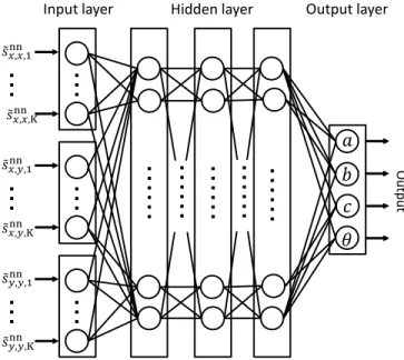
Fig. 7. Layer structure of neural network in the proposed method.

B. Neural network learning for fully polarimetric data

Based on previous analysis, the proposed method first prepares a time-series dataset of various ellipsoids with theira, b,c andθparameters. These parameters make important role in the expansion process, because the proposed method relies on the expansion with an aggregation of ellipsoid. Thus, a full polarimetric data for each range point needs to be associated with ellipsoid, the part of which expresses the local boundary of actual object. In this method, such association has been achieved via neural network based training process as follows.

(6)

Note that, when one considers a reflection data from ellipsoid object, there is a creeping wave propagating along backside of object. However, the strength of this component is much smaller than that of direct reflection, e.g. specular reflection, then, we deal with the time-series data with a finite length. To generate the input data for the windowed time-series data, we defined an input vector snn

i,j(X, Y, R)(i =x, y, j = x, y) for each range pointq= (X, Y, R):

snni,j(X, Y, R) ≡ [si,j(X, Y, R), si,j(X, Y, R+ ∆R), · · ·, si,j(X, Y, R+ (K−1)∆R)] (6) where ∆R corresponds to the time window scale, and K is a constant natural number. Figure 7 shows the structure of the neural network. In the training sequence, the input data of the received signal of the antenna located at(0,0,0), namely, (X, Y) = (0,0) are used, for simplicity, where the ellipsoid parameters(a, b, c, θ)are varied.

These parameters significantly depend on the amplitude of the input signal. Therefore, when inputting the received data into the trained neural network, the propagation attenuation of the received amplitude must be considered, because the amplitude directly affects the size of ellipsoid in the proposed method. The proposed method compensates for the propaga-tion attenuapropaga-tion of each received signal by applying a funcpropaga-tion of the measured range R. Theoretically, the amplitude of a signal radiated from a point source is attenuated on the first order of the propagation range. However, in this case, we must consider the reflection signals from various shape of target, and it is generally difficult to estimate an attenuation ratio without knowledge of target shape, theoretically. To address this problem, we investigated the attenuation ratios from various ellipsoids at various distances and calculated the average attenuation ratio. Specifically, the distance from an ellipsoid target to the antenna was rescaled as 1.0λ to 10λ in1.0λinterval. The antenna was located at(0,0,0), and the observation data are also generated by FDTD. The ellipsoid was postured as shown in Fig. 3. The ellipsoid parametersa,b andcare each varied as0.5λ,1λ,1.5λ,2λ,2.5λand3λ, while θ= 0◦ is fixed.

The input time-series data˜snn_i,j(X, Y, R)(i=x, y, j=x, y) are then compensated as

˜

snn_i,j(X, Y, R) =f(R/R0)snni,j(X, Y, R0) (7)

wheref(R/R0)denotes the averaged attenuation ratio andR0

is the reference distance. Note that, f(R/R0)is a polynomial

function of R/R0, which is fitted to the logarithm of the

above-described dataset.

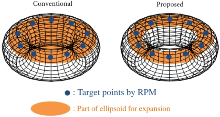
C. Multiple ellipsoids based image expansion for RPM point

Our image expansion methodology relies on fitting each RPM target point to a partial ellipsoidal surface with param-eters estimated by the above neural network approach. In the literature [14], each group of target points obtained by RPM was expanded as a single ellipsoid, which is problematic for shapes that widely differ from ellipsoids. Thus, the proposed method expresses each RPM target point as part of an ellipsoid surface; that is, a single target shape is expressed as an

Conventional Proposed

: Target points by RPM : Part of ellipsoid for expansion

Fig. 8. Scheme comparison between the conventional and the proposed methods.

aggregation of partial ellipsoidal surfaces. Figure 8 shows the difference between the conventional and the proposed schemes for image expansion. In this sense, our method differs from that of [14]. Figure 9 illustrates the basic concept of the multiple ellipsoid-based expansion scheme. In the proposed method, the part of each ellipsoid (estimated by each q_k through the trained neural network) is fitted to each RPM point as p_k, using LOS directionen_k. Note that, to avoid an over-fitting, only the portion of ellipsoid is used for image expansion.

For appropriate fitting the partial ellipsoid, the ellipsoid boundary points are converted to fit the RPM point and its LOS direction as;

  x E k yE k zE k   = 

 cos ˆsin ˆθθ −cos ˆsin ˆθθ 00

0 0 1

 



 ˆaˆ_bcos_cosϕ_ϕcos_sin_ψψ ˆ csinψ   +   00 Rk−(zc−ˆc/2)   (8)

where(ˆa,ˆb,ˆc,θˆ)is estimated parameters for the range points qk, and ϕ and ψ are azimuthal and elevation angles of the ellipsoid, respectively. To determine the ellipsoid for each target point, we need to estimate the 9 degree of freedom. In this case, we investigate 4 independent parameters a,b,c andϕ, and need to determine other 5 parameters from RPM point and its geometrical characteristic. Here, applying RPM to the range points q_k = (Xk, Yk, Rk), we also estimated a corresponding target point p_k = (xk, yk, zk) . Note that each target point p_k satisfies a one-to-one correspondence with each range point q_k; this feature is unique to RPM imaging. Under the assumption that the antenna receives a strong echo from the target boundary, which is perpendicular to the line of sight (LOS) direction on p_k, the unit vector of the LOS direction, that is, normal vector on target boundary, is calculated asen,k = (pk−(Xk, Yk,0))/||pk−(Xk, Yk,0)||. In addition, since the target boundary should be tangent to the plane orthogonal to this normal vector, the expanding ellipsoid should also be tangent to the target boundary. Even in this geometrical condition, the total parameters of ellipsoid cannot be uniquely determined, then, for simplicity, we assume that

(7)

Area limitation

ࢋ

_௞୬

ࢋ

_௞୬

Fig. 9. Example of the expanded result by the proposed method.

the tangential point of each ellipsoid is located, at an elevation angle ψ=−π/2.

Then, the LOS direction in the learning process as in Fig. 3, namely,ez= (0,0,1), is converted to that for each range point q_k according to en

k. According to the conversion, each point (xE

k, yEk, zkE)on estimated ellipsoid boundary is also converted as;

(˜xE_k,y˜E_k,z˜_kE)T = Rk(erot_k , ξ_krot)(x_kE, y_kE, z_kE)T +(Xk, Yk,0)T, (9)

where the matrix Rk(erotk , ξ

rot

k ) denotes 3-dimensional rota-tion along the axis erot_k = ez×e

n

k |ez×en

k|

with the angle ξrot_k =

Fig. 10. Ellipsoid rotation and translation along the LOS directionen_k.

, Δ, 0 , 0 a , Δ, Δ Δ, 0 , 0 b Δ, Δ :Reflection point

Fig. 11. Relationship between∆x/∆Xand curvature on target surface. cos−1(ez·en_k). Specifically, the matrix is calculated as;

Rk(erot_k , ξ_krot) =

  Ck(e rot x,k) 2_{+ cos}_ξrot k Ckerotx,ke rot y,k−e rot z,ksinξ rot k Ckerotz,ke rot x,k−e rot y,ksinξ rot k Ck(eroty,k) 2_{+ cos}_ξrot k Ckerotz,ke rot x,k−e rot y,ksinξ rot k Ckeroty,ke rot z,k+e rot x,ksinξ rot k (10) Ckerotz,ke rot x,k+e rot y,ksinξ rot k Ckeroty,ke rot z,k−e rot x,ksinξ rot k Ck(erotz,k) 2_{+ cos}_ξrot k  ,

whereerot_k = (erot_x,k, erot_y,k, erot_z,k)and Ck = 1−cosξrotk . Figure 10 illustrates the translation and rotation of the ellipse so as to fit the target pointpk.

Finally, a part of ellipsoid is extracted as Ωkˆ for each q_k. To accomplish an edge preserving property in expansion process, the proposed method changes a size of portion of ellipsoid, corresponding to curvature radius on target surface. The literature [22] or [23] revealed that the following matrix can assess the curvature radius along each axis;

Sk =    ∂xk ∂Xk ∂yk ∂Xk ∂xk ∂Yk ∂yk ∂Yk   ≃    ∆xk ∆Xk ∆yk ∆Xk ∆xk ∆Yk ∆yk ∆Yk   , (11)

(8)

where(xk, yk, zk)denotes the target boundary point estimated by RPM corresponding toq_k= (Xk, Yk, Rk). Note that, each difference approximation in the right term in Eq. 11 is readily calculated by using the one-to-one relationship between q_k and (xk, yk, zk). Figure 11 shows the relationship between object boundaries with small or large curvature radius, and the value of ∂yk/∂Xk in the two-dimensional view. As shown in Fig. 11, ∂yk/∂Xk can approximately and simply assess the curvature radius indirectly. Then, the parameter for expansion area is calculated as follows;

ϕk(ψ) =

√

uk(ψ)2₊_v

k(ψ)2ϕE (0≤ψ≤2π), (12)

(uk(ψ) vk(ψ) )T=Uk(λ1,kcos(ψ) λ2,ksin(ψ) )T, (13) where ψandϕk(ψ)denote the elevation and azimuth angles of an expanded ellipsoid, respectively. λ1,k and λ2,k are eigenvalues of Sk, which determine principal curvature on (xk, yk, zk), and Uk is the matrix consisted of eigenvecters of Sk. ψE is determined empirically. This process enables us to change an expansion area depending on its curvature, namely, an edge preserving is possible.

Then, the expanded image Ωˆex is determined as;

ˆ Ωex= ∪ k ˆ Ωk (14)

The lower side of Fig. 9 denotes the area limitation example, described above.

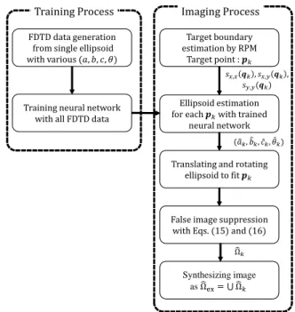
After training process through neural network with FDTD data, the actual imaging process in the proposed method is summarized as follows;

Step 1). Target boundary points p_k = (xk, yk, zk)(k = 1, ..., NRP) are obtained by applying the RPM to

q_k = (Xk, Yk, Rk)which is extracted from the local maximum ofsx,x(Xk, Yk, Rk).

Step 2). snn

i,j,k(X, Y, R) for qk (uniquely connected with p_k) are extracted as in Eq. (6), and are compensated as s˜nn_i,j,k(X, Y, R) in Eq. (7) corresponding to the observation distanceRk.

Step 3). s˜nn_i,j,k(X, Y, R) is inputted to the trained neural network for obtaining the parameters of ellipsoid as (ˆak,ˆbk,ˆck,θˆk).

Step 4). Each estimated ellipsoid denoted as(xE_k, y_kE, z_kE) is rotated and translated as (˜xE_k,y˜_kE,z˜E_k) so that it fits each target point pk = (xk, yk, zk) in Eq. (9), and its partial area asΩkˆ is extracted.

Step 6). For all range points q_k, Step 2) and Step 5) are carried out and generates an each expanded image as ˆ

Ωk.

Step 7). For the l th discrete member belonging in Ωˆk, denoted aspE

k,l, the following evaluation function is introduced; ζ(pE_k,l) = ∑ m,n,(m_̸=k) exp { −∥p E k,l−p E m,n∥2 2σ2 ζ } (15) If the following condition is satisfied;

ζ(pE_k,l)≤γmax m,nζ(p E m,n) (16) Target boundary estimation by RPM Target point : ௞ Ellipsoid estimation for each ௞ with trained

neural network

Translating and rotating ellipsoid to fit ௞

False image suppression with Eqs. (15) and (16)

Synthesizing image as Ωୣ୶ ⋃ Ω௞ ,, ,, , , , ̂, Ω FDTD data generation from single ellipsoid with various , , ,

Training neural network with all FDTD data

Training Process Imaging Process

Fig. 12. Flowchart of the proposed method.

The point pE_k,l is remove from Ωkˆ . Final expanded image Ωˆex is expressed as aggregate of Ωkˆ as in

Eq. (14).

Figure 12 outlines the flowchart of the proposed method. Note that, the post-procedure in Step 7) makes role of eliminat-ing the large deviated points in considereliminat-ing the spatial density of all expanded imaging points aspE_k,l. The parameterσζ can be determined by considering the assumed sampling interval of each discrete formed ellipsoid. As in this flowchart, once the NN learned the training data generated by the FDTD, the proposed method does not require the FDTD or NN training process for each imaging, which maintains the high-speed 3-D imaging with this method. In addition, the proposed method does not need any clustering scheme for RPM points in advance, which is required in [14]. This is because each ellipsoid is independently assigned to each target point.

V. PERFORMANCEEVALUATION INNUMERICAL SIMULATION

This section describes the two types of performance evalua-tions. One is the evaluation for neural network based learning using fully polarimetric data, where unknown parameters of ellipsoid are estimated by the neural network with time-series data base. The other demonstrates the performance of image expansion by our proposed method, namely, multiple ellipsoid based expansion for RPM imaging points.

A. Ellipsoid parameter estimation by neural network

This section reports on the parameter estimation of a single ellipsoid from the fully polarimetric dataset. The antenna is located at (x, y, z) = (0,0,0). During the learning stage of the neural network, the parameters a, b andc of the training

(9)

TABLE I

ESTIMATION RESULTS FOR THE NEURAL NETWORK BASED PARAMETER ESTIMATION OF SINGLE ELLIPSOID.

True Estimated Relative error

(a/λ,b/λ,c/λ,θ/deg) (a/λ,b/λ,c/λ,θ/deg) (a,b,c,θ)[%] (1.70,1.00,2.50,30.0) (1.72,0.97,2.51,28.0) (1.14,2.68,0.28,6.76) (1.50,2.20,3.00,20.0) (1.51,2.18,3.00,21.7) (0.85,0.73,0.05,8.53) (1.00,2.00,2.70,40.0) (1.01,2.01,2.69,43.2) (0.62,0.56,0.24,7.99) (2.00,1.50,1.00,-35.0) (2.02,1.48,0.97,-37.0) (0.97,1.48,3.48,5.39) (1.40,2.80,2.00,10.0) (1.40,2.82,2.01,9.6) (0.33,0.64,0.36,3.68) (2.30,1.50,1.10,20.0) (2.38,1.47,1.09,19.1) (3.39,2.18,1.07,4.34) (2.80,2.50,0.50,25.0) (2.64,2.67,0.53,20.7) (5.87,6.77,5.92,17.34) (3.00,1.70,0.90,30.0) (3.22,1.78,0.85,28.2) (7.48,4.97,5.27,6.15) (2.50,1.30,2.00,13.0) (2.53,1.32,2.04,14.0) (1.20,1.82,2.03,7.48) (1.00,2.00,2.40,-15.0) (1.02,2.01,2.39,-14.9) (1.76,0.67,0.22,0.55) (2.80,1.70,1.10,35.0) (2.81,1.74,1.16,36.6) (0.35,2.46,5.00,4.57)

ellipsoids are varied as 0.5λ,1λ,1.5λ,2λ,2.5λ and 3λ, and θ is varied as−40◦,−30◦,−20◦,−10◦,0◦,10◦,20◦,30◦ and 40◦, respectively. All of these a, b, c and θ namely, 1944 different combinations are used as the training data. The conductivity and relative permittivity of the ellipsoid target are set to1.0×107_S_/_m_and_ϵ_{= 1}_.₀_{, respectively. The observation}

data are generated by the FDTD method assuming a noiseless situation. The neural network contains three hidden layers, with 30 neurons in the first layer, 20 in the second layer, and 10 in the final layer. Here, K∆R = 1.44λ, and the sample interval of range as ∆R = 0.03λ are set in Eq. (6). Table I lists the parameters of the ellipsoid targets estimated by the trained neural network. The untrained parameters are depicted in red font. From Table I, it can be observed that the time-series based neural network accurately estimated the ellipsoidal parameters. The average relative errors in a, b, c andθ are2.7%,2.3%,1.3%and6.9%, respectively.

B. Expansion Performance

This subsection presents the expansion results of our pro-posed method. The transmitting and receiving antenna set is scanned over the area −2.5λ ≤ x, y ≤ 2.5λ at 0.5λ intervals in the x and y directions. Again, the observation data are generated by the FDTD method. Here, the operational frequency band (10dB criteria mostly used in UWB signal) in this simulation is about 2.0 GHZ, and its range resolution is 150 mm. The center frequency is 3 GHz, (corresponding wavelength in the air is 100mm), denoting that its fractional bandwidth is around 66 %.

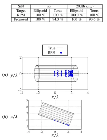
In RPM imaging, the set of range points q_x,x extracted by sx,x(X, Y, R′)is used only in the initial 3-D imaging. Figure 13 shows the target points obtained by RPM for the ellipsoid target, where the solid lines show the discrete expression of the true ellipsoidal boundary. Here,a= 2.5λ,b= 1.5λ,c= 1.0λ, θ = 0◦, and the y-axis is rotated through 20◦. According to Fig. 13, the target points obtained by RPM cannot sufficiently express target image to recognize the original ellipsoidal shape, while highly reconstruction accuracy is provided. This is because the target is located from sensor location with significant distance around 6λ, and this leads to smaller aperture angle. On the contrary, Fig. 14 shows the image

expansion result obtained by the proposed method. Here, the elevation angle of each ellipsoid is limited to(ϕE =−7π/18). Also, the parameter σζ = 0.25λandγ = 0.3 in Eq. (15) are set. Figure 14 indicates that the proposed method correctly expands the target points obtained from the RPM imaging points. Figures 15 and 16 show the target points obtained by RPM and the expansion expression of the proposed method, respectively. The target is the torus shown in Fig. 1. According to these figures, the proposed method significantly enhances the imaging region of the torus boundary, which is dissimilar to an ellipsoid. The expansion errors in Fig. 16 result from the inaccurate estimation of the ellipsoid parameters from time-series data, because each antenna receives multiple reflection echoes within range resolution from the torus boundary, and then, the expansion accuracy depends on the operational bandwidth, naturally. It should be considered that an another cause is the convex boundary based fitting with ellipsoid, namely, the positive principal curvature, while the part of torus boundary has a negative principal curvature, such as saddle boundary. However, a largely deviated artifact of the part of expansion image is efficiently suppressed by introducing the post-processing denoted in Step 7) in the proposed method. It should be also noted that there is accuracy degradation caused by the discrepancy between the reference signal and actual received signal in ranging process with Wiener filtering. However, such kind of ranging inaccuracy is the order of0.1λ, and affects both RPM and the proposed methods [21], [22]. To prevent this interference effect, the windowing time span for extracting the time series data should be also appropriately determined. The average calculation times for the original RPM and the proposed method after NN learning, are 0.2 sec and 30 sec, respectively, using Intel Xeon CPU E5-1620 v2 3.70 GHz processor, and such calculation time is hardly achieved by the conventional beamforming or Kirchhoff migration algorithms in obtaining the 3-D full image.

We now discuss a noisy situation. Each received signal is subjected to Gaussian white noises sx,x, sx,y and sy,y. The signal-to-noise ratio S/N is defined as the ratio of the peak instantaneous signal power in all polarization data to the average noise power after applying a matched filter. Figure 18 shows the RPM-obtained target points of a single ellipsoid in the noisy case. The average S/N ofsx,yis approximately 20 dB and those ofsx,x andsy,y are approximately 50 dB. It should be noted that the above definition is the most strict estimation for S/N, because the matched filter is most noise-robust filter, namely this definition considers the locality of signal in both time and frequency domain. Figure 17 shows an example of received signals assuming S/N=20dB, and it denotes that while signal can be recognized after applying matched filter (denoted as (c)), the raw received signal (b) (before applying matched filter) is more noisy. Such S/N level signal is usually obtained in the real experiment assuming short range sensing (distance from sensor is within 5m), as demonstrated in [10].

Figure 18 indicates that the RPM retains sufficient accuracy even in a noisy situation, while the estimated points expresses only a portion of the whole target shape. Figure 19 shows the expansion results of the proposed method. Although the expansion accuracy is slightly worse than that in the

(10)

noise-⁄ ⁄ ⁄ ⁄ True RPM

Fig. 13. Target boundary points estimated by RPM method for single ellipsoid target in noiseless situation (a: projection tox-y plane,b: cross-section for

y=0 plane.). Solid lines show the discrete expression of true boundary.

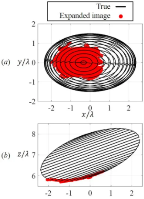
Fig. 14. Expansion result of the proposed method for single ellipsoid target in noiseless situation (a: projection to x-y plane,b: cross-section fory=0 plane.). Solid lines show the discrete expression of true boundary.

less situation, the proposed method significantly expanded the region that can be imaged, while maintaining acceptable accuracy. Figs. 20 and 21 show the results of imaging a torus by RPM and by the proposed expansion method, respectively. The approximate average S/N of sx,y, sx,x and sy,y are 20 dB, 32 dB, and 32 dB, respectively. Comparing these results to the noiseless case, the noise did not severely degrade the image expansion, and the expansion of the image is retained. Finally, the image expansion is quantitatively analyzed

True RPM ⁄ ⁄ ⁄ ⁄

Fig. 15. Target boundary points estimated by RPM method for torus target in noiseless situation (a: projection tox-y plane, b: cross-section fory=0 plane.). Solid lines show the discrete expression of true boundary.

Fig. 16. Expansion result of the proposed method for torus target in noiseless situation (a: projection tox-yplane,b: cross-section fory=0 plane.). Solid lines show the discrete expression of true boundary.

by investigating the effective reconstruction image region, namely, the expansion effect. For this evaluation, first, a whole true target boundary denoted as Ωtrue

all is divided into small

regions with the same area as∆Ωtrue

i ,(i= 1,2,· · ·, Ntar). A

whole target boundary region is expressed as Ωtrue_all =∪

i

∆Ωtrue_i . (17)

Also, the center point for the regionΩtrue_i is defined asptrue_i . Then, for the k-th estimated target point denoted as pest

(11)

400 600 800 1000 1200 1400 1600 time -1 0 1 am p li t u de (a) (b) (c)

Received signal in noiseless case

Output of matched filter at S/N=20dB Received signal at S/N=20dB

Time

Fig. 17. Example of received signal. (a): Received signal in noiseless case. (b): Received signal in S/N=20dB. (c): Output of matched filter for received signal illustrated in (b). ⁄ ⁄ ⁄ ⁄ True RPM

Fig. 18. Target boundary points estimated by RPM method for ellipsoid target in S/N=20dB (a: projection tox-y plane,b: cross-section fory=0 plane.). Solid lines show the discrete expression of true boundary.

estimated effective image areaΩˆeﬀ

k is defined as; ˆ Ωeﬀ_k = { ∪ i

∆Ωtrue_i ∥ptrue_i −pest_k ∥ ≤δp

}

, (18)

where δp is threshold for extracting effective image region, which is empirically determined as δp = 0.2λ, in this case. The effective image areaΩêff composed of all target points is defined as; ˆ Ωeff =∪ k ˆ Ωeffk . (19)

As the evaluation value for image expansion effect, the image

Fig. 19. Expansion result of the proposed method for ellipsoid target in S/N=20dB (a: projection tox-yplane,b: cross-section fory=0 plane.). Solid lines show the discrete expression of true boundary.

TABLE II

VALUE OFPa[%]OF EACH METHOD.

S/N ∞ 20dB(sx,y)

Target Ellipsoid Torus Ellipsoid Torus

RPM 15.9 % 7.2 % 16.3 % 7.6 %

Proposed 21.6 % 34.9 % 26.7 % 35.4 %

expansion ratio is defined as; Pa=

Seﬀ

Strue

, (20)

where Strue and Seﬀ denote the areas of Ωtrueall and Ωˆ eﬀ_,

respectively. Figure 22 illustrates for the effective image area ˆ

Ωeﬀ_k for each target pointpest_k . The percentage image expan-sion ratioPain the absence and presence of noise is computed

for each method, and the results are summarized in Table II. Clearly, the proposed method significantly expands the target image, even when the target deviated from an ellipsoid.

However (see also Figs. 16 and 21), in the case of torus shaped target, there are non-negligible errors in expansion. Although it significantly enhances the image expansion ratio, expansion accuracy requires an additional evaluation criterion. The error in the image reconstruction is given by

e(pest_k )≡min p_truep

est

k −p

true ₍_k_{= 1}_,₂_{, . . . , N}

est), (21)

whereptrue _{denotes the true target points in discrete}

expres-sion with sufficiently dense sample andNest denotes the total

number of the estimated points. Figures 23 and 24 plot the number of estimated points with error e(pest_k ) in expansions of ellipsoidal and toroidal targets, respectively. While the proposed method and RPM yield the same reconstruction accuracy of ellipsoidal targets, RPM better reconstructs the toroidal target, because of the aforementioned interference

(12)

True RPM ⁄ ⁄ ⁄ ⁄

Fig. 20. Target boundary points estimated by RPM method for torus target in S/N=20dB (a: projection tox-y plane,b: cross-section fory=0 plane.). Solid lines show the discrete expression of true boundary.

Fig. 21. Expansion result of the proposed method for torus target in S/N=20dB (a: projection tox-yplane,b: cross-section fory=0 plane.). Solid lines show the discrete expression of true boundary.

effect in the proposed method. However, the maximum error in the toroidal target is within 1λ, and the apparent expanded image does not markedly deviate from the actual target shape. Table III lists the percentage of estimated target points satisfy-inge(pest

k )≤0.2λin the ellipsoidal and toroidal cases. Com-bining this evaluation and the image expansion ratio denoted as Pa shown in Table II, the proposed method achieves an effective target image expansion without sacrificing a serious accuracy degradation. Clearly, the percentage of accurately estimated target points (expanded points) is reduced when our method is applied to toroidal objects. This inaccuracy must be addressed in our future work.

00000000000000000000000000000000000000000000000000000000000000000000000000000000000000000000000000000000000000000000000000000000000000000000000000000000000000000000000 00000000000000000000000000000000000000000000000000000000000000000000000000000000000000000000000000000000000000000000000000000000000000000000000000000000000000000000000 00000000000000000000000000000000000000000000000000000000000000000000000000000000000000000000000000000000000000000000000000000000000000000000000000000000000000000000000 00000000000000000000000000000000000000000000000000000000000000000000000000000000000000000000000000000000000000000000000000000000000000000000000000000000000000000000000 00000000000000000000000000000000000000000000000000000000000000000000000000000000000000000000000000000000000000000000000000000000000000000000000000000000000000000000000 00000000000000000000000000000000000000000000000000000000000000000000000000000000000000000000000000000000000000000000000000000000000000000000000000000000000000000000000 00000000000000000000000000000000000000000000000000000000000000000000000000000000000000000000000000000000000000000000000000000000000000000000000000000000000000000000000 00000000000000000000000000000000000000000000000000000000000000000000000000000000000000000000000000000000000000000000000000000000000000000000000000000000000000000000000 00000000000000000000000000000000000000000000000000000000000000000000000000000000000000000000000000000000000000000000000000000000000000000000000000000000000000000000000 00000000000000000000000000000000000000000000000000000000000000000000000000000000000000000000000000000000000000000000000000000000000000000000000000000000000000000000000 00000000000000000000000000000000000000000000000000000000000000000000000000000000000000000000000000000000000000000000000000000000000000000000000000000000000000000000000 00000000000000000000000000000000000000000000000000000000000000000000000000000000000000000000000000000000000000000000000000000000000000000000000000000000000000000000000 00000000000000000000000000000000000000000000000000000000000000000000000000000000000000000000000000000000000000000000000000000000000000000000000000000000000000000000000 0000000000000000000000000000000000000000000000000000000000000000000000000000000000000000000000000000000000000000000000000000000000000000000000000000000000000000000000 0000000000000000000000000000000000000000000000000000000000000000000000000000000000000000000000000000000000000000000000000000000000000000000000000000000000000000000000 0000000000000000000000000000000000000000000000000000000000000000000000000000000000000000000000000000000000000000000000000000000000000000000000000000000000000000000000 0000000000000000000000000000000000000000000000000000000000000000000000000000000000000000000000000000000000000000000000000000000000000000000000000000000000000000000000 0000000000000000000000000000000000000000000000000000000000000000000000000000000000000000000000000000000000000000000000000000000000000000000000000000000000000000000000 0000000000000000000000000000000000000000000000000000000000000000000000000000000000000000000000000000000000000000000000000000000000000000000000000000000000000000000000 0000000000000000000000000000000000000000000000000000000000000000000000000000000000000000000000000000000000000000000000000000000000000000000000000000000000000000000000 0000000000000000000000000000000000000000000000000000000000000000000000000000000000000000000000000000000000000000000000000000000000000000000000000000000000000000000000 0000000000000000000000000000000000000000000000000000000000000000000000000000000000000000000000000000000000000000000000000000000000000000000000000000000000000000000000 0000000000000000000000000000000000000000000000000000000000000000000000000000000000000000000000000000000000000000000000000000000000000000000000000000000000000000000000 0000000000000000000000000000000000000000000000000000000000000000000000000000000000000000000000000000000000000000000000000000000000000000000000000000000000000000000000 0000000000000000000000000000000000000000000000000000000000000000000000000000000000000000000000000000000000000000000000000000000000000000000000000000000000000000000000 0000000000000000000000000000000000000000000000000000000000000000000000000000000000000000000000000000000000000000000000000000000000000000000000000000000000000000000000 00000000000000000000000000000000000000000000000000000000000000000000000000000000000000000000000000000000000000000000000000000000000000000000000000000000000000000000000 00000000000000000000000000000000000000000000000000000000000000000000000000000000000000000000000000000000000000000000000000000000000000000000000000000000000000000000000 00000000000000000000000000000000000000000000000000000000000000000000000000000000000000000000000000000000000000000000000000000000000000000000000000000000000000000000000 00000000000000000000000000000000000000000000000000000000000000000000000000000000000000000000000000000000000000000000000000000000000000000000000000000000000000000000000 00000000000000000000000000000000000000000000000000000000000000000000000000000000000000000000000000000000000000000000000000000000000000000000000000000000000000000000000 00000000000000000000000000000000000000000000000000000000000000000000000000000000000000000000000000000000000000000000000000000000000000000000000000000000000000000000000 00000000000000000000000000000000000000000000000000000000000000000000000000000000000000000000000000000000000000000000000000000000000000000000000000000000000000000000000 00000000000000000000000000000000000000000000000000000000000000000000000000000000000000000000000000000000000000000000000000000000000000000000000000000000000000000000000 00000000000000000000000000000000000000000000000000000000000000000000000000000000000000000000000000000000000000000000000000000000000000000000000000000000000000000000000 00000000000000000000000000000000000000000000000000000000000000000000000000000000000000000000000000000000000000000000000000000000000000000000000000000000000000000000000 00000000000000000000000000000000000000000000000000000000000000000000000000000000000000000000000000000000000000000000000000000000000000000000000000000000000000000000000 00000000000000000000000000000000000000000000000000000000000000000000000000000000000000000000000000000000000000000000000000000000000000000000000000000000000000000000000 00000000000000000000000000000000000000000000000000000000000000000000000000000000000000000000000000000000000000000000000000000000000000000000000000000000000000000000000 00000000000000000000000000000000000000000000000000000000000000000000000000000000000000000000000000000000000000000000000000000000000000000000000000000000000000000000000 00000000000000000000000000000000000000000000000000000000000000000000000000000000000000000000000000000000000000000000000000000000000000000000000000000000000000000000000 00000000000000000000000000000000000000000000000000000000000000000000000000000000000000000000000000000000000000000000000000000000000000000000000000000000000000000000000 00000000000000000000000000000000000000000000000000000000000000000000000000000000000000000000000000000000000000000000000000000000000000000000000000000000000000000000000 00000000000000000000000000000000000000000000000000000000000000000000000000000000000000000000000000000000000000000000000000000000000000000000000000000000000000000000000 00000000000000000000000000000000000000000000000000000000000000000000000000000000000000000000000000000000000000000000000000000000000000000000000000000000000000000000000 00000000000000000000000000000000000000000000000000000000000000000000000000000000000000000000000000000000000000000000000000000000000000000000000000000000000000000000000 00000000000000000000000000000000000000000000000000000000000000000000000000000000000000000000000000000000000000000000000000000000000000000000000000000000000000000000000 00000000000000000000000000000000000000000000000000000000000000000000000000000000000000000000000000000000000000000000000000000000000000000000000000000000000000000000000 00000000000000000000000000000000000000000000000000000000000000000000000000000000000000000000000000000000000000000000000000000000000000000000000000000000000000000000000 00000000000000000000000000000000000000000000000000000000000000000000000000000000000000000000000000000000000000000000000000000000000000000000000000000000000000000000000 00000000000000000000000000000000000000000000000000000000000000000000000000000000000000000000000000000000000000000000000000000000000000000000000000000000000000000000000 00000000000000000000000000000000000000000000000000000000000000000000000000000000000000000000000000000000000000000000000000000000000000000000000000000000000000000000000 00000000000000000000000000000000000000000000000000000000000000000000000000000000000000000000000000000000000000000000000000000000000000000000000000000000000000000000000 00000000000000000000000000000000000000000000000000000000000000000000000000000000000000000000000000000000000000000000000000000000000000000000000000000000000000000000000 00000000000000000000000000000000000000000000000000000000000000000000000000000000000000000000000000000000000000000000000000000000000000000000000000000000000000000000000 00000000000000000000000000000000000000000000000000000000000000000000000000000000000000000000000000000000000000000000000000000000000000000000000000000000000000000000000 00000000000000000000000000000000000000000000000000000000000000000000000000000000000000000000000000000000000000000000000000000000000000000000000000000000000000000000000 00000000000000000000000000000000000000000000000000000000000000000000000000000000000000000000000000000000000000000000000000000000000000000000000000000000000000000000000 00000000000000000000000000000000000000000000000000000000000000000000000000000000000000000000000000000000000000000000000000000000000000000000000000000000000000000000000 00000000000000000000000000000000000000000000000000000000000000000000000000000000000000000000000000000000000000000000000000000000000000000000000000000000000000000000000 00000000000000000000000000000000000000000000000000000000000000000000000000000000000000000000000000000000000000000000000000000000000000000000000000000000000000000000000 00000000000000000000000000000000000000000000000000000000000000000000000000000000000000000000000000000000000000000000000000000000000000000000000000000000000000000000000 00000000000000000000000000000000000000000000000000000000000000000000000000000000000000000000000000000000000000000000000000000000000000000000000000000000000000000000000 00000000000000000000000000000000000000000000000000000000000000000000000000000000000000000000000000000000000000000000000000000000000000000000000000000000000000000000000 00000000000000000000000000000000000000000000000000000000000000000000000000000000000000000000000000000000000000000000000000000000000000000000000000000000000000000000000 00000000000000000000000000000000000000000000000000000000000000000000000000000000000000000000000000000000000000000000000000000000000000000000000000000000000000000000000 00000000000000000000000000000000000000000000000000000000000000000000000000000000000000000000000000000000000000000000000000000000000000000000000000000000000000000000000 00000000000000000000000000000000000000000000000000000000000000000000000000000000000000000000000000000000000000000000000000000000000000000000000000000000000000000000000 00000000000000000000000000000000000000000000000000000000000000000000000000000000000000000000000000000000000000000000000000000000000000000000000000000000000000000000000 00000000000000000000000000000000000000000000000000000000000000000000000000000000000000000000000000000000000000000000000000000000000000000000000000000000000000000000000 00000000000000000000000000000000000000000000000000000000000000000000000000000000000000000000000000000000000000000000000000000000000000000000000000000000000000000000000 00000000000000000000000000000000000000000000000000000000000000000000000000000000000000000000000000000000000000000000000000000000000000000000000000000000000000000000000 00000000000000000000000000000000000000000000000000000000000000000000000000000000000000000000000000000000000000000000000000000000000000000000000000000000000000000000000 00000000000000000000000000000000000000000000000000000000000000000000000000000000000000000000000000000000000000000000000000000000000000000000000000000000000000000000000 00000000000000000000000000000000000000000000000000000000000000000000000000000000000000000000000000000000000000000000000000000000000000000000000000000000000000000000000 00000000000000000000000000000000000000000000000000000000000000000000000000000000000000000000000000000000000000000000000000000000000000000000000000000000000000000000000 ௜ ୲୰୳ୣ ௞ ୣୱ୲ 000000000000000000000000000000000000000000000000000000000000000000000000000000000000000 000000000000000000000000000000000000000000000000000000000000000000000000000000000000000 000000000000000000000000000000000000000000000000000000000000000000000000000000000000000 000000000000000000000000000000000000000000000000000000000000000000000000000000000000000 000000000000000000000000000000000000000000000000000000000000000000000000000000000000000 000000000000000000000000000000000000000000000000000000000000000000000000000000000000000 000000000000000000000000000000000000000000000000000000000000000000000000000000000000000 000000000000000000000000000000000000000000000000000000000000000000000000000000000000000 000000000000000000000000000000000000000000000000000000000000000000000000000000000000000 ௜ିଵ ୲୰୳ୣ ௜ାଵ ୲୰୳ୣ

: Ω

௞ ୣ୤୤ ΔΩ௜ିଵ ୲୰୳ୣ ΔΩ௜ ୲୰୳ୣ ΔΩ௜ାଵ ୲୰୳ୣ

Fig. 22. Spatial relationship of effective image areaΩˆeﬀ

k for each target point pest

k .

Fig. 23. Number of the estimated target points of ellipse target in noiseless and noisy situation.

Fig. 24. Number of the estimated target points of torus target in noiseless and noisy situation.

C. Evaluation for edge preserving property

To demonstrate the edge preserving property of the proposed method, this section introduces the example for cylinder shape target. Figures 25 and 26 show the RPM-obtained target points and the expanded image by the proposed method, respectively. A noiseless situation is assumed. As shown in Fig. 25, the RPM holds a high accuracy even around the end of cylinder target, but expresses a part of cylinder shape. Figure 26 shows that our proposed method expands the cylinder shape without over expansion the edge region, where the expansion area is limited along a larger curvature direction in Eq. (13). The ratio

(13)

TABLE III

RATE OF ESTIMATED TARGET POINTS THAT SATISFY E≤0.2λ.

S/N ∞ 20dB(sx,y)

Target Ellipsoid Torus Ellipsoid Torus

RPM 100 % 100 % 100.0 % 100 % Proposed 100 % 94.3 % 100 % 90.6 % ⁄ ⁄ ⁄ ⁄ True RPM

Fig. 25. Target boundary points estimated by RPM method for cylinder target. Solid lines show the discrete expression of true boundary.

that the reconstructed points satisfies that the errors less than 0.2λ, are 100 % for both the conventional and the proposed methods. The image expansion ratios denoted asPaare 6.9% for the original RPM and 14.4%for the the proposed method, respectively. These quantitative evaluations also show that our method successfully expands the cylinder shape target, which guarantees an edge preserving property.

VI. CONCLUSION

This paper proposed a novel 3-D image expansion method that incorporates the RPM method but exploits the fully polarimetric dataset. In a time-series data analysis of fully polarimetric data, the co-polarization and cross-polarization data were strongly correlated with the radius and rotation angle of a single ellipsoid. By neural-network learning of the ellipsoid parameters, the target was accurately estimated from the time-series data only received by a single antenna. Next, to expand the reproduced image, we combined the RPM method with single ellipsoid estimation by the fully polarimetric data. By using multiple partial ellipsoidal surfaces to the RPM target points, we exploited the one-to-one correspondence between the target and the range points, which makes us possible to connect the polarimetric data to each target point. In addition, to deal with a target having edge or ridge, our method adap-tively change the expansion area with the curvature analysis provided by the RPM feature. Finally, in FDTD simulations,

Fig. 26. Expansion result of the proposed method for cylinder target (a: projection tox-yplane,b: cross-section fory=0 plane.).

we verified that the image expansion ratio is much higher in the proposed method than in the original RPM method, even for decidedly non-ellipsoidal target shapes, without serious accuracy degradation. The extrapolation level of the proposed method depends on the parameter ϕE in Eq. (12), which

determines the extrapolation area of the partial ellipsoid. If we set the ϕE larger, there is risk for generating false image

deviated from the actual boundary. Then, the adjustment of the parameter ϕE is required to keep balance between the

accuracy and expansion effect. As a result, the expansion effect in the case of ellipsoid target seems to be an interpolated image, this is because the reflection strength from a ellipsoid is comparatively smaller than that of torus or cylinder object, where the signal strength is one factor to determine the size of each fitted ellipsoid.

Note that, the proposed method does not need to decompose co-pol and cross-pol components from the measured data, which are generally difficult in non-planar incident wave case. This is because this method requires a relative quantity between the reference (training) signal and the received signal, in terms of the x and y components of electric fields. However, the accuracy for polarimetric measurement would affect the final image in both RPM and the proposed method. It is also noted that the training data in neural network is only limited to ellipsoid, then, to deal with the general boundary shape having a concave or saddle boundary, the training data from object with such negative principal curvatures should be processed. It is our important future work. Further investigation for such effect should be done in our future work through real experiments.

ACKNOWLEDGMENT

This work is supported in part by the Grant-in-Aid for Scientific Research (B) (Grant No. 22360161), the Grant-in-Aid for Young Scientists (B) (Grant No. 23760364), promoted by Japan Society for the Promotion of Science (JSPS), the