The efficiency and productivity of Malaysian banks:an output distance function approach

The Efficiency and Productivity of Malaysian Banks:

An Output Distance Function Approach

By

Mariani Abdul-Majida*, David S. Saalb and Giuliana Battistic

RP 0815

a

School of Economics, Faculty of Economics and Management

Universiti Kebangsaan Malaysia 43600 UKM Bangi, Selangor

Malaysia

b

Centre for Performance Measurement and Management Aston Business School

Aston University, Birmingham, B4 7ET

United Kingdom

c

Nottingham University Business School Jubilee Campus, Wollaton Road, Nottingham NG8 1BB

United Kingdom *Corresponding author E-mail addresses: [email protected] (M.Abdul-Majid), [email protected] (D.S.Saal), [email protected] (G.Battisti). October 2008 ISBN No: 978-1-85449-737-6

Aston Academy for Research in Management is the administrative centre for all research activities at Aston Business School. The School comprises more than 70 academic staff organised into thematic research groups along with a Doctoral

Programme of more than 50 research students. Research is carried out in all of the major areas of business studies and a number of specialist fields. For further information contact:

The Research Director, Aston Business School, Aston University, Birmingham B4 7ET

Telephone No: (0121) 204 3000 Fax No: (0121) 204 3326 http://www.abs.aston.ac.uk/

Aston Business School Research Papers are published by the Institute to bring the results of research in progress to a wider audience and to facilitate discussion. They will normally be published in a revised form subsequently and the agreement of

Abstract

This study employs stochastic frontier analysis to analyze Malaysian commercial banks during 1996-2002, and particularly focuses on determining the impact of Islamic banking on performance. We derive both net and gross efficiency estimates, thereby demonstrating that differences in operating characteristics explain much of the difference in outputs between Malaysian banks. We also decompose productivity change into efficiency, technical, and scale change using a generalised Malmquist productivity index. On average, Malaysian banks experience mild decreasing return to scale and annual productivity change of 2.37 percent, with the latter driven primarily by technical change, which has declined over time. Our gross efficiency estimates suggest that Islamic banking is associated with higher input requirements. In addition, our productivity estimates indicate that the potential for full-fledged Islamic banks and conventional banks with Islamic banking operations to overcome the output disadvantages associated with Islamic banking are relatively limited. Merged banks are found to have higher input usage and lower productivity change, suggesting that bank mergers have not contributed positively to bank performance. Finally, our results suggest that while the East Asian financial crisis had an interim output-increasing effect in 1998, the crisis prompted a continuing negative impact on the output performance by increasing the volume of non-performing loans.

1. INTRODUCTION

This paper seeks to determine the relative efficiency of Malaysian banks as well as the determinants of their productivity performance, and will specifically concentrate on the relative performance of Islamic banks using an output-oriented distance function. More specifically, by obtaining estimates of net and gross efficiency for Malaysian commercial banks the study draws attention to the impact of operating characteristics, including loan quality, Islamic banking, foreign ownership, and the East Asian financial crisis on the relative outputs of Malaysian banks. The gross efficiency estimates clearly highlight that during the chosen sample period of 1996-2002, Islamic banking performance appears to be associated with higher input usage. Moreover, the estimates of productivity change, which are decomposed into efficiency change, technical change and scale change effects using a generalised parametric Malmquist Productivity Index also imply that full-fledged Islamic banks, in particular, have been unable to overcome these disadvantages.

The remainder of this paper is organised as follows. Section 2 provides a brief literature review focussing on the application of output-oriented distance functions in banking, and is followed by a description of the methodology in section 3 which includes data and the empirical specifications. Section 4 reports on the results which are comprised of the output distance function estimates, net and gross efficiency estimates, returns to scale, average productivity change and its decomposition, and firm specific productivity change and its decomposition. Section 5 ends the paper with some conclusions.

2. LITERATURE REVIEW: OUTPUT-ORIENTED DISTANCE FUNCTION IN BANKING

Distance functions are increasingly employed as an alternative specification of production technologies, with increasing numbers of empirical applications being made in the efficiency and productivity literature. Several techniques such as non-parametric DEA and parametric SFA have been applied to estimate distance functions (Cuesta and Zofío 2005). However, none of these distance function studies (e.g., Li, Hu, and Chiu. 2004; Cuesta and Zofío 2005) have analysed the relative efficiency of Islamic and conventional banks.

In defining bank output variables, the intermediation approach which has frequently been applied in previous efficiency studies involving Islamic and conventional banks (e.g., Al-Jarrah and Molyneux 2005; El-Gamal and Inanoglu 2005) is followed. This approach focuses on the role of a bank as an intermediary between savers (depositors) and investors of funds (borrowers) which is more consistent with the role of Islamic banks than considering them to be producers of loans and services. This paper will therefore measure the efficiency of conventional and Islamic banks using an output distance function and define bank outputs using the intermediation approach.

The average efficiency scores obtained in previous bank efficiency studies that have employed an output-oriented distance function (e.g. English, Grosskopf, Hayes, and Yaisawarng 1993; Adams, Berger, and Sickles 1999; Iqbal, Ramaswamy, and Akhigbe 1999; Cuesta and Orea 2002; Li, et al. 2004; Cuesta and Zofío 2005) are in the range of 54 to 95 percent. With regard to returns to scale, on average, banks are found to have experienced moderate increasing returns to scale (Li, et al. 2004; Cuesta and Zofío 2005). Furthermore, the efficiency of merged banks has been found to be lower than that of unmerged banks (Cuesta and Orea 2002), and mixed private and public ownership is the most efficient organisational structure compared to publicly-owned or privately-owned banks (Li, et al. 2004). Larger banks are also found to be more efficient relative to smaller banks (English, et al. 1993). With regard to the East Asian financial crisis, banks in Taiwan are found to perform worse in the post-crisis period (Li, et al. 2004). However, it is important to note that these studies do not control for differences in operating environment in the frontier estimation. They instead, made comparisons between the efficiency estimates of banks with different operating characteristics, only after estimating efficiency with a common frontier. In contrast, Rezitis (2007) has controlled for differences in operating characteristics such as mergers and bank effects in the frontier estimation, and simultaneously assumed that these factors as well as branches, market share, market concentration and year dummy variables directly influence inefficiency. The current model will therefore, control for differences in operating characteristics in frontier estimation and will also quantify the impact of these differences on the efficient frontier.

While some studies (English, et al. 1993; Iqbal, et al. 1999) employ a deterministic output distance function which does not have a stochastic term to control for random

disturbances, it is believed that this approach is very sensitive to measurement error (Resti 1997) which can be better accounted for with a stochastic frontier approach. The model in this paper will therefore employ a stochastic output distance function which will separate inefficiency from random error. Assuming different bank types have different technology, Iqbal et al (1999) estimated separate frontiers for two different types of banks and compared their efficiency scores. This technique however, is subject to criticism because comparison of efficiency could only be made if all the banks have access to the same frontier (Mester 1996), and this approach assumes two separate frontiers. The current model will therefore estimate a common frontier for all banks, but will control for different types of banks in the frontier estimation using a dummy variable.

The previous literature has also applied Malmquist index to decompose bank productivity using a parametric output distance function. Using this approach, Chaffai, Dietsch, and Lozano-Vivas (2001) concluded that the existence of productivity gaps between banking industries in different countries are mainly due to environmental conditions rather than banking technologies. Focussing only on Spanish banks, Orea (2002) decomposed productivity growth into efficiency change, technical change and scale change using a generalised parametric Malmquist Productivity Index, and found that production growth is mainly determined by technical change and modest scale effects. The authors also found slower growth for merged banks relative to their unmerged counterparts. Olgu (2006) employed both Orea (2002)’s generalised parametric Malmquist Productivity Index and a generalised non-parametric Malmquist index, to decompose productivity growth of banks in developed and accession countries within the Euro zone. The authors conclude that the latter banks are on average performing better. Rezitis (2007) also employs Orea’s approach, and found that merged banks have lower productivity change as compared to unmerged counterparts due to increased technical inefficiency and the disappearance of economies of scale in Greece. Given these precedents, the below model will also employ Orea’s (2002) generalised parametric Malmquist Total Factor Productivity (TFP) Index to analyse the determinants of productivity change in Malaysian banking with particular focus on the relative performance of Islamic banks compared to conventional banks.

Based on the literature review, it can be concluded that a limited number of previous bank efficiency studies have employed parametric output distance functions and

a parametric generalised Malmquist Productivity Index and none of them have considered the efficiency and productivity of Islamic banks. Moreover, only one study (Rezitis 2007), has controlled for different operating characteristics in the frontier estimation. Therefore, in most of the studies (e.g., Cuesta and Orea 2002; Li, et al. 2004; Cuesta and Zofío 2005) factors such as organisational structure, mergers and economic conditions are assumed to not affect potential efficient output. However, in practice, it is often unclear whether differences in operating characteristics influence the frontier or directly influence inefficiency. If the former effect dominates, netting out the impact of environmental factors is more appropriate and would be necessary to determine a bank’s managerial efficiency. In contrast, if the latter effect dominates one should quantify the impact of differences in operating characteristics on bank efficiency and therefore employ a gross efficiency measure. By employing a method proposed by Coelli, et al. (1999), this paper provides estimates of both gross and net efficiency so that the authors can better analyse the relative impact of these operating characteristics on the output of Malaysian banks.

3 METHODOLOGY

3.1 Output-oriented Distance Functions

Distance functions can be applied to describe multi-input, multi-output production processes without having to specify strong behavioural objectives such as profit maximization or cost minimisation. An output-oriented efficiency measure compares the observed level of output with the maximum output that could be produced with given inputs. A production technology that transforms inputs into outputs can be represented by the technology set, which is the technically feasible combination of inputs and outputs (Fare and Primont 1995; Coelli, Rao, and Battese 1998; Cuesta and Orea 2002). If the vector of K inputs, indexed by k is denoted by X=(X1,X2,…,XK) and the vector of M

outputs, indexed by m , is denoted by Y=(Y1,Y2,…,YM), the technology set can be defined

as:

{

X Y X R Y R X can produce Y

}

T _{, ):} K_, M_, + + ∈ ∈ = 1

Where and are the sets of non-negative, real K and M-tuples respectively. For each input vector, X, let P(X) be the set of producible output vectors, Y, that are obtainable from the input vector X:

K R₊ R₊M

(

)

{

: , ). ) (X Y X Y T P = ∈

}

2 The output distance function can then be defined in terms of the output set, P(X) as:

(

,

)

min. 0: ( ) . ⎭ ⎬ ⎫ ⎩ ⎨ ⎧ ∈ ⎟ ⎠ ⎞ ⎜ ⎝ ⎛ > = Y P X Y X D_o ϖ ϖ 3

The output distance function is non-decreasing, positively linearly homogeneous and

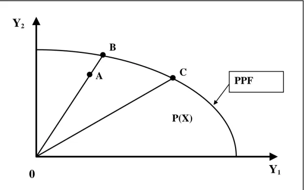
increasing in Y, and decreasing in X, and defined as the maximum feasible expansion of the output vector given the input vector (Cuesta and Orea 2002). Figure 1 illustrates the

concept of an output distance function with two outputs and a given input vector, X. The production possibility set is the area bounded by the production possibility frontier (PPF), which indicates the maximum feasible output given X, and the Y1 and Y2 axes. If the

output vector, Y, is an element of the feasible production set, P(X), Do(X,Y)≤1. For firms

such as B and C in Figure 1 which produce on the PPF, D0(X,Y) =ϖ =1, thereby

indicating technical efficiency. In contrast, for a firm operating at A, D0(X,Y)

=

OB OA

=

ϖ <1, thereby indicating the proportion by which output is below potential output.

Insert Figure 1 about here

This also illustrates that Farrell (1957)’s output-oriented measure of technical efficiency, defined as the maximum producible radial expansion of the output vector, can be represented as:

Y) (X, D

0

OE lies between one and infinity and increases with inefficiency. If Y is located on the

outer boundary of the production possibility set,OE₀ =1, indicating efficiency. In contrast, if Y is in the interior of the production possibility set, indicating inefficiency.

1 0>

OE

3.2 The econometric specification

Following Fare and Primont (1995) and Cuesta and Orea (2002), but also allowing for exogenous factors, the general form of a stochastic output distance function can be shown as follows:

(

nt nt nt

) ( )

nt

o Y X Z h

D _,, _,, _, , _,

1= β ε 5

where h

( )

ε_n,t =exp

(

u_n,t+v_n,t

)

, Y n,tis a vector of outputs, X n,t is an input vector, Z n,t is an

exogenous factor vector and β is a vector of parameters. Inefficiency is accommodated in the specification of h

()

. as εn,t is a composed error term comprised of which

represents random uncontrollable error that affects the n-th firm at time t, and , which is assumed to be attributable to technical inefficiency.

t n v _, t n u ,

In order to facilitate estimation, the authors follow the standard practice of imposing homogeneity of degree one in outputs on the distance function, which implies that D_o

(

Z,X,πY

)

=πD_o

(

Z,X,Y

)

,π >0. By arbitrarily choosing the M-th output, the authors can then defines

M Y 1 = π and write:

(

)

M o M o Y Y X Z D Y Y X Z D , , _⎟⎟= , , ⎠ ⎞ ⎜⎜ ⎝ ⎛ 6

From Equation 5 and after assuming *

(

_{1, , ,,}, _{2, , , ,,}..., _{1, , ,,}

)

. ,t nt Mnt nt Mnt M nt Mnt

n Y Y Y Y Y Y

Y = ₋ and

rearranging terms yields the general form:

(

nt nt nt

)

(

nt o t n M h Z X Y D y , , , * , , , , , , 1 _{β ε}

⋅

=

)

7 Finally after assuming the standard translog functional form1 to represent the technology, the output distance can be represented as:

t n s t n k K s s k K k t n m M m m t n k K k k o t n M X Y X X Y _{, , , ,} 1 , 1 * , , 1 1 , , 1 , , ln ln 0.5 ln ln ln

∑

∑

∑

∑

= = − = = + + + = −

ϕ

α

β

α

, , *, , 1 1 , 1 * , , * , , 1 1 1 1 ,

ln

ln

ln

ln

5

.

0

M _{knt mnt} m m k K k t n j t n m M m M j j m

Y

Y

∑

∑

X

Y

∑∑

− = = − = − =

+

+

β

θ

X t Y t t t Z

_v

_u

8 t n t n, t n h H h h t n m M m t m t n k K k t k ,, , 1 2 2 1 * , , 1 1 , , , 1 , ln + ln + +0.5 + + + +

∑

∑

∑

= − = =

ξ

λ

λ

ψ

δ

where, Y*m,n,t = Y m,n,t / YM,n,t, k=1,2,..K and s=1,2,..K are indices for inputs; m=1,2,…M

and j=1,2,..M are indices for output; h=1,2,…H is an index for environmental variables, and the Greek letters (except v and u) represent unknown parameters to be estimated.

Standard symmetry is imposed to the second order parameters:

α

_k,s=

α

_s,k and

β

β

m j j m, = ,

in Equation 8. vn,t is assumed to be normally distributed with zero mean and variance, .

u

2 v σ

n,t ≥ 0 is drawn from a one-sided distribution and can be assumed to be drawn from one

of four possible distributions, which are the exponential, half-normal, truncated-normal or the gamma distribution. Similar to some studies, un,t is assumed to follow a normal

distribution with zero mean and variance, (e.g. Berger and Mester 1997; Mertens and Urga 2001; Kasman 2005). Given this assumption, the approach of Jondrow, Lovell,

2 u σ

1 _{In the literature, the translog function is preferred in estimating a parametric distance function because it is}

flexible, easy to calculate and permits the imposition of homogeneity (Fuentes, Grifell-Tatjé, and Perelman 2001).

Materov, and Schmidt (1982) is followed to derive the log likelihood which is expressed

in terms of the two variance parameters, and . The

parameters in the translog function as defined in Equation 8 as well as and

σ

σ

σ

2 2 2 u v+ =

γ

σ

2/

σ

2

σ

2 u v u + = 2

σ

γ

are estimated using maximum likelihood estimation (MLE) techniques.

Following from Equation 5, and given current model assumptions, an estimate of output distance can be derived as Do

(

Yn,t,Xn,t,Zn,t,β

)

=exp(−μ) . Equivalently an estimate of Farrell output oriented efficiency is obtainable as:

) exp( , , , _{, ,} , 1 0 ,

μ

β

⎟_⎠⎞= ⎜ ⎝ ⎛ = t n t n t n X Z Y D OEnt 9

However, as OE_n,t relies on the unobservable inefficiency, un,t,, the authors follow the

approach of Jondrow, et al. (1982) and employ the conditional expectation of un,t given the

observed value of overall composed error term, εn,t which can be expressed as:

(

)

(

)

(

)

⎥⎥ ⎥ ⎦ ⎤ ⎢ ⎢ ⎢ ⎣ ⎡ ⎟⎟ ⎟ ⎠ ⎞ ⎜⎜ ⎜ ⎝ ⎛ + =

−

Φ

−

σ

γε

σ

γε

σ

γε

φ

σ

ε

A t n A t n t n A t n A t n

u

E

, , , , ,

1

10 where,

(

)

2 1 γ σ γ

σA = − , φ(.) is the standard normal density function and (.) is the standard normal cumulative distribution function.

Φ

With SFA, it is effectively assumed that firms operate with the same production technology. It is therefore necessary to control for differences in characteristics and the operating environment that may influence the efficient level of output. Failure to account for differences between bank groups may yield inappropriate conclusions about a bank’s performance (Bos and Kool 2006; Bos, Koetter, Kolari, and Kool 2008). Environmental variables are therefore often included directly in the estimated distance function to control for these differences. However, the resulting efficiency scores must be carefully interpreted as estimates of net efficiency after accounting for the impact of environmental influences on potential output. Therefore, OE_n,t provides estimates of efficiency net of

the impact of the environmental Z factors on efficient output. Stated differently, estimates efficiency after allowing for differences in potential output that can be attributed to differences in the included environmental variables, and should therefore be interpreted as a net efficiency estimate (Coelli, et al. 1999).

t n

OE _,

As far as the authors are aware of, no previous output distance function studies in the banking literature have included environmental variables, but a number of cost function studies have included regressors such as bank location and branch banking limitations (Berger and DeYoung 1997), the number of branches, and merger controls (Lozano-Vivas 1998). Although this approach is quite common in the literature, the authors would argue that its suitability is dependent on the assumption that the included environmental variables are factors which only directly influence the production technology, and hence potential output. On the other hand, if some or all of the included environmental factors have a more direct influence on firm efficiency, net efficiency ( ) will give a biased measure of managerial efficiency, because it nets out the impact of such characteristics. This therefore implies that the common exercise of reporting efficiency scores after including factors such private or foreign ownership directly in the function is likely to result in biased measures of efficiency if these factors are associated more with differences in efficiency rather than differences in production technology.

t n

OE _,

As the current study includes several Z factors, such as foreign ownership and a dummy for Islamic banks, which could be argued to have a greater direct influence on inefficiency rather than the location of the efficient frontier, the authors will investigate the potential implications of this on the efficiency scores. The approach of Coelli, et al (1999) is therefore employed to generate alternative gross efficiency

(

GE_n,t

)

estimates.

In order to do this, the authors first identify the observation with the most favorable operating characteristics given the estimated parameters. This observation will have the minimum value of , which will be referred to as . If it is assumed that other firms face this most favoured operating environment, rather than their own, the authors can estimate a predicted efficient output for firms under the assumption that all firms face this most favoured operating environment.

⎥ ⎦ ⎤ ⎢ ⎣ ⎡

∑

= H h t n h h

Z

1

ξ

,, ⎥⎦ ⎤ ⎢ ⎣ ⎡

∑

= H h t n h h

Z

Min 1

ξ

,,

As the observation used for this purpose, is the observation with the most extreme observed value, it functions as a benchmark for the hypothetical firm that benefits from the most favorable environmental conditions. This is because the firm with , faces the most favorable operating environment

basedon the model’s parameters, and this is regardless of the sign of the ⎥ ⎦ ⎤ ⎢ ⎣ ⎡

∑

= H h t n h h

Z

Min 1

ξ

, , ⎥ ⎦ ⎤ ⎢ ⎣ ⎡

∑

= H h 1

ξ

h

Z

h,n,t ⎥ ⎦ ⎤ ⎢ ⎣ ⎡

∑

= H h t n h h

Z

Min 1

ξ

, ,

ξ

parameter. This generates an adjusted estimate of the deviation of a firm’s actual output from frontier output, which can be expressed as:

_⎥ 11 ⎦ ⎤ ⎢ ⎣ ⎡ − + =

∑

∑

= = H h t n h h H h t n h h t n Gross t n

Z

Min

Z

1 , , 1 , , , ,

ε

ξ

ξ

ε

Measures of the firm’s gross inefficiency can then be derived by substituting for in Equation 10, yielding:

Gross t n, μ Gross t n,

ε

t n, ε _, exp( Gross_, ) 12 t n t n GE =

μ

Because

(

GE_n,t

)

is computed under the assumption that a firm faces the most favourable

operating environment, differences in operating environment as well as differences in net efficiency will be reflected as differences in . This is not the case with , which by definition nets out the impact of differences in operating environment (Coelli, et al. 1999). It would be inappropriate to assess relative managerial performance with if all the exogenous factors only influenced the production technology. Nevertheless, if it can be argued that some or all of these factors have an influence on expected managerial efficiency, will better attribute differences in measured efficiency to differences in these factors. t n GE _, OE_n,t t n GE _, t n GE _,

Given the estimated model, estimated scale elasticity can be calculated as the negative of the sum of the input elasticities (Cuesta and Orea 2002):

(

)

∑

= ∂ ∂ − = K k knt t n k t n m o t n X X Y D SCALE 1 , , , , , , , ln , ln 13

If , a bank is operating with increasing returns to scale (IRS). If , there is decreasing returns to scale (DRS) and constant returns to scale (CRS) are present if 1 ,t > n SCALE 1 ,t < n SCALE 1 ,t = n SCALE .

Malmquist productivity indices are commonly used in the literature because they require neither price information nor restrictive behavioural assumptions such as cost minimization or profit maximization. Moreover, they can be readily employed to isolate efficiency change from technical change (Färe, Grosskopf, Norris, and Zhang 1994; Grifell-Tatje and Lovell 1995; Isik and Hassan 2003). However, as Caves, Christensen, and Diewert (1982) prove, the parametric Mamquist index will give a biased estimate of TFPC, that excludes the impact of scale changes, unless firms operate with CRS. Orea’s (2002) generalised Malmquist Productivity Index provides a solution to this issue by adding a scale term (which, vanishes under CRS) to the Malmquist Productivity Index, thus providing a theoretically unbiased measure of TFPC. Therefore, Orea (2002)’s approach extends the standard Malmquist Productivity Index which captures only the impact of technical efficiency change (TEC) and technical change (TC), by further allowing for the impact of scale change effects (SCE) on productivity change. The authors therefore employ previously estimated output distance function and inefficiency estimates to calculate TFPC and decompose it such that, TFPC =TEC +TC +SCE .

Thus, for any given periods t and t+1, a generalised output-oriented Malmquist Productivity Index can be expressed as:

TFPC =ln

(

TFP_n,t+1 TFP_n,t

)

= ln

(

D0,_n,_t+1 D0,_n,_t

)

−0.5

[

(

∂ln D0,_n,_t+1 ∂t

) (

+ ∂lnD0,_n,_t ∂t

)

]

[

(

)

(

)

]

⎟ ⎟ ⎠ ⎞ ⎜ ⎜ ⎝ ⎛ Ω − + ∑ = − Ω + + + + t n k t n k t n t n OM t n t n OM X X SCALE K k SCALE , , 1 , , , , , 1 , 1 , , 1 .ln 1 1 5 . 0 14 where; t n OM k t n t n SCALE X D , , , . 0 , ln ∂ ∂ − = Ω

The first term on the right hand side of Equation 14 is TEC, which measures the contribution of efficiency change to productivity. The second term is TC, which measure the contribution of technical change. The final term is SCE, which measures the contribution of changes in scale to productivity change. With IRS (DRS), increases in scale result in increased (decreased) productivity, while under CRS, this final term, SCE vanishes and TFPC is equivalent to a standard Malmquist Productivity Index.

3.3 The data and empirical specifications

Similar to Cuesta and Orea (2002), the intermediation approach is employed to define bank output, as it is the most suitable with the concept of Islamic banking. The selection of the input and output variables follows the existing literature (e.g., Iqbal, et al. 1999; Cuesta and Orea 2002; Cuesta and Zofío 2005). The outputs are loans (Y1) and total

other earning assets (Y2), and the inputs are labour (X1), deposits (X2), and capital (fixed

assets) (X3). X1is the number of full time workers, X2 is total deposits including customer

funding and short term funding, and X3 is the total expenses on fixed assets allocated for

all furniture, equipment, and bank premises, including depreciation, and administration and general expenses. It is noted that linear homogeneity in outputs is imposed using Y2

as a numeraire and these variables have been mean-corrected prior to estimation. Table 1 provides a summary of descriptive statistics of these variables and the explanatory variables for all banks in the sample. All monetary variables are expressed in MYR and in real 2000 terms by deflating with the Malaysian GDP deflator index.

The first operating environment variable is loan quality (Z1), as proxied by the

ratio of the NPLs-to-total loans (e.g., Clark 1996; Mester 1996; Berger and Mester 1997; Girardone, Molyneux, and Gardener 2004; Williams and Nguyen 2005). If output quality is not controlled for, unmeasured differences in loan quality that are not captured by banking data may be mistakenly measured as inefficiency (Berger and Mester 1997). This is because banks with better loan quality may appear inefficient as they use more labour and capital to monitor loans (Mester 1996). Moreover, as the East Asian financial crisis caused banks’ NPL to rise during the sample period, this negative economic shock would have caused some banks extra expenses to recover defaulted loans and related administration costs (Berger and DeYoung 1997). Therefore, a positive coefficient is expected for this quality variable, indicating that banks with higher NPL-to-loans (lower loan quality) produce lower output.

The rest of the environmental variables are dummy variables that are designed to capture potential differences in bank characteristics and operating environment that may influence bank output. These environmental variables may capture either legitimate output changes or inefficiency, depending on the assumption with regard to whether these variables directly influence the production technology or more directly influence firm efficiency. Thus, the dummy variable indicating full-fledged Islamic banks (Z2) is to

control for the potential impact of full-fledged Islamic banking on bank output. No a

priori assumption is made due to mixed results in the literature on the direction of these

effects (e.g., Al-Jarrah and Molyneux 2005; El-Gamal and Inanoglu 2005; Mokhtar, Abdullah, and Al-Habshi 2006).

The model also includes a dummy variable for foreign banks (Z3), foreign banks

with IBS (Z4) and all banks with IBS (Z9), leaving conventional domestic banks without

IBS as the base case measured in the constant, where banks with IBS are conventional banks offering Islamic banking products through a separate Islamic banking window. When predicting the expected impact of these dummy variables on efficient output, it is noted that relative to domestic banks, foreign banks have better access to multinational clients and priority access to technology from their parent banks (Berger, Clarke, Cull, Klapper, and Udell 2005). Moreover, in the literature, foreign owned banks are found to be more efficient relative to domestic banks in Malaysia (Matthews and Ismail 2006; Mokhtar, et al. 2006) and other countries (Bhattacharyya, Lovell, and Sahay 1997; Sturm

and Williams 2004; Bonin, Hasan, and Wachtel 2005; Berger, Hasan, and Zhou 2008) but not in the USA (Mahajan, Rangan, and Zardkoohi 1996; Chang, Hasan, and Hunter 1998). Hence, the foreign-owned dummy (Z3) is expected to have a negative coefficient

indicating higher potential output.

Considering banks operating IBS windows, there is a less straight forward expected relationship. The provision of IBS windows may increase efficient output by allowing a bank to tap additional market segments with its existing workers and facilities. However, higher input requirements may be associated with Islamic financing and/ or the need to maintain strict financial separation between Islamic and non-Islamic operations. Therefore, the uncertainty with regard to the likely impact of IBS banking services on efficient output implies that the authors cannot a priori predict the sign of the coefficients

for the Z4 and Z9 variables.

Insert Table 1 about here

A dummy variable for observations in 1998 is included to control for the East Asian financial crisis (Z5). The financial crisis started to affect the Malaysian banking

sector in the third quarter of 1997 when a small decline in credit expansion occurred. However, previous good macroeconomic performance and the persistence pace of credit expansion before the crisis contributed to overall bank loan growth that remained strong in 1998. In reaction to the financial crisis, banks reduced a large number of employees and reduced other expenses drastically at the end of 1997 and throughout 1998 (Central Bank of Malaysia 1997, 1998, 1999). Interest rates, which were initially increased at the end of 1997 and in the first half of 1998 to support MYR exchange rates in order to discourage capital outflows, were subsequently reduced in the third quarter of 1998 to support the economic recovery plan. Other government actions to support consistent bank loan growth included a government general guarantee of deposits, a reduction of reserve requirements, several prudential measures such as accelerating non-performing, doubtful and bad loans classifications, frequent and detailed reports on NPLs, and intensified central bank monitoring of banks. Furthermore, the government established a public company (Danaharta) for purchasing NPLs from banking institutions to ensure that the

institutions in managing the NPLs, and established a central bank owned company

(Danamodal) to inject new capital in undercapitalized banks. Selected NPLs were

restructured by the Corporate Debt Restructuring Committee (CDRC), which then exempted them from NPL classification. The CDRC was a facilitator in bringing creditors and debtors to the negotiating table and in sorting out an agreeable and workable loan restructuring exercise as an alternative option to companies filing for bankruptcy. Some cases had been transferred to Danaharta (Lindgren, Balino, Enoch, Gulde, Quintyn, and

Teo 1999; Ariff, Setapa, and Lin 2001). As a result of these actions, much of the effect of the financial crisis was concentrated in 1998 as demonstrated by Malaysian GDP growth, which was respectively 7.3, -7.4, and 6.1 percent in 1997, 1998 and 1999 (Ministry of Finance Malaysia 1999). Given that overall bank loan growth remained strong in 1998, it is expected that the relationship of raised output and the financial crisis (Z5) to occur in

1998 when banks duality reduction in the operating inputs and deposits take place.2 _The

reduction in the operating inputs is a result of the elimination of a large number of workers as well as cutting other expenses, and the drop in the deposits is due to a decline in interest rates.

Finally, given that some banks have gone through mergers, one can control for this effect by using a merger dummy variable (Z10). However, as it is found that this dummy

for all merged banks is not statistically significant, the authors also test for the potential effects of individual mergers, finding that the dummy is significant for 3 individual mergers, merger 1 (Z6), merger 2 (Z7) and merger 3 (Z8).3 These dummy variables are

expected to have a positive coefficient indicating lower output because merged banks need some time for system integration and personnel integration (Peristani 1997; Rhoades 1998; Sherman and Rupert 2006).

2 _{Dummy variables for 1996, 1997, all post-crisis years, as well as individual dummy variables for each of}

the years after 1998 were tested but were found to be statistically insignificant. It is noted that the increase

in bad loans that was associated with the crisis are controlled for with the Z1 variable. 3 _{Merger 1, 2, 3 refer to mergers between Oriental Bank and EON Bank, between Chung Khiaw Bank and}

4 RESULTS

4.1 The output distance function estimates

The estimated output distance function parameters are reported in Table 2. All models have the same inputs and outputs but different environmental variables. Model A includes the first nine environmental variables (Z1-Z9), described earlier, while Model B

excludes the banks with IBS (Z9) dummy variable, which is insignificant in Model A. As

the log likelihood ratio test for the inclusion of (Z9) is 0.02, the null hypothesis that this

parameter is insignificant cannot be rejected, and as it is preferred, the following discussion will be limited to Model B. However, it is noted that as conventional domestic banks without IBS windows are the base case in Model A, this result suggest that, ceteris

paribus, no statistically significant difference in efficient output can be identified for the

group made up of conventional domestic banks with IBS and domestic banks without IBS. Finally, Model C is included solely to illustrate the statistical insignificance of the aggregate merger dummy (Z10). This finding is consistent with Berger and Humphrey

(1997), which noted that some mergers improve cost efficiency whereas others worsen it. Recalling that , the highly significant estimate of 0.826 for this parameter suggests that the portion of technical inefficiency in total variance is high. Thus, the estimated deviation from the frontier is mainly due to inefficiency rather than statistical noise. The estimated coefficients of all variables have the expected signs. Loan quality

(ζ

σ

σ

σ

γ

2 2 2 / u v u + =

1) is positive as predicted, and indicates that lower output quality (higher NPL-to-loan

ratio) reduces output, thereby reflecting the higher input requirement needed to monitor default loans.

Moreover, as the NPL-to-loan ratio increases significantly from 6 to 17 percent for the average bank between 1997-1999, the results suggest that outputs decrease by 4.3 percent on the efficient frontier for the hypothetical average bank because of the effects of the East Asian financial crisis on bad loans. Furthermore, as the NPL-to-loan ratio remained stable at approximately 16 percent after 1999, this decline in output that could be due to the impact of financial crisis on non-performing loans is still relevant until the end of the sample period.

The positive estimate for ζ2 implies that full-fledged Islamic banks are found to

have outputs that ceteris paribus are 6.6 percent lower than other banks and this may be

banking. The coefficient for foreign-owned banks is negative, indicating that output increases by 14.0 percent relative to domestic banks. However, foreign-owned banks with IBS (Z4) are found to have potential output that is 11.8 percent lower than foreign banks

without IBS. The coefficient for the financial crisis dummy variable (Z5) is negative,

indicating that output increased by 2.7 percent in 1998 after controlling for other variables. This finding is consistent with the reactions of banks towards the financial crisis, which was to lay off substantial number of workers and to cut other operating expenses. The individual mergers (Z6, Z7, Z8) are found to be associated with output that is 8.3 percent,

9.7 percent and 6.3 percent lower respectively, after controlling for other variables.

Insert Table 2 about here

4.2 Net and Gross Efficiency Estimates

Table 3 and 4 respectively provide estimated net and gross efficiency for Model B. As expected, given earlier theoretical discussion, average net efficiency is higher than average gross efficiency. Thus, net efficiency of Malaysian commercial banks is on average 1.055, and ranges from 1.011 to 1.220, hence on average, banks only produce 94.8 percent4 of the output they could produce if they operated on the efficient frontier. In contrast, average gross efficiency is 1.215, thus signifying that the outputs of the average bank are only 82.3 percent5 of what they could be if they operated on the frontier defined by the most favourable operating environment. In addition, the gross efficiency estimates range from 1.014 to 1.445. Hence, while the net efficiency scores demonstrate that while there is comparatively little variation in estimated efficiency once differences in the environmental variables are controlled for, the gross efficiency scores suggest that substantial differences in outputs can in fact be attributed to differences in operating environment.

Table 3 and 4 also demonstrate that the yearly average and the range of the efficiency scores, has risen for both net and gross efficiency. The trends in net efficiency imply a deteriorating in average efficiency over the sample period, but also the existence of a group of banks that were steadily deviating from the output frontier. Hence, average

4 _{OE=(1/ 1.055)100} 5 _{GE=(1/ 1.215)100}

net efficiency worsened from 1.042 in 1996 to 1.060 in 2002 and the maximum net efficiency score deteriorated from 1.104 in 1996 to 1.211 in 2002.

Table 3 also shows that after netting out the impact of environmental factors, the efficiency estimates of different bank categories unfailingly cluster around the overall mean, with a minimum group average of 1.04 for merged banks with IBS and a maximum group average of 1.062 for foreign banks without IBS. Hence, once the impact of operating characteristics on estimated outputs is netted out, there is little further difference in estimated efficiency across the identified categories. In other words, if efficiency is judged against an efficient frontier, which for example, allows full-fledged Islamic banks to have 6.6 percent lower output and requires foreign banks without IBS to have 14 percent higher outputs, it should be expected that the resulting net efficiency scores exhibit small difference across these groups.

Insert Table 3 about here

On the contrary, because the gross efficiency estimates reported in Table 4 incorporate the impact of net efficiency as well that of unfavourable operating characteristics, they produce substantial information related to the main determinant of variation in the input requirements of banks across the various identified categories. Furthermore, these differences are largely consistent with the preceding explanation of the output impacts for the related dummy variables in Table 2. Hence, while the average gross efficiency score is 1.215 for all banks, foreign banks have average gross efficiency of 1.161, indicating relatively higher outputs for these banks. Likewise, the poorer average gross efficiency estimates for merged banks (1.238) versus unmerged banks (1.210) imply that the merger activities in Malaysian banking may have played a part in reducing bank outputs.

Insert Table 4 about here

Concentrating on Islamic banking, full-fledged Islamic banks have average gross efficiency equal to 1.311, hence clearly suggesting that full-fledged Islamic banking can be linked with higher input requirements. Furthermore, the group of all conventional banks without IBS have average gross efficiency of 1.152, while those with Islamic

banking windows have higher input requirements as demonstrated by deteriorating gross efficiency (1.236).6 Thus, after the influence of operating characteristics on input requirements is allowed for, these findings suggest an obvious order with pure conventional banks showing the best output performance, followed by conventional banks that operate IBS windows, and finally full-fledged Islamic banks with the worst output performance.

Focussing on the impact of the East Asian financial crisis, there is a similarity in the net and gross efficiency estimates as they respectively deteriorated from 1.042 and 1.163 in 1996 to 1.061 and 1.207 in 1997. Moreover, this deterioration in average estimated efficiency is observed across categories. Nonetheless, efficiencies improved in 1998. This demonstrates that despite current findings that there was not a statistically significant impact of the financial crisis in 1997 as identified by a dummy variable for that year, the net and gross efficiency estimates suggest there may still been a detrimental impact in 1997.7

Lastly, focussing on the general trend in gross efficiency, the average estimates demonstrate that average gross efficiency improved marginally from 1.207 in 1997 to 1.200 in 1998, and this improvement in average estimated gross efficiency is noted across all categories. Nevertheless, average gross efficiency rose to 1.235 in 1999 and remained close to this level until 2002. Hence, the findings suggest a transitory improvement in general output performance in 1998 followed by a sustained decline in output performance. These results can be interpreted as manifesting the double impact of the financial crisis on output efficiency. Thus, the prolonged deterioration in gross efficiency after 1998 reflects the sustained increase in NPLs and the resulting increase in input requirements discussed earlier. On the contrary, the interim improvement in gross efficiency in 1998 reflects an immediate but temporary reaction to the financial crisis which can be attributed to a decrease in input usage as a result of the elimination of a large

6 _{It s noted that higher input requirements as reflected by higher average gross efficiency estimates for IBS}

banks are also observed within the domestic banks, foreign banks, merged banks and unmerged banks categories, thereby supporting this conclusion. However, the difference is marginal within the domestic bank category, consistent with the finding regarding the statistical insignificance of the Z9 variable. 7 _{High interest rates at the end of 1997 as the Malaysian government tried to reduce capital outflows,}

contributed to a decline in credit growth from an annual average of 30 percent to 26.5 percent at the end of 1997 (Lindgren, et al. 1999). Given the relative small size of this effect, this may explain for insignificant year 1997 dummy when tested in the model.

number of workers, cuts in other operating expenses, and declines in interest rates.8 On the other hand, in the long run, it is obvious that deterioration in loan quality, which can be attributed to the financial crisis, has had a considerable negative impact on potential output in the Malaysian banking sector.

4.3 Returns to Scale

Table 5 shows firm specific return to scale estimates for all banks and by bank category. The average estimated return to scale is 0.990, thereby indicating the presence of mild decreasing return to scale. The range of estimated returns to scale is between 0.856 and 1.092, and is consistent with the previous output-oriented literature (e.g., Cuesta and Orea 2002).

On average, this estimated scale elasticity has decreased from 1.018 in 1996 to 0.967 in 2002, and this finding is consistent with the overall increase in the scale of banks through mergers discussed above. Likewise, within almost all bank categories summarised in Table 5, very mild decreasing returns to scale and a slight downward trend in estimates is observed. Thus, there is little evidence for a difference in returns to scale across the groups identified in Table 5.9 The existence of mild increasing return to scale in 1996, the slight decreasing return to scale towards the end of the sample period and the consolidation of banks, suggests that if total factor productivity change in Malaysian banking was affected by scale change effects during 1996-2002, this effect is likely to be only a slight decrease on average.

Insert Table 5 about here

4.4 Productivity Change and its Decomposition

Table 6 gives average estimated productivity change across all banks and its decomposition into efficiency change, technical change and scale change. Over the sample period, average productivity change was 2.37 percent per year. As technical change increased 2.79 percent, productivity change is largely driven by technical

8 _{Interest rates, which were very high to refrain capital outflow, were reduced in the third quarter of 1998 to}

support the economic recovery plan.

9 _{Yudistira (2004) found that small and medium-sized Islamic banks in most countries have diseconomies of}

change.10 However, as estimated average technical change declined from 3.95 percent in 1997 to 1.72 percent in 2002, the trend decrease in overall productivity change can also be attributed to decreasing rates of technical change.

The negative average scale change effect of 0.03 is consistent with the result of average mild decreasing returns to scale, but also strengthens the finding that mergers have not contributed to productivity increases. Between 1996 and 1997, scale change contributed a 0.28 percent increase in productivity change, but this cannot be attributed to mergers, which only occurred later in the sample period. The succeeding year saw a negative scale change effect of 0.18 percent, which possibly signals deterioration in output due to the financial crisis and reduced economic growth in 1998.

Insert Table 6 about here

While technical change has influenced the long term descending trend in average productivity change, efficiency change has been accountable for dramatic variations around this trend. The pattern of annual efficiency is quite unpredictable, with big positive contributions to productivity change in 1998 and 2001, but large negative effects in other years. While, efficiency change reduced average productivity change by 2.24 percent in 1997, efficiency change contributed 0.6 percent to productivity change in 1998 before dropping again in the subsequent years. Overall, the results suggest that the financial crisis adversely affected productivity. This decline in productivity was caused by a decline in net and gross efficiency in 1997 which can be attributed to the financial crisis. Moreover, the gross efficiency estimates indicate that the financial crisis has had a continued output reducing impact by triggering a sustained increase in NPLs.

4.5 Firm specific productivity change and its decomposition

Table 7 shows productivity change estimates over the sample period for all banks and by bank category. It also decomposes these rates into efficiency change, technical

10 _{This result is similar to findings by Orea (2002) on Spanish banks, Isik and Hassan (2003) for Turkish}

banks and Casu, Girardone, and Molyneux (2004) on Spanish and Italian banks where technological progress is the main determinant of productivity change. Krishnasamy, et al. (2004) found productivity

improvement in 10 Malaysian commercial banks was also primarily determined by technical change during the 2000-2001 period.

change, and the scale change effect. It is clear that considerable differences exist between average productivity change for various bank categories. Thus, the small group of merged banks without IBS have the highest average productivity change at 3.33 percent, while the minimum group average of 0.54 is for merged banks with IBS. The latter group contributes to the lower average productivity change in merged banks (1.57 percent), relative to unmerged banks (2.50 percent).11 Compared to all domestic banks (2.19 percent), foreign banks have higher average productivity change (2.68 percent), but this can be primarily attributed to the foreign banks without IBS group (3.10 percent).

The decomposition of productivity change gives some important insights into these considerable differences in productivity change across bank categories. The much lower average productivity change of 1.57 percent for unmerged banks relative to merged banks can be mainly attributed to higher rates of technical change for the unmerged banks (2.93 percent) compared to the merged banks (1.88 percent), perhaps because merged banks need to concentrate more on integrating staff and coordinating their systems (Rhoades 1998; Sherman and Rupert 2006).12

Insert Table 7 about here

However, the identical 0.03 percent deterioration in average productivity change attributed to scale change effects for both merged and unmerged banks suggests that mergers have not contributed to productivity change through scale effects.

Much of the difference in productivity change between merged and unmerged banks can be attributed to the 0.54 average productivity change for merged banks with IBS windows, which can mainly be attributed to very low technical change (1.64 percent) and a considerable decline in efficiency (-1.10 percent). When coupled with the relatively small difference in estimated productivity change, technical change, efficiency change, and scale change effects for unmerged banks with or without IBS windows, this demonstrates a further disturbing impact of Malaysian banking mergers during the chosen

11 _{Sufian and Ibrahim (2005) reported average total productivity growth for post-merger Malaysian banks of}

-1.3 percent for the period 2001-2003.

12

The result is consistent with Orea (2002)’s research who finds that the average rate of productivity change of merging banks is lower than non-merging banks, and Berger and Mester (2003) who found that productivity deterioration is greater for merging banks than non-merging banks.

sample period. This is because it suggests that merged banks with IBS banking windows may have been unable to allocate adequate managerial effect to developing their IBS operations, because their managers were distracted by these mergers.

The comparatively low average productivity change of foreign banks that have IBS windows in operation is attributable to relatively low average technical change (2.22 percent) as well as deterioration in efficiency 0.44) and a negative scale change effect (-0.09). As foreign banks without IBS have comparatively fast technical change (3.05 percent) and positive efficiency change and scale change effects, these results imply that foreign banks that operate IBS have not only failed to develop new technologies, but have also become less efficient over time. This may suggest that although these banks moved into the developing market of Islamic banking services, they were very slow in developing new products and technologies for this market. On the contrary, foreign banks that have continued concentrating on conventional banking services managed to maintain technical change and have been more able to sustain efficiency levels. Therefore, the findings may suggest that, for foreign banks, venturing into the Islamic banking market has been a disruption from their principal proficiency.

The authors finally focus on Islamic banking. Large differences in average productivity, technical change and efficiency change between the group of all conventional banks with or without IBS windows, implies that there is a sizeable difference in productivity change that can be generally attributed to the provision of Islamic banking services by conventional banks. The foregoing discussion proposes that both foreign banks and merged banks that offered IBS banking services have faced lower average rates of productivity change. Similarly, the lower than average productivity change for full-fledged Islamic banks (1.93)13 can be mainly explained by relatively low technical change (2.66 percent), as well as deterioration in efficiency change (-0.44 percent) and a negative scale change effect (-0.29 percent). This suggests that while Islamic banks have been moderately successful in developing new output enhancing products and technologies,14 they have been unable to remove inefficiencies in their operation.

13 _{Moderate productivity growth is found in Islamic banks for most countries (Hassan 2005) but productivity}

loss is found for Islamic banks in Sudan, Iran and Pakistan (Hassan 2003).

14 _{This is consistent with Hassan (2003; 2005) who also found that the productivity change of Islamic banks}

5 CONCLUSIONS AND POLICY IMPLICATIONS

The objective of this paper was to investigate the efficiency, economies of scale and productivity of Islamic banks relative to conventional banks using an output distance function and a generalised parametric Malmquist Productivity Index. In achieving this goal, some significant results with regard to the Malaysian banking sector are found. The average Malaysian bank is estimated to produce only 94.8 percent of the output that could be produced if it operated on the frontier defined by actual operating characteristics, but only produces 82.3 percent of the potential output that could be produced if it instead faced the most favourable operating environment. This suggests that differences in bank characteristics play an important role in determining bank outputs. Moreover, on average, banks became more inefficient between 1996 and 2002, causing an average 0.39 percent decline in productivity change. The finding that banks operate at or near to constant returns to scale is also consistent with the finding that scale change contributed only a 0.03 percent decrease in average productivity change. As technical change contributed 2.79 percent to average productivity change, it was the main determinant of productivity change which averaged 2.37 percent per year between 1996 and 2002.

The estimates of gross efficiency allow better understanding of the determinants of variation in outputs across bank categories, because, by definition, net efficiency estimates net out the influence of operating characteristics on bank output by first allowing for increases or decreases in predicted efficient output attributable to the operating environment. In contrast, the gross efficiency estimates are measured relative to an efficient frontier with the most favourable observed operating environment as gross efficiency implicitly includes not only the impact of net inefficiency but also the impact of decreased outputs associated with an unfavourable operating environment. Hence, gross efficiency highlights the impact of all operating characteristics on bank outputs. Therefore, regardless of whether one believes that operating characteristics should directly influence inefficiency (gross efficiency) or one believes that they influence the efficient output frontier (net efficiency), the gross efficiency estimates provided in this paper has increased the authors’ understanding of the effect of differences in operating characteristics on observed differences in bank outputs. As a result, the finding of slight

differences in net efficiency, imply that it is the differences in operating characteristics which explain a large amount of the output differences between Malaysian banks. Thus, for example, the high gross efficiency estimates for both full-fledged Islamic banks and conventional banks with IBS windows imply that Islamic banking requires considerably higher inputs, a finding that is not revealed in the net efficiency estimates. Likewise, while net efficiency demonstrates little effect from the East Asian financial crisis, the gross efficiency estimates clearly demonstrate that the crisis had an interim output increasing effect in 1998. Moreover, the gross efficiency estimates subsequently demonstrated that the crisis prompted a continuing negative impact on the output performance of Malaysian banks, which can be attributed to an increase in non-performing loans.

Given the extensive bank mergers in Malaysia during the chosen sample period, it is also remarkable that merged banks have experienced substantially lower productivity change relative to unmerged banks. However, this difference can be mainly attributed to the lower efficiency change of merged banks that operate IBS windows. This implies that the call for managers to simultaneously develop new Islamic banking products and consolidate operations after mergers, may have contributed to this bad performance. However, it also suggests that, in general, mergers do not positively influence the performance of Malaysian banks.

In sum, current output distance function results suggest that the potential for Islamic banks to overcome the output disadvantages associated with Islamic banking are relatively limited. Given the moderate growth of Islamic banking, the existing output disadvantages highlighted by the gross efficiency estimates, and the relatively small output productivity change of Islamic banks when compared to other banks, policy makers in Malaysia face an interesting conundrum. Thus, if they wish to further develop Islamic banking, current results suggest that they will need to better motivate Islamic bank managers to reduce these output disadvantages, and more significantly, they will need to actively work to create a more encouraging banking environment for Islamic banking.

Table 1

Descriptive statistics for sample banks, 1996-2002a

Symbol Variables Mean Std. Dev Minimum Maximum

Outputs

Y1 Loans (MYR, million) 103.85 130.21 1.46 767.7

Y2 Other Earning Assets (MYR, million) 56.76 71.04 1.52 357.56

Inputs

X1 Labour 2,514.27 3,041.24 69.00 20,312.00

X2 Deposits (MYR, million) 143.82 176.27 4.79 977.07

X3 Capital (MYR, million) 1.04 1.20 0.02 6.49

Control Variables

Z1 Loan Quality 0.13 0.12 0.01 0.77

Z2 Islamic bank dummy 0.06 0.24 0 1

Z3 Foreign owned Bank dummy 0.37 0.48 0 1

Z4 Foreign with IBS dummy 0.11 0.32 0 1

Z5 Financial Crisis Dummy 0.17 0.37 0 1

Z6 Merged Bank 1 Dummy 0.01 0.11 0 1

Z7 Merged Bank 2 Dummy 0.04 0.19 0 1

Z8 Merged Bank 3 Dummy 0.01 0.11 0 1

Z9 Banks with IBS Dummy 0.64 0.48 0 1

Table 2

Maximum likelihood estimates for parameters of the output distance function for Malaysian banks: 1996-2002

Parameters Coefficient Model A Model B Model C

Estimated Value Std Error Estimated Value Std Error Estimated Value Std Error φ0 Constant -0.099*** 0.032 -0.104*** 0.014 -0.102*** 0.018 α1 ln X1 -0.039 0.024 -0.039* 0.024 -0.038 0.025 α2 ln X2 -0.914*** 0.022 -0.913*** 0.022 -0.905*** 0.023 α3 ln X3 -0.034** 0.016 -0.034** 0.017 -0.043** 0.017 α1,1 (ln X1)2 0.110* 0.060 0.111* 0.060 0.122** 0.059 α2,2 (ln X2)2 0.038 0.056 0.041 0.053 0.070 0.054 α3,3 (ln X3)2 0.090** 0.037 0.090** 0.037 0.087** 0.040 α1,2 ln X1 ln X2 -0.069 0.046 -0.072* 0.043 -0.101** 0.041 α1,3 ln X1 ln X3 -0.057* 0.032 -0.056* 0.032 -0.057* 0.034 α2,3 ln X2 ln X3 0.012 0.042 0.013 0.043 0.018 0.044 β1 ln Y1 0.596*** 0.012 0.596*** 0.012 0.593*** 0.012 β1,1 (ln Y1)2 0.223*** 0.017 0.223*** 0.018 0.211*** 0.018 θ1,1 ln X1 ln Y1 0.003 0.027 0.003 0.027 0.004 0.027 θ2,1 ln X2 ln Y1 -0.008 0.037 -0.008 0.036 -0.001 0.037 θ3,1 ln X3 ln Y1 -0.035* 0.021 -0.036* 0.022 -0.035 0.023 λ1 t -0.026*** 0.003 -0.026*** 0.003 -0.026*** 0.004 λ11 t2 0.004 0.003 0.004 0.003 0.004 0.003 δ1 ln X1t -0.001 0.008 -0.001 0.008 -0.004 0.008 δ2 ln X2t 0.001 0.010 0.001 0.010 0.002 0.010 δ3 ln X3t 0.004 0.007 0.004 0.007 0.005 0.007 ψ1 ln Y1 t -0.004 0.005 -0.004 0.005 -0.002 0.005 ζ1 _{Loan Quality 0.380*** 0.048 0.380*** 0.048 0.391*** 0.048} ζ2 _{Islamic Bank 0.061* 0.033 0.066*** 0.021 0.058*** 0.022}

ζ3 Foreign Owned Bank -0.146*** 0.040 -0.140*** 0.027 -0.095*** 0.020

ζ4 Foreign with IBS 0.124*** 0.045 0.118*** 0.031 0.070*** 0.026

ζ5 Financial Crisis -0.027** 0.012 -0.027*** 0.012 -0.024*** 0.012

ζ6 Merged Bank 1 0.083*** 0.035 0.083*** 0.035

ζ7 _{Merged Bank 2 0.098*** 0.034 0.097*** 0.034}

ζ8 _{Merged Bank 3 0.063* 0.038 0.063* 0.038}

ζ9 Banks with IBS -0.005 0.029

ζ10 Merged Banks 0.017 0.018

σ2 Sigma-squared 0.005 0.001 0.005 0.001 0.005 0.002

Γ Gamma 0.828*** 0.150 0.826*** 0.143 0.783 0.193

Log Likelihood 268.16 268.14 261.80

Notes:

*,**,*** Significant at 90, 95 and 99 percent confidence level.

α

Table 3

Net efficiency for all banks and by category

1996 1997 1998 1999 2000 2001 2002 All Years

Descriptive Statistics: All Banks

Average 1.042 1.061 1.054 1.052 1.060 1.050 1.060 1.055

Standard Deviation 0.023 0.027 0.034 0.026 0.052 0.037 0.044 0.036

Minimum 1.016 1.015 1.014 1.015 1.011 1.015 1.015 1.011

Maximum 1.104 1.109 1.161 1.123 1.220 1.144 1.211 1.220

Average Efficiency by Category

All Banks 1.042 1.061 1.054 1.052 1.060 1.050 1.060 1.055 Without IBS 1.043 1.062 1.056 1.055 1.069 1.063 1.069 1.060 With IBS 1.041 1.060 1.055 1.052 1.054 1.041 1.052 1.052 Islamic 1.037 1.066 1.017 1.028 1.061 1.062 1.086 1.057 Foreign 1.057 1.068 1.053 1.049 1.061 1.052 1.071 1.059 Without IBS 1.052 1.065 1.060 1.053 1.067 1.057 1.074 1.062 With IBS 1.078 1.077 1.031 1.040 1.043 1.043 1.066 1.052 Domestic 1.035 1.058 1.054 1.053 1.060 1.049 1.051 1.052 Without IBS 1.027 1.046 1.028 1.064 1.080 1.105 1.036 1.052 With IBS 1.037 1.058 1.057 1.054 1.058 1.040 1.046 1.052 Islamic 1.037 1.066 1.017 1.028 1.061 1.062 1.086 1.057 Merged Banksab - 1.077 1.037 1.043 1.044 1.039 1.046 1.044 Without IBS - 1.077 1.037 1.034 1.060 1.068 1.037 1.053 With IBS - - - 1.048 1.028 1.032 1.048 1.040 Unmerged Banks 1.042 1.060 1.054 1.053 1.063 1.058 1.071 1.057 Without IBS 1.043 1.060 1.053 1.054 1.069 1.061 1.081 1.061 With IBS 1.041 1.060 1.055 1.052 1.059 1.053 1.057 1.055 Notes:

a _{No mergers between Islamic banks have occurred during the sample period.} b _{Includes 2 foreign mergers.}

Table 4

Gross efficiency for all banks and by category

1996 1997 1998 1999 2000 2001 2002 All Years

Descriptive Statistics: All Banks

Average 1.163 1.207 1.200 1.235 1.225 1.222 1.237 1.215

Standard Deviation 0.064 0.071 0.074 0.074 0.111 0.093 0.089 0.085

Minimum 1.033 1.021 1.014 1.057 1.028 1.051 1.057 1.014

Maximum 1.264 1.314 1.418 1.378 1.445 1.389 1.406 1.445

Average Efficiency by Category

All Banks 1.163 1.207 1.200 1.235 1.225 1.222 1.237 1.215 Without IBS 1.108 1.135 1.130 1.193 1.173 1.154 1.159 1.152 With IBS 1.188 1.226 1.224 1.248 1.246 1.246 1.263 1.236 Islamic 1.264 1.306 1.206 1.267 1.326 1.333 1.373 1.311 Foreign 1.104 1.148 1.132 1.194 1.177 1.156 1.179 1.161 Without IBS 1.075 1.118 1.124 1.181 1.162 1.132 1.151 1.139 With IBS 1.221 1.224 1.156 1.220 1.216 1.200 1.228 1.210 Domestic 1.189 1.231 1.227 1.254 1.266 1.278 1.287 1.247 Without IBS 1.174 1.220 1.162 1.262 1.264 1.307 1.217 1.222 With IBS 1.183 1.226 1.232 1.253 1.255 1.264 1.277 1.242 Islamic 1.264 1.306 1.206 1.267 1.326 1.333 1.373 1.311

Merged Banksa,b - 1.213 1.162 1.212 1.209 1.246 1.261 1.238

Without IBS - 1.213 1.162 1.188 1.223 1.231 1.200 1.208 With IBS - - - 1.224 1.195 1.250 1.276 1.252 Unmerged Banks 1.163 1.206 1.201 1.238 1.228 1.206 1.221 1.210 Without IBS 1.130 1.150 1.136 1.204 1.196 1.179 1.202 1.173 With IBS 1.188 1.226 1.224 1.251 1.255 1.241 1.245 1.233 Notes:

a _{No mergers between Islamic banks have occurred during the sample period.} b _{Includes 2 foreign mergers.}