Semi
-
Parametric
Hedonic
Models
:
An
Empirical
Comparison
Comparison
Nancy Lozano-Gracia
†‡nlozano@asu.edu
April 14, 2008
Abstract
Hedonic models have been widely used in the literature for valuation of non- market goods such as air quality. While the inclusion of air quality variables in hedonic models is common in applied work, there is not the-oretical basis for defining the functional relation between air quality and house prices. Estimation of semiparametric models that allow the data to determine the functional form may provide more insight on the real relationships suggested by the data rather than imposing the constraints of fully parametric models. Using an instrumental variable estimator, I explore the advantages of using semiparametric models in the estimation of spatial hedonic models by comparing the economic estimates from a parametric spatial lag model with those of a semiparametric specifica-tion, where the environmental variable is introduced nonparametrically.
Key Words: spatial econometrics, hedonic models, semi-parametric, en-dogeneity, air quality valuation, real estate markets.
JEL Classification: C21, Q51, Q53, R31.
∗This paper started as part of my PhD Dissertation at the Department of Agricultural
Economics at University of Illinois, Urbana-Champaign. This paper is also part of a joint research effort with Luc Anselin (Arizona State University), James Murdoch (University of Texas, Dallas) and Mark Thayer (San Diego State University) . Their valuable input is gratefully acknowledged. The research was supported in part by the Lincoln Institute for Land Policy, the University of Illinois Graduate College Dissertation Completion Fellowship, NSF Grant BCS-9978058 to the Center for Spatially Integrated Social Science (CSISS), and by NSF/EPA Grant SES-0084213. Earlier versions were presented at the 54th North American Meetings of the Regional Science Association International, Savannah, GA, Nov. 2007, Lincoln Institute Urban Economics and Public Finance conference, Boston, CA, March 2008, and at departmental seminars at the University of Illinois and Arizona State University. Comments by discussants and participants are greatly appreciated. A special thanks to Luc Anselin, Gianfranco Piras, and Julia Koschinsky for their valuable comments. The usual disclaimer holds.
†Department of Agricultural and Consumer Economics, University of Illinois,
Urbana-Champaign
1
Introduction
Hedonic models have traditionally been used as a tool for valuation of environ-mental amenities. Extensive reviews are provided in Smith and Huang (1993, 1995), Boyle and Kiel (2001), Chay and Greenstone (2005), among others. Some recent attention has been devoted to introducing the spatial dimension of the housing market in hedonic models, taking it into account through the use of spatial econometric methods (Anselin 1998, Basu and Thibodeau 1998, Pace et al. 1998, Dubin et al. 1999, Gillen et al. 2001, Pace and LeSage 2004). In the context of the valuation of environmental amenities a spatial hedonic approach has been less common, although some recent applications include Kim et al. (2003), Beron et al. (2004), Brasington and Hite (2005), Anselin and Le Gallo (2006), Anselin and Lozano-Gracia (2008). All these studies have assumed lin-earity (in parameters) for the relation between the environmental amenity and house prices.
The linearity -in parameters, assumption forces the implicit prices to be constant for all households. Despite the widespread use of linear specifications, the nonlinearity of the hedonic price equilibrium has been recognized since its origins (see Rosen 1974, Freeman 1974, among others). In fact, it has also been recognized that the functional form of the hedonic price equilibrium is, in some sense, unknown (see Palmquist 2005) and economic theory provides little guidance as to how the house characteristics should relate to house prices. The theoretical hedonic model does indeed not impose any constraint on the functional form of the price equilibrium other than increasing monotonicity in the characteristics (Rosen 1974). In fact, the hedonic price equilibrium will be linear only if households can “arbitrage” attributes (Rosen 1974). If there are no repackaging costs, arbitrageurs would unbundle the housing characteristics and repackage them in new “house bundles” until the hedonic function becomes linear again (Palmquist 2005). However, such repackaging process cannot be assumed to be costless in the housing market and therefore the hedonic equilib-rium should not be forced to be linear. Ekeland et al. (2004) show that when the linearity assumption is avoided in a hedonic model, identification can be achieved even in the single market case. Ekeland et al. (2004) suggest that nonlinearities are a source of identification in hedonic models and that in fact the hedonic model is in general nonlinear. In other words, nonlinearities in the price equilibrium provide an additional source of information that allows the identification of preferences parameters. The authors further prove that the economic model associated with a linear hedonic specification is implausible and therefore unappealing. Most models close to the linear-quadratic models that lead to marginal price functions linear in attributes will not lead to a linear marginal price function. They further suggest that linear approximations used in the literature (i.e. the semi-log or log-log specifications) can only be justified if the true model is nearly linear.
However, despite the theoretical motivation for estimating a nonlinear hedo-nic price equilibrium, the applied literature has also suggested that under some circumstances a simpler linear specification may be the preferred model. In
par-ticular, Cropper et al. (1988) compare six alternative parametric specifications concluding that more flexible functional forms (a linear Box-Cox specification in particular) produce more accurate estimates of the marginal attribute prices, compared to simpler functional forms. They also suggest that under the pres-ence of omitted variables, a simpler linear functional form may perform better than a Box-Cox specification. Therefore, determining whether a fully paramet-ric or a more flexible specification is better remains an empiparamet-rical question that must be answered in every case. Furthermore, it is to be expected that nonlin-earities in the hedonic price equilibrium will impact the MWTP estimates and therefore ignoring them may lead to misleading estimates for the the benefits of reductions in air pollution.
Applications of semiparametric methods in the hedonic literature (see Hartog and Bierens 1991, Stock 1991, Pace 1993, 1995, 1998, Anglin and Gencay 1996, Gencay and Yang 1996, Iwata et al. 2000, Clapp et al. 2002, Martins-Filho and Bin 2005, among others) have highlighted the advantages of using non-parametric models compared to non-parametric specifications for appraisal purposes. Anglin and Gencay (1996) carry out a complete comparison of parametric versus semiparametric specifications for a hedonic model. They concentrate on house price prediction and find that parametric models are rejected when compared to semiparametric alternatives in comparison tests. However only two of these studies consider environmental variables. Stock (1991) estimates the effects of removing hazardous waste on house prices using a semiparametric regression model for 324 houses in the Boston area. Although he extensively discusses the effects of bandwidth and kernel choice on the estimates he does not provide an extensive comparison between parametric and nonparametric alternatives. Pace (1993) used the Harrison and Rubinfeld (1978) data and conclude that kernel estimates provide, on average, lower estimates of marginal prices for air pollution.
In the spatial context, nonlinearities in the relationship between air pollu-tion and house prices have not been considered, possibly because of the technical complexities arising from estimating a spatial model in a semiparametric con-text. Theoretical work in hedonic models (Ekeland et al. 2004) suggests nonlin-earities are an important characteristic of hedonic price equilibria and should be considered in estimating a hedonic model. To the best of my knowledge, Gress (2004) provides the only study where a semi-parametric model is estimated ac-counting for spatial autocorrelation by including a spatial lag or spatial error term and using a Maximum Likelihood (ML) estimator. Latitude and longitude of zip codes centroids are also included in the model as an alternative way to account for spatial autocorrelation. Besides the fact that only two explanatory variables are included in the model, a major drawback of this study is that there is no information on the location of each house and therefore all houses within a zip code are assigned the x-y coordinates of the zip code’s centroid. Furthermore, consistency of this semiparametric estimator is not proven by the author, but instead the parametric properties of the ML estimator are assumed to extend to the semiparametric case.
and explore the existence of nonlinearities in the relationship between air pollu-tion and house prices in a hedonic context. In their work, Anselin and Lozano-Gracia (2008) bring up the issue of the endogeneity of the air pollution variable and address it through the use of instrumental variables. In this paper, I build up on their work by introducing nonlinearities in the relationship between air pollution and house prices, while accounting for the endogeneity of air pollution in a spatial context. The remainder of this paper is organized as follows. I start with a description of the data in Section 2 and continue with a description of the methods used in Section 3. Estimation results are presented in Section 4. Finally, a discussion of the implications of the methods used on the estimated MWTP for decreases in air pollution is provided in Section 5. Section 6 closes with some concluding remarks.
2
Description of the Data
The basic data I use in this paper come from three main sources: Experian Com-pany (formerly TRW) for the individual house sales price and characteristics, the 2000 U.S. Census of Population and Housing for the neighborhood characteris-tics (at the census tract and block group level), and the South Coast Air Quality Management District for the measures of ozone (OZ) concentration. The house price and characteristics are from 115,729 sales transactions of owner-occupied single family homes that occurred during 1999 in the region, which covers four counties: Los Angeles (LA), Riverside (RI), San Bernardino (SB) and Orange (OR). The data were geocoded, which allows for the assignment of each house to any spatially aggregate administrative district (such as a census tract, block group or a school district) and for the computation of accessibility measures and interpolated pollution values for the location of each individual house in the sample. House price and characteristics are matched with neighborhood and locational characteristics at the census tract, and, where possible, at the block group level from the 2000 U.S. Census of Population and Housing.1
In the hedonic specification I use essentially the same variables as those in earlier work by Anselin and Lozano-Gracia (2008). All the variables used in the analysis are listed in Table 2. I group the variables in the Table into five categories: house-specific characteristics from the Experian data set; location-specific characteristics, such as accessibility measures, computed from the house coordinates; neighborhood characteristics, obtained from the Census, supple-mented with variables calculated from the FBI Uniform Crime Reports and the State of California Department of Education school performance scores; county dummies; and interpolated air pollution values.
Crime rates for violent crimes taking place during 1998 were obtained from the FBI Uniform Crime database. This measure is reported at the city as well as the county level. Where possible, the city level crime rate was assigned to
1I assume that the values obtained for the 2000 Census are representative of the spatial
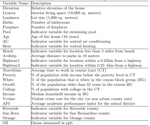
Table 1: Variable Names and Description
Variable Name Description
Elevation Relative elevation of the house
Livarea Interior living space (10,000 sq. meters) Landarea Lot size (1,000 sq. meters)
Baths Number of bathrooms Fireplace Number of fireplaces
Pool Indicator variable for swimming pool Age Age of the house (10 years)
AC Indicator variable for central air conditioning Heat Indicator variable for central heating
Beach Indicator variable for location less than 5 miles from beach Avdistp Average distance to parks in 10 meters
Highway1 Indicator variable for location within a 0.25km from a highway Highway2 Indicator variable for location within 0.25–1km from a highway Traveltime Average time to work in census tract (CT)
Poverty % of population with income below the poverty level in CT White % of the population that is white in the census block group (BG) Over65 % of the population older than 65 years in the census BG College % of population with college in the CT
Income Median household income in BG
Vcrime Violent crime rate for the city (or non urban county rate) API Average academic performance index for the school district Riverside Indicator variable for Riverside county
San Bern. Indicator variable for San Bernardino county Orange Indicator variable for Orange county
OZ Ozone measured in ppb
each house in the city. Where crime rates were not available at the city scale, I use the non-urban crime rate for the county in which the house is located.
A measure of the average school quality is computed from the Academic Per-formance Index (API), published by the California Department of Education.2 This is the primary indicator used by the state to evaluate school performance. The API is an index calculated using both base and growth values of student rankings in the State Standardized tests. It is based on a scale from 200 to 1000 with the target being 800. The average 1999 API value for all schools in a school district is calculated and then assigned to all the houses in the district.3
Besides the beach access variable, three other indicators of accessibility to amenities are included. First, I use the locations for each park in the four counties from the Geographic Names Information System website.4 For each
house location, I then compute the average distance to parks as a summary
2http://www.cde.ca.gov/ta/ac/ap/.
3It would have been preferable to use a measure of school quality from the year previous
to the year in which the house sale takes place, as for the air quality measures. However, information for the API in California school districts is only available starting from 1999.
Figure 1: Spatial distribution of houses and location of monitoring stations.
measure. I also supplement the Census travel time measure with two other indicators of access to the highway system. These are intended to capture both the negative externalities (such as noise) experienced from being very close to the highways, as well as positive externalities due to shorter travel distances. I use ArcGIS and detailed highway maps5 to define increasing buffers of 0.25 km
around the highways and then create two indicator variables. The first takes the value of one if the house is within 0.25 km of a highway, the second takes the value of one if the house is in the buffers that is between 0.25 km and one km from a highway.
Air quality is measured as ambient air pollution. In the literature, hedonic specifications typically include either ozone (OZ) or total suspended particulate matter (TSP) as pollutants, since these are most visible in the form of “smog.” In addition, local news outlets report daily measures of these pollutants and broadcast alerts when dangerous levels are reached. Consequently, it is rea-sonable to assume that pollutants enter into the utility function of potential buyers, although the question remains to what extent a continuous measure of air quality is the appropriate metric.6 I estimate a hedonic model, where OZ
enters as a proxy for air quality.
I use the average of the daily maxima during the worst quarter of 1998 from the hourly observations recorded at monitoring stations for ozone. In
5ESRI Data & Maps CD-ROM. (2002). Redlands, CA: Environmental Systems Research
Institute.
6In Anselin and Le Gallo (2006) discrete categories were also considered. In this paper, I
focus on the functional form of the price-air quality relation and leave the issue of the proper metric for a separate analysis.
Figure 2: Kriging Interpolation: OZ
1998, there were measurements for OZ for 28 monitoring stations. The location of the monitoring stations relative to the houses in the sample is illustrated in Figure (1). This yields a reasonable coverage of the spatial distribution of house locations for OZ.7
I interpolate the values at the monitoring stations to the location of every house in the sample using ordinary kriging. Anselin and Le Gallo (2006) find ordinary kriging to be the most reliable among several interpolation methods, including Thiessen polygons, inverse distance weighting and splines. Figure (2) shows the resulting interpolated values of ozone, with darker color representing higher levels of the pollutant.8 It is interesting to look at the spatial pattern of air pollution measured through ozone. Lower levels are observed closer to the ocean and air quality seems to worsen as one moves North-East with a suggestion of separate air quality “bands.”
The precision of the interpolated value varies across the sample, becoming worse for locations further removed from monitoring sites. To correct for a pos-sible biasing effect of such “high-error” interpolated values, the house locations
7The SCAQMD manages a network of 35 monitoring stations. Only thirty of these stations
monitor OZ levels. Two of this thirty monitors were excluded for purposes of this study because they are located very far away to the east from the location of the houses in the sample. For further detail see www.aqmd.gov/tao/AQ-Reports/2007AQMonitoringNetworkPlan.
8Kriging interpolations were carried out using the ESRI ArcGIS Geostatistical Analyst
extension. A spherical model allowing for directional effects was used for both pollutants. The model chosen included 8 lags with a lag size of 9km, and the estimated parameters were 303.4 and 9 for the direction (angle), 4.16 for the partial sill, 68,604 and 68236 for the major ranges and, 59,381 and 68,236 for the minor ranges.
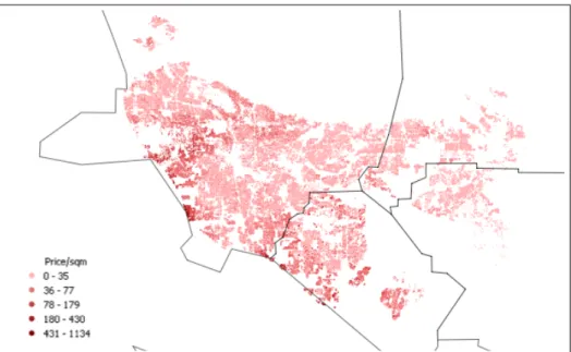
Figure 3: Spatial distribution of house prices (Price/sq.m.)
within the upper 5% of the prediction error distribution for the pollutant were dropped from the sample. This resulted in a final set of 103,867 house locations, of which 67,864 are in LA county, 17,914 in OR county, 12,266 in SB and 5,823 in RI county. The observed sales price ranges from $20,000 to $5,345,455, with an overall mean of $243,346. There is considerable variability across counties. For example, the average house price for observations in LA county is $ 261,946, while it is $269,081 in OR, $148,948 in SB and $146,249 in RI. Figure (3) il-lustrates the spatial distribution of house prices, with higher prices represented through darker colors. Some concentration of high prices per squared meter can be seen in the coast of LA and OR, although overall, there is considerable complexity in the spatial distribution of prices. Basic descriptive statistics for all the variables included in the analysis are given in Table (2).
3
Estimation
I estimate a hedonic function in log-linear form and take an explicit spatial econometric approach. The ultimate objective of this paper is to explore the implications on the estimated MWTP derived from introducing nonlinearities in the relationship between OZ and house prices.
I first obtain ordinary least squares (OLS) estimates for the hedonic model and assess the presence of spatial autocorrelation using the Lagrange Multiplier test statistics for error and lag dependence (Anselin 1988), as well as their robust forms (Anselin et al. 1996).
Table 2: Basic Descriptive Statistics for all Variables
Variable Name Mean Std. Deviation Min Max House Price 243346 210000 20000 5345455 Ln(House Price) 12.213 0.571 9.900 15.490 Elevation 0.995 0.145 -4.000 6.588 Livarea 0.160 0.073 0.050 3.182 Landarea 8.900 19.072 0.8 2818.332 Baths 1.924 0.799 0.500 9.500 Fireplace 0.643 0.560 0 7 Pool 0.150 0.357 0 1 Age 4.287 2.023 0.1 10 AC 0.407 0.491 0 1 Heat 0.277 0.447 0 1 Beach 0.012 0.111 0 1 Pavdist 5.637 0.991 4.447 8.992 Highway1 0.091 0.288 0 1 Highway2 0.342 0.475 0 1 Traveltime 2.936 0.412 1.014 4.717 Poverty 0.120 0.091 0 0.670 White 0.570 0.221 0 1 Over65 0.105 0.059 0 0.868 College 0.259 0.176 0 0.800 Income 5.946 2.588 0 20.000 Vcrime 0.142 0.057 0.037 0.348 API 5.948 0.920 4.271 8.918 Riverside 0.056 0.230 0 1 San Bern. 0.118 0.323 0 1 Orange 0.172 0.378 0 1 OZ 8.111 1.838 4.717 13.467
The results consistently show very strong evidence of positive residual spa-tial autocorrelation, with an edge in favor of the spaspa-tial lag alternative. This matches earlier results obtained in Anselin and Le Gallo (2006) and Anselin and Lozano-Gracia (2008). Formally, a spatial lag model is expressed as:
y=ρW y+Xβ+u, (1) whereyis an×1 vector of observations on the dependent variable,X is an×k
matrix of observations on explanatory variables,W is a n×n spatial weights matrix,uan×1 vector of i.i.d. error terms,ρthe spatial autoregressive coeffi-cient, andβ a k×1 vector of regression coefficients. For further discussion on the theoretical motivation of a spatial lag model see Anselin and Lozano-Gracia (2008). By means of the spatial weights matrixW, a neighbor set is specified for each location. The elements wij of W are non-zero when observations i andj areneighbors, and zero otherwise. By convention, self-neighbors are ex-cluded, such that the diagonal elements ofW are zero. In addition, in practice,
the weights matrix is typically row-standardized, such thatP
jwij = 1. Many different definitions of the neighbor relation are possible, and there is little for-mal guidance in the choice of the “correct” spatial weights.9 The termW y in Equation (1) is referred to as a spatially lagged dependent variable, or spatial lag. For a row-standardized weights matrix, it consists of a weighted average of the values ofy in neighboring locations, with weightswij. In this application, I consider three spatial weights to assess the sensitivity of the results to this important aspect of the model specification. One weight is derived from the contiguity relationship for Thiessen polygons constructed from the house loca-tions. This effectively turns the spatial representation of the sample from points into polygons. The resulting weights matrix is symmetric and extremely sparse (0.006% non-zero weights). On average it contains 6 neighbors for each location (ranging from a minimum of 3 neighbors to a maximum of 35 neighbors, with 6 as the median). I supplement this with two weights matrices based on a nearest neighbor relation among the locations, for respectively 6 and 12 neighbors. The corresponding weights matrix is asymmetric, but equally sparse (respectively 0.006% and 0.012% non-zero weights). The three weights matrices are used in row-standardized form.
In this paper I focus on the estimation of the spatial lag model but allow re-maining spatial error autocorrelation, as well as heteroskedasticity of unspecified form. Following Anselin and Lozano-Gracia (2008) I account for the endogene-ity of the air pollution variable originated from an errors in variables problem. However, I take a step further by allowing a nonlinear relationship between air pollution and house prices.
For this purpose, I estimate a model that no longer imposes the constraint of a functional relationship linear in coefficients, between air quality and house prices (SP-LAGend). As mentioned above this increases the flexibility of the functional form of the hedonic price equilibrium and reduces any biases origi-nating on functional form misspecification. This should in turn result in better estimates of the MWTP for reductions in air pollution. In this case, I esti-mate Equation (10) using a variation of the spatial 2SLS (S2SLS), where the nonparametric function of air quality is estimated using a series approximation (Newey et al. 1999, Pinkse et al. 2002).10
Standard errors are estimated in all cases using the HAC estimator of the covariance matrix as described in Kelejian and Prucha (2006). The HAC being a consistent estimator of the covariance structure under the presence of het-eroskedasticity and autocorrelation of unspecified form, will address any prob-lem stemming from heterogeneity in preferences as well as remaining spatial heterogeneity/autocorrelation. The HAC estimator is of further relevance given that some type of sorting process (that as discussed before is not modeled but
9For a more extensive discussion, see Anselin (2002, pp. 256–260), and Anselin (2006, pp.
909–910).
10The differences deriving from alternative expansion methods have not been explored in
detail in the literature. A comparative study is beyond the aim of the present paper, and it has not been performed because of the computational burden involved by the construction of the expansion terms.
simply relegated to the error term) may lead to heterogeneity.HAC estimates are obtained for three different kernel functions (epanechnikov, triangular and bisquare) to assess the sensitivity of the results to the choice of kernel.
The main advantage of non-parametric methods is that they allow the data to determine which is the most appropriate functional form instead of impos-ing it a priori (Racine and Ullah 2006). As a result, possible estimation biases caused by using an incorrect functional form are avoided. Although it would be desirable to estimate a fully nonparametric function for all variables allowing a fully flexible functional form, this is impractical in most applied work. This problem is known in the literature as thecurse of dimensionality (see Yatchew 2003, for further detail). Hedonic models are usually an example of regressions with large number of explanatory variables, and in the particular case of this paper, a large sample size. In this kind of applications, fully nonparametric mod-els become intractable. Semiparametric methods on the other hand, estimate parametric models but relax some assumptions on functional forms. To this extent, they are less restrictive than parametric approaches. They are useful in cases where fully nonparametric models do not perform well, or when the mean regression is parametric but the form of heteroskedasticity or autocorrelation of the error terms is unknown (Racine and Ullah 2006).
Semiparametric models are extensions of the linear model that introduce more flexibility to the functional form through a nonparametric function. For the linear model,
y=Xβ+, (2)
the most commonly used semiparametric extension is the partially linear model
y=X1β+f(X2) +, (3)
which adds a nonparametric functionf(X2) (Yatchew 2003).
The partially linear model described in Equation (3) has the advantage of controlling parametrically for all other variablesX1, while only a set of variables
X2 are introduced nonparametrically, reducing the curse of dimensionality. In
hedonic models, where it is important to control for many covariates including all house and neighborhood characteristics available, this specification proves to be very useful (e.g. Stock 1989).
Robinson (1988) proposed a “double residual” method to consistently esti-mate the partially linear model described in Equation (3). However, consis-tency of this estimator relies on the assumption of independence offrom X1
andX2. Newey et al. (1999) introduce a consistent semiparametric estimator in
the presence of endogenous regressors. ForX2 endogenous, the authors assume
f(X2) lies in a compact set of functions. Newey et al. (1999) suggest that the
structural functionf(X2) may be approximated by a function which is linear
in parameters, such as:
f(X2) =
J
X
l=0
αlel(X2) (4)
where the el are basis functions which provide a good approximation for
polynomial (like Taylor Series or Legendre polynomials) and spline approximat-ing functions. An extension of this endogeneity corrected series estimator to the spatial context is laid out in Pinkse et al. (2002). Pinkse et al. (2002) provide a consistent estimator of a semiparametric spatial lag model. The semipara-metric extension of the spatial lag model, presented in Pinkse et al. (2002) that introduces the neighboring relations nonparametrically looks as follows:
y=Gy+Xβ+u, (5)
whereGis ann×nmatrix with zero diagonal elements and off diagonal elements
gij=g(dij) whereg(dij) is an unknown function that must be estimated anddij is some measure of distance between observationsiand j. The functiong(dij) can be considered the nonparametric equivalent to a spatial weights matrix in the fully parametric case. As expressed by Pinkse et al. (2002), it is possible to have a range of different definitions fordij. Without loss of generality, one can assume for example that the elementsdij are formed by a compound of discrete measuresdDij and a vector of continuous distance measures dcij. Following this definition, the nonparametric function of distancesg(d) can be written as:
g(d) =
∞
X
i=1
I(dD=t)gt(dc), (6)
whereI is an indicator function that takes the value of one when its argument is true and zero otherwise. For example, the condition could be that the two spatial units share a common border (rook criterion) or a point (queen criterion). The functionsgt(dc) can in turn be written as,
gt(dc) = ∞
X
i=1
αtletl(dc), (7)
wheret= 1, ...D∗are the numbers of dichotomous indicators included.
As suggested by Newey et al. (1999), Pinkse et al. (2002) use a series-expansion approach to estimategt(dc). Pinkse et al. (2002) use trigonometric functions and in particular, Legendre polynomials. Equation (5) may now be rewritten as follows,
y=Aα+Xβ+, (8)
where α = [α1, ..., αLB]0 are coefficients to be estimated, LB is the number of expansion terms included; A is an N ×LB matrix whose (i, l) element is
P
i6=jel(dij)yj and is the error term that includes the expansion terms that were not estimated, taking the form,
=u+
∞
X
l=Lb+1
αlel(d)y (9)
Given the presence of the dependent variable on the right hand side, Equa-tion (8) must be estimated using an Instrumental Variables approach. Pinkse
et al. (2002) suggest to instrument the functionP∞
l=1αlglyusingPi=6 jel(dij)Xj. Each explanatory variable in X providesLB additional instruments.
An alternative specification of equation (5) where the weights are intro-duced parametrically, but an additional endogenous regressory2 is introduced
nonparametrically would be written as follows:
y=ρW y+Xβ+h(y2) +u (10)
I explore the nonlinearities in the relationship between OZ and house prices by estimating Equation (10) using Pinkse et al. (2002) estimator. Therefore, the model presented in Equation (10) is the focus of this paper. Specifically, for this applicationy represents a vector ofn×1 log of house prices, X is an
n×kmatrix of exogenous regressors,W is an×nspatial weights matrix,y2is
a vector ofn×1 measures of air pollution (Ozone),uis a vector ofn×1 i.i.d. error terms, ρis the spatial autoregressive coefficient, and β is a k×1 vector of regression coefficients. This model presents endogeneity from two sources. First, the dependent variable that appears on the right hand side through the spatial lag of prices. Second, an additional endogenous variable y2. For this
particular case, the conditions for consistency described in Pinkse et al. (2002) remain unchanged and therefore Equation (10) can be estimated following sim-ilar steps as described above. The spatial lag is instrumented using the spatial lag of the explanatory variablesW X. This choice is based on the reduced form of the model and has been widely discussed in the literature (Anselin 1980, 1988, Kelejian and Robinson 1993, Kelejian and Prucha 1998, 1999, Kelejian et al. 2004, Lee 2003, 2006). Furthermore, the function P∞
l=1αlhl(y2) may be
instrumented usingP∞
l=1αlhl(Z), whereZ is some instrument fory2. As
men-tioned in Pinkse et al. (2002), ifZexplains variation inythen one would expect
P∞
l=1αlhl(Z) to explain most of the variation in
P∞
l=1αlhl(y2). In estimating
the standard errors of the coefficients it is important to recall thatin Equation (8) includes neglected expansion terms and therefore it is heterogeneous by con-struction. Pinkse et al. (2002) suggest a generalization of the Newey and West (1987) estimator, where the covariance matrix is estimated in the following way:
ˆ
Ψ =n−1Q0ΣˆQ, (11) whereQis a matrix of uniformly bounded variables (such as the set of regres-sors), ˆΣij is the generic element of the matrix ˆΣ such that ˆΣij =aijµˆiµˆj and
aij are weights that, for fixed i and j converge to 1 as N increases. Pinkse et al. (2002) suggest using weights such that aij = 1 if i is among j’s four nearest neighbors11 AND j is among i’s four nearest neighbors; a
ij = 0.5 if i is amongj’s four nearest neighbors OR j is among i’s four nearest neighbors, and aij = 0 otherwise. However, the conditions in the model do not provide any guidance on the most efficient choice for such weights as is recognized by the authors. The selection of weights used in Pinkse et al. (2002) seems a bit arbitrary. The recently developed heteroskedastic and autocorrelation consis-tent (HAC) estimator for the variance covariance matrix developed in Kelejian
and Prucha (2006), is a particular form of the covariance estimator in Equa-tion ( 11). The main difference being that in the HAC estimator the weights are assigned through a kernel function of the distances between each pair of observations (see Equation ( 12)).
b ψr,s= (1/n) X i X j qirqjsuˆiuˆjK(dij/d), (12)
Choosing to assign the weights through a kernel function in the form of the HAC estimator instead of arbitrarily assigning weights with some a priori crite-rion as in Pinkse et al. (2002), the advantages of a nonparametric specification are exploited again in the estimation of the variance covariance matrix.
4
Empirical Results
I begin the review of the empirical results by focusing on the coefficients of the parametric models that define a baseline for the semiparametric models, which are the main focus of this paper. The parametric methods under con-sideration are: OLS, IV (standard non-spatial 2SLS with air pollution treated as endogenous), LAG-end (spatial 2SLS with a spatially lagged dependent vari-able and the pollutant treated as endogenous). The model that accounts for a nonlinear relationship between air pollution and house prices is estimated using two alternative semiparametric estimation methods: semiparametric IV (SP-IV, pollutants treated as endogenous and introduced through a nonparametric function) and semiparametric LAG-end (SP-LAGend, spatial lag model with pollutant treated as endogenous and introduced through a nonparametric func-tion). Estimated coefficients are shown in Table (3). Although IV estimates are inconsistent both in parametric and semiparametric specifications, I present them here for comparison purposes.
First, consider the OLS results. Overall, the coefficients of the house char-acteristics are significant and of the expected sign, in accordance with earlier findings in the literature. The only exception is relative elevation, which was not found to be significant. House prices increase as both land and living area increase. Similarly, houses with more bathrooms, fireplaces, and heating sys-tems are higher valued. As the literature suggests (see Bourassa et al. 1999, Beron et al. 2004, among others) there appears to be a quadratic relationship between age and price: prices are higher for more recently built houses. There is also avintage effect of age on prices that is reflected in the positive sign of the quadratic term.
In terms of access variables, there is a significant premium for houses that are located closer to the beach and closer to parks, but the effect of the immediate vicinity to the highway is that of a nuisance. Location in a zone 0.25 to 1km from the highway is not significant.
The results for the neighborhood variables are also in accordance with con-ventional wisdom: travel time and crime are negatively valued, whereas % white, the proportion of college graduates and median income have a positive effect.
Poverty and the school quality score were not found to be significant. The per-centage elderly is positive, but its significance is not stable across estimators (see below).
Los Angeles county was used as the base case, which resulted in a nega-tive value for the dummy variables for Riverside and San Bernardino, but no significant difference for Orange county.
The overall fit is very satisfactory, with anR2of 0.77. However, as the model
diagnostics indicate (bottom part of Table (3)), OLS suffers from a number of problems. First, the Durbin-Wu-Haussman (DWH) test statistic for endogene-ity strongly rejects the null hypothesis that the interpolated pollutant is exoge-nous. In addition, there is evidence of very high residual spatial autocorrelation, with the robust LM test statistic (RLM-lag and RLM-err) suggesting the lag specification as the proper alternative (Anselin et al. 1996) .
I next consider the effect on the estimates for the traditional hedonic vari-ables of treating the pollutants as endogenous (column IV in Table (3)), and combining both spatial lag and endogeneity of the pollutants (column LAG-end). Note that the Anselin and Kelejian (1997) (A-K) test for residual spatial autocorrelation also rejects the null for the IV estimates. The hypothesis is not rejected when both spatial lag and endogeneity of the pollutants are consid-ered. The most appropriate specification is therefore the LAG-end. The results for the OLS, IV, and SP-IV especifications are provided to assess the effect of addressing endogeneity and spatial effects in isolation vs. in combination.
For the individual house characteristics and accessibility variables, the es-timated coefficients remain fairly stable across methods, with only marginal changes. The estimates obtained with LAG-end are slightly smaller in abso-lute value, but the significances remain the same. This is not the case for the estimates of the neighborhood characteristics. These vary considerably across methods, both in magnitude as well as in significance. For example,the absolute value of the coefficients for Income, College and Vcrime in LAG-end is about half (or even less in some cases) the magnitude for OLS. Percentage of elderly becomes significant only at the 5% level for the LAG-end. These variables are measured at an aggregate scale (census tract or block group, or city for the crime variable) and therefore the disturbances from the model may be corre-lated within the aggregation groups (Moulton 1990). It is likely that houses in the same census tract share unobservable characteristics leading to correlation in the error terms. I surmise that the inclusion of a spatially lagged dependent variable filters out some of this error and yields more accurate estimates.
The pollution variables are similarly affected by the estimation method. Ozone coefficients are negative and highly significant throughout. However, their absolute value varies considerably across methods. Taken individually, the effect of controlling for endogeneity seems to be strongest, resulting in a change between OLS and IV from−0.041 to−0.051. In LAG-end, accounting for both spatial effects and endogeneity yields a coefficient of −0.033 for Ozone. This suggests that a reduction of 1 ppb in OZ levels would raise house prices by 3%. Interestingly, the A-K test in the LAG-end model shows evidence of signif-icant remaining spatial error autocorrelation for the knn-6 and knn-12 but not
for the queen weights. I compute three sets of standard errors (classical, White (heteroskedastic consistent), and HAC) to assess the effect of the presence of remaining spatial autocorrelation and heteroskedasticity on the precision of the estimates. The results are reported in Tables (5) in the Appendix , for the three spatial weights matrices and three kernel functions.
The estimates for the pollution variable are essentially the same across the three spatial weights. However, accounting for remaining heteroskedasticity and spatial error correlation has a dramatic effect on the precision of the estimates. The standard errors are up to twice as large for the HAC as the classical and White results with consistently the largest value for the Epanechnikov kernel. By and large, the numerical values are essentially the same across kernels and spatial weights, which provides some evidence of the robustness of the findings. The more realistic measure of the standard errors of the estimates will be im-portant in assessing the precision of the derived welfare measures, such as the MWTP, to which I will turn in the next section.
Moving on to the semiparametric specification, I compare the “best” model (SP-LAGend) to the non-spatial model (SP-IV ). Such a comparison will con-tribute to the understanding of the effect of including space in a semiparametric context. Both semiparametric models are estimated using the Pinkse et al. (2002) estimator. Significance of the coefficients in Table (3) corresponds to HAC standard errors with an Epanechnikov kernel.12 Comparing estimates from
SP-LAGend to estimates from SP-IV suggests that the introduction of space in the semiparametric specification has an effect mainly on the magnitude of the coefficients but not in their significance. As it was the case in the parametric specifications, larger changes in magnitude are observed for the variables that represent characteristics at the aggregate level. Therefore, the spatially lagged dependent variable appears to be filtering out some of the error originated in the high level of aggregation of some explanatory variables, leading to better estimates.
Let us now take a closer look at the comparison between parametric and semiparametric spatial specifications (LAGend and SP-LAGend). It is interest-ing to notice how for the individual house characteristics and accessibility vari-ables, the estimated coefficients remain fairly stable across methods, with only marginal changes. The estimates obtained with LAG-end are slightly smaller in absolute value, but all the significances remain the same. Coefficients for house characteristics are very close in magnitude and significance to their parametric counterpart, LAG-end. As it was the case for the parametric models, larger changes occur for variables measured at an aggregate scale. Poverty, which was not significant in the parametric models, becomes significant and of the expected sign in the SP-LAGend model. Estimates for both highway variables in the SP-LAGend are consistent with the results for the LAGend parametric model. Larger changes in magnitude and significance are seen when endogeneity of air pollution is introduced rather than when moving from a parametric to a
12Results for triangle and bisquare kernels are consistent and available from the author
Table 3: Coefficient Estimates: OZ Model– Queen Weights
Variable Name OLS IV LAG-end SP-IV SP-LAGend Constant 11.8051 11.8657 7.1140 133.395 24.046 Landarea 0.0011 0.0012 0.0009 0.0010 0.0008 Elevation 0.0025* 0.0040* 0.0061* -0.0206* 0.0016* Livarea 2.6229 2.6240 2.1654 2.6284 2.1567 Baths 0.0472 0.0474 0.0405 0.0602 0.0418 Fireplace 0.0473 0.0475 0.0355 0.0596 0.0368 Pool 0.0511 0.0526 0.0436 0.0618 0.0437 Age -0.0142 -0.0147 -0.0110 -0.0454 -0.0153 Age2 0.0225 0.0229 0.0153 0.0730 0.0221 AC -0.0245 -0.0206 -0.0117 -0.0585 -0.0200 Heat 0.0412 0.0422 0.0237 0.0577 0.0243 Beach 0.2107 0.1969 0.1319 0.3999 0.1670 Distance Parks -0.0172 -0.0131 -0.0105 0.0066* -0.0050 Highway1 -0.0176 -0.0188 -0.0108 -0.0169* -0.0121 Highway2 0.0023* 0.0013* 0.0038* -0.0041* 0.0017* Travel time -0.0693 -0.0667 -0.0532 -0.2082 -0.0783 Poverty 0.0431* 0.0405* -0.0111* -0.3050** -0.0578* White 0.3301 0.3349 0.2152 0.4482 0.2285 Over65 0.1766 0.1765 0.0553** 0.4483 0.0996 College 1.0962 1.0931 0.5592 1.3289 0.5819 Income 0.0199 0.0194 0.0047 0.0130 0.0032 Vcrime -0.5767 -0.6743 -0.3780 -2.5688 -0.5414 API 0.0007* 0.0011* 0.0019* -0.0836 -0.00855 Riverside -0.2440 -0.2184 -0.1386 0.3898 -0.0297* Orange -0.0699 -0.0802 -0.0574 0.2310 -0.0043* San Bern. -0.1914 -0.1655 -0.1009 0.2958 -0.0047* Ozone -0.0411 -0.0515 -0.0336 (See Figures 4 and 5 )
Wlnpx — — 0.4011 — 0.4081 RLM-LAG 2357.271 — — — RLM-ERR 1339.671 — — — DWH 2540 — — — A-K — 16889.31 0.09 R2 (corr): 0.77176 0.7713 0.77612 0.50455969 0.75199187 * Not significant ** Significant at 5 percent semiparametric specification.
The spatial coefficient is very significant and of similar magnitude in both parametric and semiparametric specifications. Figure 4 illustrates the biases that would arise form ignoring space in the semiparametric model. It compares the price response from the SP-IV estimator to the direct effect obtained through the SP-LAGend estimator. Using the standard errors from the more appropriate SP-LAGend estimator we see that the price response functions are statistically different from each other for most OZ levels. In other words, the SP-IV response
Figure 4: Price Response SP-IV and SP-LAGend
function (red line) lies outside the 95% confidence interval for the SP-LAGend response function, defined by the orange and green lines. Furthermore, the semiparametric model gives an average change in prices of 2% for a reduction of 0.1ppb in OZ levels, while the spatial estimate suggests an average response of 0.6%. In absolute value, the SP-IV would in general suggest a larger price response than the SP-LAGend. However the magnitude of that bias changes across OZ levels. One explanation for this difference may be that the spatial effect is being filtered out at a local scale with respect to the pollutant. Therefore different effects on the curvature of the price response function are observed along the X-axis, when moving from the non spatial IV to the spatial SP-LAGend. This will have an effect on the local (with respect to OZ) estimates of the MWTP.
It is important to remember that given the presence of a spatially lagged dependent variable the SP-IV estimate is biased and inconsistent. As a conse-quence, its price response function is higher (in absolute value) for both small and high levels of ozone than the one implied by the consistent SP-LAGend estimate. As seen in Figure (4), SP-IV estimator would in general give a higher price response of the effect of changes in air pollution as would the IV estimate in the fully parametric case. The estimated price response to a change of 0.1ppb in ozone levels for the SP-LAGend models is shown in Figure (5).13 In Figure
13All graphs, unless otherwise noted, are obtained using the lowess graphical function in
Figure 5: Price Response for a Decrease of 0.1 ppb in OZ - SP-LAGend Model, Direct vs Multiplier Effect
(5), the blue line is the actual price response function including the Multiplier effect, while the red line shows the price function only for the Direct effect. The horizontal axis of this Figure reports the different levels of OZ. The price response function gives a way to illustrate the estimated series approximation of the nonparametric function of ozone. The yellow and green lines represent the upper and lower bounds of a 95% point-wise confidence interval.14 The hor-izontal (grey) line was drawn in correspondence to the value of the coefficient for ozone from the respective parametric model (Multiplier effect).
It appears immediately evident from the graph that the highest variations in prices are concentrated at locations with smaller as well as higher levels of ozone. For values of ozone between 8 and 11 ppb the price response function from the semiparametric spatial specification gets very close to the value of the coefficients from the parametric model. Figures (5) and (4) suggest that the effect on prices decreases as OZ levels increase. Smaller price changes will be observed in houses located in relatively more polluted areas. Furthermore, it is interesting to see that the change in prices might even be negative for the highest levels of pollution, i.e. prices will decrease when air pollution decreases. For middle range levels of ozone, say between 8 and 11 ppb, the response function
the sample.
14To obtain these confidence intervals I use an approximation where I evaluate the function
estimated using the SP-LAGend is almost flat, indicating that for this range, the relationship between house prices and OZ is close to linear. In addition, the response appears to be very close to zero -but still statistically different from zero, for this range. Figure (5) also shows how ignoring the Multiplier Effect would lead to underestimation of the price response for most OZ levels. The direct effect (red line) falls below the multiplier effect for all levels of ozone under 12ppb. Furthermore, only for OZ levels between 7 and 8.5 do the two effects do not appear to be statistically different from each other. Parametric models on the other hand, suggest a constant price response across all pollution levels (grey line). Figure (5) also suggests that looking at a parametric model will lead to an average response function that in general suggests a lower effect on prices. In other words, the average effect estimated from a parametric model is being driven by the lower effects that only part of the population experiences. In general, it is clear that linear models provide an average of the variation of price responses across pollutant levels. The linear model appears to be a good approximation for middle range pollution levels but it hides the real effects at the extremes, both in low and highly polluted areas, which is also where differences in prices are more substantial. Of course, nonlinearities originating in the nonparametric part of the hedonic equation not only affect the way we look at the relationship between air quality and house prices. As expected, these nonlinearities are carried over to the MWTP. The following section is devoted to the analysis of the impact of nonlinearities in the hedonic price equation on the MWTP.
5
Marginal Willingness to Pay and Policy
Anal-ysis
Using estimates obtained in the previous section it is possible now to estimate the MWTP for reductions in air pollution that results from each model esti-mated. I can now assess the impact that introducing nonlinearities in ozone will have on the valuation of air quality.
In a non-spatial log-linear model, the MWTP equals the estimated coefficient for the pollution variable times the price (P) as shown in Equation (13).
\
M W T POZ=
∂P
∂OZ =βdOZP, (13)
However, as suggested by Kim et al. (2003), an additional term called the Mul-tiplier Effect appears when the MWTP is derived for a spatial lag model and the MWTP takes the following form:
\ M W T POZ= ∂P ∂OZ =βdOZP( 1 1−ρb), (14)
For the SP-LAGend, the MWTP for a reduction in OZ levels would take yet another form. For the SP-LAGend model, both direct an Multiplier Effects
Figure 6: Marginal Willingness to Pay for a 0.1 Reduction in OZ, SP-LAGend
would involve the derivative of the nonparametric function of OZ, h(y2) (see
Equation (10)). The Multiplier effect for the SP-LAGend model is laid out in Equation (15). \ M W T POZ= ∂P ∂OZ = \ ∂g(OZ) ∂OZ P( 1 1−ρb), (15)
Figure (6) depicts both the direct and Multiplier Effects of the marginal willingness to pay for an improvement in air quality, measured through a re-duction of 0.1 ppb in OZ from the SP-LAGend. The MWTP for changes in OZ levels appears to be in general positive suggesting that households are willing to pay up to about 9% the price of the house for a 0.1 ppb decrease in OZ levels.15 However, for most Ozone levels the MWTP seems to be much lower, being close to the parametric estimates. The dark red and blue horizontal lines show re-spectively the Multiplier and Direct Effects estimated from a fully parametric model. These estimates are all depicted as a percentage of prices for a reduction of 0.1 ppb in OZ levels. The grey and light red lines give the MWTP as a per-centage of price (Multiplier and Direct Effects) estimated from the SP-LAGend model. As it is was the case in the parametric models, the Multiplier Effect is larger (in absolute value) than the Direct Effect for all OZ levels. However, this difference does not appear to be significant for OZ levels between 7.5 and 8.5 or
15Recall that the MWTP reflects capitalized values of the benefits associated with
higher than 12.16 The linear model appears to be a good approximation only for areas with middle levels of pollution where the linear estimates lie between the 95% confidence interval for the Multiplier Effect from the SP-LAGend model. However, for lower levels of pollution the linear model provides a misleading estimate of the marginal willingness to pay.
At this point it is important to discuss the shape of the relationship between MWTP and OZ levels. Note that the X-axis measures a “bad” and therefore the shape depicted in Figure (6) would suggest an increasing MWTP which would violate the assumption of non-increasing marginal utilities. However, if there is heterogeneity of preferences with respect to ozone, and individuals sort according to such heterogeneity, then the increasing marginal utility in air qual-ity would be consistent with negative assortative matching (i.e. individuals who prefer cleaner air sort into locations with better air quality)17. In other words, in
a nonlinear model, testing for heterogeneity in preferences becomes particularly important. If preferences are homogeneous with respect to the characteristic being analyzed, then nonlinearities in the hedonic price equilibrium will allow the complete identification of the demand function. One would have exactly the WTP for each level of the characteristic observed. On the other hand, if preferences are heterogeneous with respect to that characteristic one would find as many WTP functions as heterogeneous groups and will only be able to identify as many points of each bid function as individuals in each group. If there are heterogeneous preferences, the value of nonlinear models is that they provide local estimates with respect to the characteristic being analyzed, rather than an average MWTP than in the heterogeneous case might reflect the WTP of a sub-population. If there are homogeneous preferences then the advantage of nonlinear models is that they allow you to fully identify the bid (MWTP) function.
Eubank and Thomas (1993) propose the use of residual plots as a diagnostic tool for detecting heteroskedasticity related to an explanatory variable, which in the present case would be OZ. As stated by Eubank and Thomas (1993), a wedge shape pattern in a plot of residuals against the variable (or a transforma-tion of it) would be indicative of heteroskedasticity. If there is no heterogeneity with respect to OZ, regression residuals should not show any pattern when plot-ted against OZ levels. However, Figure (7) suggests a trend where residuals increase as OZ levels increase. The positive slope of the curve for low levels of pollution indicates negative assortative matching. For middle to high levels of air pollution tastes heterogeneity appears to be less of a problem. Given that heterogeneity of preferences appears to be present in this example, the estimated MWTP shown in Figures 6 does not identify the MWTP function but instead local MWTP estimates with respect to OZ. As discussed above, each point in the curve represents a point in a particular bid function for the preferences associated with each OZ level. Therefore it becomes particularly
16Higher and lower bounds for a 95% confidence interval for the Multiplier Effect (orange
and green lines in Figure (6) are obtained using HAC standard errors with an Epanechnikov kernel.
Figure 7: SP-LAGend Residuals
interesting to compare these “local” estimates with the “global” estimates ob-tained from parametric models. This is clearly expressed in Figure (8) which depicts the estimated MWTP from a SP-LAGend specification. It is clear that estimated MWTP varies by location and it follows a pattern similar to that of OZ. Contrasting Figures (8) and (2) one can observe that lowest levels of esti-mated MWTP (in some cases even negative) appear in areas with middle range pollution levels, with a few houses at the North-East being located in more polluted areas. These lowest valuations which refer to negative MWTP levels are seen in the lighter blue band that appears in the middle of the sample as well as for some houses in the north east corner. Apparently, to the South-West of that band individuals sort with respect to air pollution. Higher valuations are seen in areas with lowest air pollution level so that people who have higher preferences for air pollution are choosing homes in less polluted ares. On the other hand, to the North-East of the light blue band we see that estimated MWTP appears to increase as pollution increases. This behavior is consistent with the non-increasing marginal utility and will therefore suggest that sorting with respect to air pollution does not take place in this area of the SCAB region. Estimates from linear models will tend to reflect the willingness to pay of subpopulations. Extrapolating the estimated household MWTP for changes in air quality for all the population living in the area, it becomes clear that a parametric model underestimates the aggregate MWTP for the region. To do this, I used population data at the census tract level from the Census 2000.
Figure 8: SP-LAGend Estimated MWTP as a % of Price
Multiplying the average MWTP at the census tract for the number of households in that census tract and then averaging over all census tracts in the sample (2418 census tracts) I obtained total WTP for marginal changes in air pollution. Total values represent the sum of the MWTP of all tracts.
Table (4) suggests that the total aggregate WTP for a reduction of 0.1 ppb in ozone levels would be considerably smaller when using a fully parametric model than when using the more flexible semiparametric model. The difference between the two estimates would be over 1.5 billion dollars for the Direct Effect and about 3 billion dollars for the Multiplier Effect. The aggregate estimates from a fully parametric model are about a third of the estimates from a semi-parametric model. More problematic is the fact that a semi-parametric specification suggests that for all households in the sample the MWTP is positive, giving a minimum aggregate MWTP (by census tract) of almost $ 18,000. The aggre-gated estimates shown in Table 4 are in line with those from previous work. In particular, Brucato et al. (1990) estimate aggregate benefits from a 10% reduction in ozone levels to be between 320 and 530 million dollars (in 1984 dollars) using house sales taking place between 1978 and 1979 in San Francisco. Although they do not report the number of households these numbers pertain to, there were around 299.867 households in San Francisco in 1980. Converted to 2005 dollars, this would represent a benefit ranging between 800 and 1,325
Table 4: Total MWTP Non-Spatial Models OLS IV Mean 2,022,993 1,614,466 Min 21,872 27,406 Max 17,400,000 21,800,000 Total 3,990,000,000 4,890,000,000 Spatial Models - LAGend
Direct Effect Multiplier Effect Parametric Model Mean 1,320,033 2,204,317 Min 17,880 29,840 Max 14,200,000 23,700,000 Total 3,190,000,000 5,330,000,000 Semiparametric Mean 2,052,613 3,465,467 Min -11,200,000 -18,900,000 Max 43,700,000 73,800,000 Total 4,960,000,000 8,380,000,000 3,869,817 households
million dollars. Converting the 1999 values presented in Table 4 would in turn suggest aggregate mean benefits ranging between 5,835 and 9,860 for the semi-parametric models and between 3,752 and 6,270 million dollars for the fully parametric models.
6
Conclusions
The contribution of this paper to the literature on valuation of air quality in the context of spatial hedonic models is twofold. First, I consider the possibility of two types of nonlinearities in the hedonic price function that may affect the estimation of the MWTP for reductions in air pollution. This led to the use of nonparametric methods for the estimation of the hedonic equilibrium. Besides addressing nonlinearities this also considered endogeneity of two sources: the presence of the spatially lagged dependent variable and the errors in variables problem highlighted in Anselin and Lozano-Gracia (2008). Second, I implement semiparametric methods in the context of a spatial lag model which have not been applied before in the valuation of non-market goods using hedonic models. The results I present in this paper highlight the need to allow for nonlineari-ties in air pollution within a hedonic specification. However, nonlinearinonlineari-ties in the neighborhood definition do not appear to have a strong effect on the estimates of the MWTP when compared to the fully parametric case. As it is the case in the parametric models, in the semiparametric specification the effects from accounting for spatial autocorrelation on house characteristics are minimal. On
the other hand, air pollution as well as neighborhood characteristics estimates are considerably affected by the introduction of a spatially lagged variable. The estimates are affected both in magnitude and significance and the biases on the price response from ignoring spatial autocorrelation vary across pollution levels. Nonlinearities with respect to OZ defined in the hedonic price equilibrium are transfered into nonlinearities of the estimated MWTP. For middle-low levels of air pollution, linear models seem to provide a close approximation to the estimates from semiparametric models. Furthermore, the difference between Multiplier and Direct Effects becomes insignificant for such levels of pollution.
At an aggregate level, the consequences from imposing linearity in the he-donic price equilibrium become more clear. Given the population distribution in the SCAB, aggregate measures from linear models will tend to reflect the willingness to pay of only those living in areas with middle levels of pollution (8 ppb for OZ ) considerably underestimating the MWTP of those living in less polluted areas.
By introducing nonlinearities in the hedonic price equilibrium the problem of heterogeneity in preferences with respect to OZ emerges. This problem was only identified in this paper and including such heterogeneity in the structural model should be the objective of future work. The results from the semiparametric models allows us a glance into what the results for a model that accounts for heterogeneity would look like. Explicitly modeling such heterogeneity might pro-vide further insight into the functional form of the MWTP for sub-populations that sort with respect to pollution levels.
T ab le 5: St andar d Er rors: OZ Co eff. Standard E rrors OZ Class ical White H A C-Ep HA C -T r HA C-Bi OL S -0. 04109 0. 00077 0. 000821 0. 00179 0 .001574 0.001 60 IV -0. 05150 0. 000816 0. 000822 0. 00197 0.00173 0.001 764 LA G Q ueen -0. 029899 0. 00074218 0. 00085196 0. 001297 49 0.0011 9342 0.001 18481 LA G-end -0. 03357 0. 00078317 0. 00092164 0. 001343 51 0.0012 3449 0.001 24219 LA G Knn6 -0. 02857 0. 00073816 0. 00087357 0. 001297 36 0.0011 8687 0.001 19365 LA G-end -0. 03225 0. 00078076 0. 00095066 0. 001358 62 0.0012 4997 0.001 25604 LA G Knn12 -0. 02783 0. 00073675 0. 00085930 0. 001266 92 0.0011 7507 0.001 16825 LA G-end -0. 03113 0. 00077790 0. 00093162 0. 001332 85 0.0012 3551 0.001 24214
References
Anglin, P. M. and Gencay, R. (1996). Semiparametric estimation of a hedonic price function. Journal of Applied Econometrics, 11:633–648.
Anselin, L. (1980). Estimation Methods for Spatial Autoregressive Structures. Regional Science Dissertation and Monograph Series, Cornell University, Ithaca, NY.
Anselin, L. (1988). Spatial Econometrics: Methods and Models. Kluwer Aca-demic Publishers, Dordrecht, The Netherlands.
Anselin, L. (1998). GIS research infrastructure for spatial analysis of real estate markets. Journal of Housing Research, 9(1):113–133.
Anselin, L. (2002). Under the hood. Issues in the specification and interpretation of spatial regression models. Agricultural Economics, 27(3):247–267.
Anselin, L. (2006). Spatial econometrics. In Mills, T. and Patterson, K., editors, Palgrave Handbook of Econometrics: Volume 1, Econometric Theory, pages 901–969. Palgrave Macmillan, Basingstoke.
Anselin, L., Bera, A., Florax, R., and Yoon, M. (1996). Simple diagnostic tests for spatial dependence. Regional Science and Urban Economics, 26:77 104. Anselin, L. and Kelejian, H. H. (1997). Testing for spatial error
autocorrela-tion in the presence of endogenous regressors. International Regional Science Review, 20:153–182.
Anselin, L. and Le Gallo, J. (2006). Interpolation of air quality measures in hedonic house price models: spatial aspects.Spatial Economic Analysis, 1:31– 52.
Anselin, L. and Lozano-Gracia, N. (2008). Errors in variables and spatial effects in hedonic house price models of ambient air quality. Empirical Economics, 34:5–34.
Basu, S. and Thibodeau, T. G. (1998). Analysis of spatial autocorrelation in house prices. Journal of Real Estate Finance and Economics, 170(1):61–85. Beron, K. J., Hanson, Y., Murdoch, J. C., and Thayer, M. A. (2004). Hedonic
price functions and spatial dependence: Implications for the demand for urban air quality. In Anselin, L., Florax, R. J., and Rey, S. J., editors,Advances in Spatial Econometrics: Methodology, Tools and Applications, pages 267–281. Springer-Verlag, Berlin.
Bourassa, S., Hamelink, F., Hoesli, M., and MacGregor, B. (1999). Defining residential submarkets. Journal of Housing Economics, 8:160–183.
Boyle, M. A. and Kiel, K. A. (2001). A survey of house price hedonic studies of the impact of environmental externalities. Journal of Real Estate Literature, 9:117–144.
Brasington, D. M. and Hite, D. (2005). Demand for environmental quality: a spatial hedonic analysis. Regional Science and Urban Economics, 35:57–82. Brucato, P. F. J., Murdoch, J., and Thayer, M. A. (1990). Urban air quality
im-provements: a comparison of aggregate health and welfare benefits to hedonic price differentials. Journal of Environmental Management, 30:265–279. Chay, K. Y. and Greenstone, M. (2005). Does air quality matter? evidence
form the housing market. Journal of Political Economy, 113(2):376–424. Clapp, J., Kim, H.-J., and Gelfand, A. (2002). Predicting spatial patterns of
house prices using LPR and Bayesian smoothing. Real Estate Economics, 30:79–105.
Cropper, M. L., Decl, L. B., and McConnell, K. E. (1988). On the choice of func-tional form for hedonic price functions. Review of Economic and Statistics, 70:668–675.
Dubin, R., Pace, R. K., and Thibodeau, T. G. (1999). Spatial autoregression techniques for real estate data. Journal of Real Estate Literature, 7:79–95. Ekeland, I., Heckman, J. J., and Nesheim, L. (2004). Identification and
estima-tion of hedonic models. Journal of Political Economy, 112(1):S60–S109. Eubank, R. L. and Thomas, W. (1993). Detecting heteroscedasticity in
nonpara-metric regression. Journal of the Royal Statistical Society, Series B (Method-ological), 55(1):145–155.
Freeman, A. M. I. (1974). Air pollution and property values: A further comment. Review of Economics and Statistics, 56(4):415–416.
Gencay, R. and Yang, X. (1996). A forecast comparison of residential hous-ing prices by parametric and semiparametric conditional mean estimators. Economic Letters, 52:129–135.
Gillen, K., Thibodeau, T. G., and Wachter, S. (2001). Anisotropic autocor-relation in house prices. Journal of Real Estate Finance and Economics, 23(1):5–30.
Gress, B. (2004). Using semi-parametric spatial autocorrelation models to im-prove hedonic housing price prediction. Working Paper UC Riverside Eco-nomics Department.
Harrison, D. and Rubinfeld, D. L. (1978). Hedonic housing prices and the demand for clean air.Journal of Environmental Economics and Management, 5:81–102.
Hartog, J. and Bierens, H. (1991). Estimating a hedonic earnings function with a nonparametric method. In Ullah, A., editor, Semiparametric and nonparametric econometrics: studies in empirical economics. Springer, Berlin Heidelberg New York.
Iwata, S., Murao, H., and Wang, Q. (2000). Nonparametric assessment of the effects of neighborhood land uses on the residential house values. In Fomby, T. and Carter Hill, R., editors,Advances in econometrics: Applying Kernel and nonparametric estimation to economic topics, volume 14. JAI Press, New York.
Kelejian, H. H. and Prucha, I. R. (1998). A generalized spatial two-stage least squares procedure for estimating a spatial autoregressive model with autoregressive disturbances. Journal of Real Estate Finance and Economics, 17(1):99–121.
Kelejian, H. H. and Prucha, I. R. (1999). A generalized moments estimator for the autoregressive parameter in a spatial model. International Economic Review, 40(2):509–533.
Kelejian, H. H. and Prucha, I. R. (2006). HAC estimation in a spatial framework. Journal of Econometrics. Forthcoming.
Kelejian, H. H., Prucha, I. R., and Yuzefovich, Y. (2004). Instrumental variable estimation of a spatial autoregressive model with autoregressive disturbances: Large and small sample results. In LeSage, J. P. and Pace, R. K., editors, Advances in Econometrics: Spatial and Spatiotemporal Econometrics, pages 163–198. Elsevier Science Ltd., Oxford, UK.
Kelejian, H. H. and Robinson, D. P. (1993). A suggested method of estimation for spatial interdependent models with autocorrelated errors, and an applica-tion to a county expenditure model. Papers in Regional Science, 72:297–312. Kim, C. W., Phipps, T., and Anselin, L. (2003). Measuring the benefits of air quality improvement: a spatial hedonic approach. Journal of Environmental Economics and Management, 45:24–39.
Lee, L.-F. (2003). Best spatial two-stage least squares estimators for a spatial autoregressive model with autoregressive disturbances.Econometric Reviews, 22:307–335.
Lee, L.-F. (2006). GMM and 2SLS estimation of mixed regressive, spatial au-toregressive models. Journal of Econometrics. Forthcoming.
Martins-Filho, C. and Bin, O. (2005). Estimation of hedonic price functions via additive nonparametric regression. Empirical Economics, 30:93–114.
Moulton, B. R. (1990). An illustration of a pitfall in estimating the effects of aggregate variables on micro units. The Review of Economics and Statistics, 72:334–338.
Newey, W. K., Powell, J., and Vella, F. (1999). Nonparametric estimation of triangular simultaneous equations models. Econometrica, 67:564–604. Newey, W. K. and West, K. D. (1987). A simple, positive semi-definite,
het-eroskedasticity and autocorrelation consistent covariance matrix. Economet-rica, 55:703–708.
Pace, K. R., Barry, R., Clapp, J. M., and Rodriguez, M. (1998). Spatial au-tocorrelation and neighborhood quality. Journal of Real Estate Finance and Economics, 17(1):15–33.
Pace, R. (1993). Nonparametric methods with applications to hedonic models. Journal of Real Estate Finance and Economics, 7:185–204.
Pace, R. K. (1995). Parametric, semiparametric, and nonparametric estimation of characteristics values within mass assessment and hedonic pricing models. Journal of Real Estate Finance and Economics, 11:195–217.
Pace, R. K. (1998). Appraisal using generalized additive models. Journal of Real Estate Research, 15:77–99.
Pace, R. K. and LeSage, J. P. (2004). Spatial statistics and real estate. Journal of Real Estate Finance and Economics, 29:147–148.
Palmquist, R. B. (2005). Property value models. In M¨aler, K. and Vincent, J., editors,Handbook of Environmental Economics, V2, pages 763–819. Elsevier. Pinkse, J., Slade, M. E., and Brett, C. (2002). Spatial price competition: A
semiparametric approach. Econometrica, 70(3):1111–1153.
Racine, J. and Ullah, A. (2006). Nonparametric econometrics. In Mills, T. C. and Patterson, K., editors,Handbook of Econometrics. Palgrave.
Robinson, P. (1988). Root-n-consistent semi-parametric regression. Economet-rica, 56:931–954.
Rosen, S. M. (1974). Hedonic prices and implicit markets: Product differentia-tion in pure competidifferentia-tion. Journal of Political Economy, 82:534–557.
Smith, V. K. and Huang, J. C. (1993). Hedonic models and air pollution: 25 years and counting. Environmental and Resource Economics, 3:381–394. Smith, V. K. and Huang, J. C. (1995). Can markets value air quality? a
meta-analysis of hedonic property value models. Journal of Political Economy, 103:209–227.
Stock, J. (1991). Nonparametric policy analysis: An application to estimating hazardous waste cleanup benefits. In Barnett, W., Powell, J., and Tauchen, G., editors, Nonparametric and semipara- metric methods in econometrics and statistics: Proceedings of the 5th International Symposium in Economic Theory and Econometrics. Cambridge University Press, New York.