Optimal Sovereign Debt Default
Klaus Adam
Mannheim University & CEPR
Michael Grill Mannheim University May 11, 2011
Abstract
We determine optimal government default policies for a small open economy in which a domestic government can borrow internationally by issuing non-contingent debt contracts. Unlike earlier work, we consider optimal default policies under full government commitment and treat repayment of interna-tional debt as a decision variable. Default can be optimal under commitment because it allows for increased international diversi…cation of domestic out-put and consumption risk when government bond markets are incomplete. In the absence of default costs, default optimally occurs very frequently and independently of the country’s net foreign asset position. Optimal default policies, however, change drastically when a government default entails small but positive dead weight costs: default is then optimal only in response to disaster-like shocks to domestic output, or when a small adverse shock pushes international debt levels su¢ ciently close to the country’s borrowing limit. Optimal default policies increase welfare signi…cantly compared to a situa-tion where default is ruled out by assumpsitua-tion, even for sizable default costs. For su¢ ciently low level of default costs the optimal default policies can ap-proximately be replicated by issuing a simple equity-like government bond.
1 Introduction
Sovereign debt crises are by no means rare events in history.1 These crises and
the subsequent debt defaults are widely believed to occur because governments are simply unwilling to honor initially promised payment streams and because there exist insu¢ cient incentives making repayment optimal ex-post from the country’s perspective. The weakness of ex-post incentives is thereby routinely attributed to ‘sovereign immunity’ which presumably protects governments from being sued in courts.2 Viewed through this lens, the option of a sovereign
to default is ine¢ cient from an ex-ante welfare perspective, as anticipation of a possible default constrains international borrowing to suboptimally low levels.
In this paper we propose to interpret sovereign default events in a fun-damentally di¤erent way. Instead of being the result of insu¢ cient ex-post incentives in a situation without commitment, we propose to interpret sov-ereign defaults as an opportunity for more e¢ cient international risk sharing in a situation where government debt is non-contingent. This interpretation has previously been advanced in Grossmann and Van Huyck (1988) who dis-tinguish between ‘excusable’and ‘non-excusable’default, with the …rst being part of an ex-ante anticipated risk-sharing arrangement between the borrower and the lender, and the latter being the result of debt repudiation in the pres-ence of weak ex-post incentives for repayment. Unlike Grossmann and Van Huyck, however, we consider a situation where the government possesses full commitment, thus discuss optimal borrowing and default from a purely nor-mative perspective. And as we show, it has profound implications for the optimal default patterns. While in models with limited commitment the in-centives to default are strongest in good times3, the present model predicts default to be optimal in low output states.
The assumption of committed sovereigns is more plausible than generally recognized in the economics literature. First, as argued in Panizza, Sturzeneg-ger and Zettelmeyer (2009), legal changes in a range of countries in the late 1970’s and early 1980’s eliminated the legal principle of ‘sovereign immunity’ when it comes to sovereign borrowing. Speci…cally, in the U.S. and the U.K.
1
Over the past decade governments in Argentina, Uruguay, Moldova and the Dominican Republic partially defaulted on their debt, with the Argentinian default being in dollar terms the largest ever recorded in history. The governments in Greece, Ireland and Portugal have recently been forced to apply for foreign assistance.
2
Following this view, the main economic puzzle is then to explain how government debt can exist at all, if debt repudiation is an option available to sovereign debtors. An important literature, starting with the classic paper by Eaton and Gersovitz (1981) and ranging all the way to recent contribution by Broner, Martin and Ventura (2010), has examined this view.
3
Grossmann and Van Huyck (1988), for example, state: ‘the incentive to repudiate is largest in the good state’ (p.1095). Recent work by Mendoza and Yue (2008) overcomes this problem and generates counterycyclical default by incorporating the e¤ects of sovereign default on the default of domestic …rms and the availability of foreign imports as inputs into domestic production.
private parties can sue foreign governments in courts, if the complaint relates to a commercial activity, amongst which courts regularly count the issuance of sovereign bonds. Second, although there now exists a voluminous liter-ature on potential mechanisms supporting sovereign debt in the absence of commitment, these mechanisms have received limited empirical support.4 In the light of these facts, it appears natural to deduce that governments can issue debt simply because they can in fact credibly commit to repay debt in some future states of the world, although they might actually choose not to repay in some states in which repayment turns out to be excessively costly.
To analyze the role of sovereign debt default as a vehicle for international risk shifting in a setting with a committed government, we construct a small open economy with production in which a domestic government can interna-tionally borrow by issuing non-contingent bonds. The government can also accumulate international reserves by investing in (riskless) bonds issued by foreign lenders. The domestic economy is subject to shocks that a¤ect the productivity of the domestic capital stock and the government can smooth the consumption implications of such shocks either via borrowing and lending in international capital markets or via defaulting on its debt. The paper is concerned with the question of which channel the government should rely on to smooth domestic consumption, and speci…cally with the question: when is it optimal to (partially) default on government debt in a setting with a fully committed government?
In a …rst step, we analytically show that in the absence of default costs, optimal government default decisions can implement the …rst best consump-tion allocaconsump-tion and achieve full domestic consumpconsump-tion smoothing. The level of default is then generally decreasing with aggregate productivity and (partial) debt default occurs frequently and for all but the best productivity realization. In the absence of default costs, allowing the government to choose whether or not to repay government debt is thus a way to achieve the same consumption allocation as in a setting with a complete set of contingent government debt instruments.
In a second step, we introduce default costs. These costs feature promi-nently in political discussions and we model them as a simple dead weight cost that is proportional to the size of the government debt default. We show how low levels for the default costs make it generally optimal for the government not to default following business cycle sized shocks. Only when the coun-try’s net foreign debt position approaches the maximum level implied by the (marginally binding) natural borrowing limits, is a sovereign default still op-timal after an adverse shock. With positive default costs, the opop-timal default policy thus depends on whether or not the country is close to its maximally sustainable net foreign debt position.
4In the words of Panizza et al. (2009):‘Almost three decades after Eaton and Gersovitz’
pathbreaking contribution there still exists no fully satisfactory answer to how sovereign debt can exist in the …rst place. None of the default punishments that the classic theory of sovereign debt has focused on appears to enjoy much empirical backing’ (p. 692).
Given that small amounts of default costs largely eliminate government debt default, we introduce economic ‘disaster’ risk into the aggregate pro-ductivity process, following Barro and Jin (2011). Default then reemerges as part of optimal government policy, following the occurrence of a disaster shock. This is the case even for sizable default costs and even when the coun-try’s net foreign asset position is far from its maximally sustainable level. It continues to be optimal, however, not to default following business cycle sized shocks to aggregate productivity, as long as the net foreign debt position is not too close to its maximal level.
Finally, we evaluate the utility consequences of using the government de-fault option as a way to insure domestic consumption against aggregate pro-ductivity shocks, comparing it to a situation where the government isassumed to repay debt unconditionally. In the latter case the government can use in-ternational wealth adjustments only to smooth domestic consumption. We show that the consumption equivalent welfare gain from considering default is in the order of one to two percentage points of consumption each period, even when there are sizable dead weight cost associated with a government debt default. If the default costs are su¢ ciently low, a large share of this welfare increase can be captured if instead of defaulting, the government op-timally issues a combination on non-defaultable bonds and equity-like bonds that do not repay when one of the economic disaster states materializes. We thereby assume that non-repayment on the equity bond generates the same dead weight costs as an outright default. For higher levels of the dead weight costs, we show that outright default dominates the issuance of a combination of non-defaultable and equity bonds.
Sims (2001) discusses insurance in the context of whether or not Mexico should dollarize its economy, showing that giving up the domestic currency allows for less insurance in the presence of non-contingent nominal debt be-cause the government is deprived of using the price level as a shock absorber. Unlike in the work of Sims, who considers non-contingent nominal bonds, the present paper considers a setting with non-contingent real bonds and consid-ers optimal outright default policies. In the light of Sims’discussion, one could interpret the setting analyzed in the present paper as one in which the gov-ernment issues (non-contingent) nominal bonds but has given up control over monetary policy and the price level, e.g., via joining a monetary union. As we show, the default option then still provides the country with a mechanism to make bond repayments contingent.
Angeletos (2002) explores an alternative insurance channel in a closed economy setting, showing that a government can use the maturity structure of domestic government bonds to insure against domestic shocks. This is achieved by exploiting the fact that bond yields of di¤erent maturities react di¤erently to domestic shocks. This channel is unavailable, however, in our small open economy setting: in the absence of domestic default, the domestic yield curve is identical to the foreign yield curve for risk free assets and thus also independent of domestic shocks.
Juessen, Linnemann and Schabert (2010) also analyze government default and the behavior of government bond premia. Considering a setting in which government behavior is characterized by simple rules, they show that multiple equilibria with di¤erent risk premia and default probabilities exist.
The present paper is structured as follows. Section 2 introduces the eco-nomic model and derives the optimal policy problem. It also determines an equivalent formulation of the optimal policy problem that facilitates numer-ical solution of optimal policies. Section 3 derives an analytnumer-ical result for the case with no default costs and section 4 evaluates the e¤ects of intro-ducing default costs in a setting with business cycle sized shocks. We then introduce economic disaster shocks in section 5 and discuss their quantitative implications for optimal default policies. In section 6 we consider the welfare implications of using the default option and show how optimal default poli-cies can approximately be implemented with a simple equity-like government bond instrument. In section 7 we discuss the e¤ects of introducing long matu-rity bonds. A conclusion brie‡y summarizes. Technical material is contained in a series of appendices.
2 The Model
This section introduces a small open production economy and derives the government’s optimal policy problem.
2.1 Private Sector: Households and Firms
The household side of the domestic economy is described by a representative consumer with utility function
E0 1
X t=0
tu(ct) (1)
where 2(0;1)denotes the discount factor and u(c) the period utility func-tion. The latter is assumed to be twice continuously di¤erentiable, increasing incand strictly concave, for all values ofc > cwherec 0denotes the subsis-tence level for consumption. We shall assume thatu(c) = 1for allc cand that Inada conditions hold, i.e.,limc!c+u0(c) = +1 and limc!1u0(c) = 0.
The production side of the economy is described by a representative …rm which produces consumption goods using the production function
yt=ztkt 1;
whereytdenotes output in periodt,kt 1 the capital stock from the previous
period, 2 (0;1) the capital share, and zt > 0 an exogenous stochastic productivity disturbance. Productivity shocks assume values from some …nite setZ = z1; :::; zN withN 2N. The transition probabilities for productivity across periods are described by some measure (z0jz) forz0; z2Z. Firms are owned by households and must decide on the capital stock one period in advance, i.e., before future productivity is known. For simplicity we assume that capital depreciates fully after one period.
2.2 The Government
The government seeks to maximize the utility of the representative domestic household (1) and is fully committed to its plans. It can invest in riskless international bonds issued by foreign lenders, issue own non-contingent bonds, and decide on the repayment of its maturing bonds. Unless otherwise stated, we assume that the risk free interest rate r on international bonds satis…es
1
1+r = . Furthermore, we assume that all bonds are zero coupon bonds and
have a maturity of one period. The e¤ects of introducing also longer maturity domestic bonds are discussed in section 7.5
The government’s holdings of international bonds in periodt (which ma-ture in period t+ 1) constitutes a long position and is denoted by GLt 0. The own (potentially risky) bonds issued by the government in period t rep-resents a short position and is denoted byGSt 0. The government can use adjustments in the long and short positions to insure domestic consumption against domestic productivity shocks. In addition, it can decide in period t
to (partially) default on the bonds maturing in period t+ 1. More formally, the default decision is described by a vector of default pro…les
t= ( 1t; :::; Nt )2[0;1]N;
where nt 2[0;1]denotes the fraction of outstanding domestic bonds issued in period tthat is not repaid in periodt+ 1when the bonds mature and when the productivity state is zt+1 = zn. Default is thus state-contingent and
an entry equal to zero indicates full repayment. Full repayment is typically assumed in much of the previous literature dealing with optimal …scal policy under commitment with incomplete markets, e.g., Angeletos (2002), Buera and Nicolini (2004) or Marcet and Scott (2009). In our setting repayment is treated as a choice variable.
Total repayment on maturing domestic bonds in period t+ 1 when pro-ductivity is equal tozt+1 is then given by
GSt (1 (1 ) I(zt+1)
t )
where I(zt+1) denotes the index of the productivity shock, i.e., I(zt+1) =n
if and only if zt+1 = zn. The parameter 0 captures the possibility
that the government’s default decision gives rise to dead weight costs. Our speci…cation assumes that these dead weight costs are proportional to the size of the absolute debt default chosen by the government. For = 0 a default does not produce any additional costs: by defaulting the government then gains resources equal to GSt I(zt+1)
t relative to the case without default
and foreign lenders loose the corresponding amount. A setting with >
0 indicates that the government’s default produces additional costs for the 5The fact that we consider only a single maturity for the international bond is without
loss of generality. Since foreign interest rates are independent of domestic conditions, the government cannot use the maturity structure of foreign bonds to insure against domestic shocks.
government that are not accruing to lenders. This is a short-cut to capture costs that are associated with having to defend legal positions in foreign courts or with possible disruptions in the …nancial system following a sovereign debt default.
We can now de…ne the amount of resources available to the domestic government at the beginning of the period, i.e., before issuing new debt and making investment decisions on international bonds, but after (partial) repay-ment of maturing bonds.6 We refer to these resources as beginning-of-period wealth and de…ne them as
wt ztkt 1+GLt 1 GSt 1 (1 (1 ) I(zt)
t 1 )
Beginning-of-period wealth will serve as a useful state variable when comput-ing optimal government policies later on. The government can raise additional resources in period tby issuing own government bonds. It can then use the resulting funds to invest in international riskless bonds, to invest in the do-mestic capital stock, and to …nance dodo-mestic consumption. The economy’s budget constraint is thus given by
ct+kt+ 1 1 +rG L t =wt+ 1 1 +R(zt; t) GSt
where1+1r denotes the price of the risk-free international bond and1+R(1z
t; t)the price of the domestic bond. The real interest rate R(zt; t) of the domestic
bond depends on the default pro…le t chosen by the government and on the
current productivity state, as it may a¤ect the likelihood of entering di¤erent states tomorrow. Due to the small open economy assumption, the government takes the pricing functionR(; )as given in its optimization problem. Assum-ing risk-neutral international lenders, no-arbitrage implies that the pricAssum-ing function for domestic bonds is given by
1 1 +R(zt; t) = 1 1 +r N X n=1 (1 nt) (znjzt)
so that the expected return on the domestic bond is equal to the return on the riskless international bond.
We are now in a position to formulate the government’s optimal policy 6
Below we do not distinguish between the government budget and the household budget, instead consider the economy wide resources that are available. This implicitly assumes that the government can costlessly transfer resources between these two budgets, e.g., via lump sum taxes.
problem (Ramsey allocation problem): max fGL t 0;GSt 0; t2[0;1]N;kt 0;ct cg E0 1 X t=0 tu(ct) (2a) s:t::ct=wt kt+ GSt 1 +R(zt; t) GLt 1 +r (2b) wt+1 N BL(zt+1) 8zt+12Z (2c) w0; z0:given
We have added the natural borrowing limits (2c) so as to prevent explosive debt dynamics (Ponzi schemes). In our numerical application we will set the natural borrowing limits (NBLs) to values such that they are just marginally binding, as this facilitates computation. Since these marginally binding limits may depend on the state of the productivity shock, we make this dependence explicit here. Imposing laxer and possibly non-contingent natural borrowing limits would have no implication for the optimal policies. We also assume that initial conditions are such that there exists a solution withwt N BL(zt) for allt and all possible realizationszt2Z.
While intuitive, the formulation of the optimization problem (2) has a number of unattractive features. First, the price of the domestic government bond depends on the chosen default pro…le, so that constraint (2b) fails to be linear in the government’s choice variables. It is thus unclear whether problem (2) is concave. Second, the inequality constraints for GL
t, GSt and
especially those for t are di¢ cult to handle computationally, as they will
be occasionally binding.7 Moreover, the optimal default policies t turn out
to be discontinuous. For these reasons, we derive in the next section an equivalent formulation of the problem that can be shown to be concave, that features fewer occasionally binding inequality constraints, and gives rise to continuos optimal policy functions.
2.3 Equivalent Formulation of the Government Problem We now formulate an alternative optimal policy problem with a di¤erent asset structure than in problem (2) and thereafter show that it is equivalent to the original problem (2).
Speci…cally, we assume that there exist N Arrow securities and a single riskless bond in which the country can go either long or short. The vector of Arrow security holdings is denoted by a 2 RN and the n-th Arrow security pays one unit of output tomorrow if productivity state zn materializes. The
associated price vector is denoted by p 2 RN. Given the risk-neutrality of international lenders, the price of then-th Arrow security in period tis
pt(zn) = 1
1 +r (z
n
jzt): (3)
7
The fact that marginal utility increases without bound asct !c and that marginal
productivity of capital increases without bound askt!0will insure interior solutions for
these two choice variables, allowing to ignore the inequality constraints for these variables when computing numerical solutions.
Lettingbdenote the country’s holdings of riskless bonds, beginning-of-period wealth for this asset structure is then given by
e
wt ztekt 1+bt 1+ (1 )at 1(zt) (4)
where at 1(zt) denotes the amount of Arrow securities purchased for state zt,ekt 1 capital invested in the previous period, and 0 is the parameter
capturing potential default costs in the original problem (2). Next, consider the following alternative optimization problem:
max fbt;at 0;ekt 0;ect cg E0 1 X t=0 tu( e ct) (5a) s:t: 8t:ect=wte ekt 1 1 +rbt pt at (5b) e wt+1 N BL(zt+1) 8zt+12Z e w0 =w0; z0 given:
Problem (5) has the same concave objective function as problem (2), but the constraint (5b) is now linear in the choices, so that …rst order conditions (FOCs) are necessary and su¢ cient. The FOCs can be found in appendix A.1. Furthermore, problem (5) reveals that the optimization problem has a recursive structure with the state in period t being described by the vector (zt;wte), allowing us to express optimal policy functions as a function of these two state variables only. Finally, the relevant inequality constraints are given byat 0and the marginally binding natural borrowing limits.8
We now show that if a consumption path fctg1t=0 is feasible in problem (2), then is it also feasible in problem (5), and vice versa, i.e., the two di¤erent asset structures allow to implement the same set of consumption paths. One can thus use the solution to problem (5), which is easier to compute, to derive the asset structure and default pro…les implementing the same consumption path in the original problem (2).
Consider some state contingent beginning-of-period wealth pro…lewt aris-ing from some combination of bond holdaris-ings, default decisions and capital investment (GL
t 1; GSt 1; t 1; kt 1) in problem (2). We now show that
one can generate the same state contingent beginning-of-period wealth pro…le
e
wt=wtin problem (5) by choosingekt 1=kt 1 and by choosing an
appropri-ate investment pro…le (at 1; bt 1). Moreover, the funds required to purchase
(at 1; bt 1)are the same as those required to purchase GLt 1; GSt 1 when the
default pro…le is t 1. With the costs of …nancial investments being the same
in both problems, identical physical investments, and identical beginning of period wealth pro…les, it then follows from constraints (2b) and (5b) that the 8As before, the Inada conditions on utility and the fact that marginal productivity of
capital increases without bound askt!0will insure interior solutions forctandkt, allowing
implied consumption paths are also the same in both problems, establishing the equivalence between the two problems.
To keep notation as simple as possible we establish the previous claim for the case with 2 productivity states only. The extension toN states is relatively straightforward. Consider the following state contingent initial wealth pro…le
wt(z1)
wt(z2) =
z1k
t 1+GLt 1 GtS 1(1 (1 ) 1t 1)
z2kt 1+GLt 1 GSt 1(1 (1 ) 2t 1) :
One can replicate this beginning-of-period wealth pro…le in problem (5) by choosingekt 1 =kt 1 and by choosing the portfolio
bt 1=GLt 1 GSt 1; (6) at 1= GSt 1 1 GS t 1 2 (7)
The previous equations show that b in problem (5) has an interpretation as the net foreign asset position in problem (2) and that a in problem (5) can be interpreted as the state contingent default on outstanding own bonds. We will make use of this interpretation in the latter part of the paper. The funds
ft 1 required for(GLt 1; GSt 1) under the default pro…le( 1t 1; 2t 1)are given
by ft 1 = 1 1 +rG L t 1 1 1 +R(zt 1;( 1t 1; 2t 1)) GSt 1
where the interest rate satis…es
1 1 +R(zt 1;( 1t 1; 2t 1)) = 1 1 +r (1 1 t 1) (z1jzt 1) + (1 t2 1) (z2jzt 1) :
The fundsfet 1 required to purchase(bt 1; at 1) are
e ft 1= 1 1 +r(G L t 1 GSt 1) + 1 1 +r 1 t 1 (z1jzt 1) + 2t 1 (z2jzt 1) GSt 1;
where we used the price of the Arrow security in (3). As is easy to see
e
ft 1 =ft, as claimed.
Finally, note that we need to impose the restrictiona 0on problem (5), as otherwise it would follow from equation (7) that one could implement a consumption path in problem (5) that cannot be implemented in problem (2) with values of i satisfying i 2[0;1]for alli. This completes the equivalence proof.
3 Zero Default Costs
In the absence of default costs, the solution to problem (5) can be analytically determined. The following proposition summarizes the main …nding. The proof can be found in appendix A.2.
Proposition 1 Without default costs ( = 0) the solution to problem (5) involves constant consumption equal to
c= (1 )( (z0) +we0) (8)
where ( ) denotes the maximized expected pro…ts from future production, de…ned as (zt) Et 2 4X1 j=0 j( k (z t+j) + zt+j+1(k (zt+j)) ) 3 5 with k (zt) = ( E(zt+1jzt)) 1 1 (9)
denoting the pro…t maximizing capital level. For any period t, the optimal default level satis…es
at(zt)/ ( (zt) +zt(k (zt 1)) ) (10)
The proposition shows that in the absence of default costs, it is optimal to fully smooth consumption. The option of partial repayment thus allows for complete insurance of domestic production risk, as would be the case in a complete market setting. Equation (10) thereby reveals that default must occur frequently and for virtually all productivity realizations.9 Default thereby insures the country against two components: …rst, against (adverse) news regarding the expected pro…tability of future investments, as captured by (zt); and second, against low output due to a low realization of current
productivity, as captured by zt(k (zt 1)) . If expected future pro…ts
com-move positively with current productivity, e.g. ifzt is a persistent process, or in the special case with iid productivity shocks, where expected future pro…ts are independent of current productivity, it follows from equation (10) that optimal default levels are inversely related to the current level of productiv-ity. Default is then optimal whenever zt falls short of its highest possible value and the optimal size of default is increasing in the amount by which productivity falls short if its highest possible level.
4 Optimal Default Policies with Default Costs
The previous section abstracted from potential dead weight costs associated with a government debt default decision. The trade-o¤ between insuring con-sumption via default or via (international) wealth accumulation/decumulation is then resolved fully in favor of using the default option. As is clear from equation (4), however, it becomes optimal to rely exclusively on self-insurance via international wealth adjustments, i.e., to set at 0, if the dead weight
9Default is not required for statesz
tachieving the maximal value for (zt)+zt(k (zt 1))
across allzt2Z. For such states default can be set equal to zero, otherwise default levels
costs from default become su¢ ciently high, e.g., if 1. To evaluate how the trade-o¤ between default and self-insurance is resolved for intermediate levels of default costs, we now consider a quantitative setup with business cycle shocks to aggregate productivity. As we show below, fairly low levels of default costs then make it optimal to almost exclusive rely on self-insurance through international reserve adjustments. Only when the country’s net for-eign asset position is su¢ ciently close to the (marginally binding) natural borrowing limits, will it be optimal to default on government debt.
4.1 Calibration
We now calibrate the model. A standard parameterization for quarterly pro-ductivity is given by a …rst order autoregressive process with quarterly persis-tence of 0.9 and a standard deviation of 0.5% for the quarterly innovation.10 Since we use a yearly model, we annualize these values by choosing an annual persistence of technology equal to (0:9)4 and use an annual standard devi-ation of the innovdevi-ation of 1%. We then use Tauchen’s (1986) procedure to discretize the shock process into a process with a high and a low productivity state. Normalizing average productivity to one, the resulting high productiv-ity state is zh = 1:0133 and the low productivity state z2 = 0:9868. The procedure also yields the following transition matrix for the states
= 0:8077 0:1923
0:1923 0:8077 :
We set the capital share parameter in the production function to = 0:34. The annual discount factor is = 0:97 and we consider households with a ‡ow utility function given by
u(c) = (c c) 1 1
where c 0 denotes the subsistence level of consumption and parameter-izes risk aversion. We choose = 2 and calibrate the subsistence level of consumptioncsuch that in an economy where the government is forced to re-pay debt always, the marginally binding natural borrowing limit implies that the net foreign asset position of the country is not below 100% of average GDP in any productivity state.11 We thereby seek to capture the fact that in-dustrialized countries do not appear to have net foreign asset positions below
1 0
The quantitative results reported below are not very sensitive to the precise numbers used. A similar calibration is employed in Adam (2011).
1 1
Appendix A.4 explains how one can compute the marginally binding NBL for each productivity state. Average GDP is de…ned as the average output level associated with e¢ cient investment, i.e., when kt = k (zt) each period, and where we average over the
ergodic distribution of thezprocess. For our parameterization this yields an average output level of0:5661. Furthermore, the net foreign asset position of the country is independent of government policy at the marginally binding NBL, instead exlusivley determined by the desire to prevent debt from exploding, so that this measure can be used to calibrate the model. The resulting level for subsistence onsumption is c= 0:357.
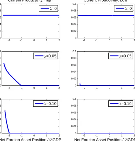
-2 -1 0 1 2 0 0.02 0.04 0.06 0.08 0.1
Current Productivity: High
D e fa u lt (t+ 1 ) / ∅ GDP λ=0 -2 -1 0 1 2 0 0.02 0.04 0.06 0.08 0.1
Current Productivity: Low λ=0 -2 -1 0 1 2 0 0.02 0.04 0.06 0.08 0.1 D e fa u lt (t+1 ) / ∅ GDP λ=0.05 -2 -1 0 1 2 0 0.02 0.04 0.06 0.08 0.1 λ=0.05 -2 -1 0 1 2 0 0.02 0.04 0.06 0.08 0.1
Net Foreign Asset Position /∅GDP
D e fa u lt (t+ 1 ) / ∅ GDP λ=0.10 -2 -1 0 1 2 0 0.02 0.04 0.06 0.08 0.1
Net Foreign Asset Position /∅GDP λ=0.10
Figure 1: Optimal Default Policies: The E¤ect of Default Costs
100% of GDP, see …gure 10 in Lane and Milesi-Ferretti (2007). Moreover, three out of the …ve industrialized countries approaching this boundary in the year 2004 later on faced …scal solvency problems (Greece, Portugal and Iceland). It thus appears plausible to assume that countries cannot sustain higher external debt levels without running the risk of a government default. Positive default costs and the small open economy assumption imply that the equilibrium outcomes are non-stationary, unless we choose1+r <1= . To insure that the equilibrium process is ergodic, we set the annual international interest rate …ve basis points below the rate implied by the inverse of the discount factor. Optimal default policies are rather robust to the precise number chosen.12
1 2
4.2 Evaluating the E¤ect of Default Costs
Figure 1 reports the optimal default policies for the next period as a function of the current (end-of period) net foreign asset position and the current pro-ductivity state.13 Each row in the …gure thereby corresponds to a di¤erent default cost parameterization ( ). To simplify the interpretation of results, the default policies and the net foreign asset positions are normalized by av-erage GDP. The panels on the left thereby depicts the optimal default policy in the high productivity state (zh) and the panels on the right policy for the low productivity state (zl). Appendix A.3 explains how the optimal policies can be determined numerically.
The graphs shown in the …rst row of …gure 1 report the outcome for the case when default costs are zero.14 Speci…cally, they depict the optimal amount of default in the next period, when the future productivity state hap-pens to be low (zl). Note that there will never be default if the productivity state zh realizes in the next period. Interestingly, the optimal amount of default is independent of the country’s net foreign asset position and almost independent of the current state of productivity.15 As is clear from proposition 1, these default policies fully insure future consumption against ‡uctuations in productivity.
The middle and bottom rows in …gure 1 report the optimal default policies when default costs equal 5% and 10% of the defaulted amount, respectively. For large parts of the state space default then ceases to be optimal. More-over, there is less default in the future if the current productivity state is low already. This is optimal because insurance against a future low state is more costly when current productivity state is low already, due to the persistence of productivity. Default continues to be optimal, however, if the net foreign asset position is su¢ ciently negative. Marginal utility of consumption is then very sensitive to further consumption ‡uctuations, because consumption ap-proaches its subsistence level as the net foreign asset position apap-proaches the limits implied by the (marginally binding) naturally borrowing limits.
Overall, …gure 1 shows that moderate levels of default costs shift optimal policy strongly towards using adjustments in international wealth to insure domestic consumption. Only if the country’s net foreign asset position ap-proaches the borrowing limit will a government debt default still be optimal. 5 Optimal Default and Economic Disasters
The previous section showed that with moderate levels of default costs it be-comes suboptimal to default on government debt, provided the country is not too close to its borrowing limit. In this section we evaluate whether this con-1 3As explained in section 2.3, the net foreign asset position is given by the optimal value
ofbin the corresponding period.
1 4Since there exists a multiplicity of optimal default policies when = 0, the …rst row
shows the outcome in the limiting case !0
1 5From equation (10) follows that the default in the next period does depend on the
clusion continues to be true for a setting with much larger economic shocks. This is motivated by the observation that countries occasionally experience very large negative shocks, as previously argued by Rietz (1988) and Barro (2006), and that such shocks tend to be associated with a government de-fault.16 To capture the possibility of large shocks, we augment the model by including disaster like shocks to aggregate productivity and then explore the quantitative implications of disaster risk on optimal government debt default decisions.
5.1 Calibrating Economic Disasters
To capture economic disasters we introduce two disaster sized productivity levels to our aggregate productivity process. We add two disaster states rather than a single one to capture the idea that the size of economic disasters is uncertain ex-ante. This will become important in section 6, when we dis-cuss how well simple …nancial instruments can approximate optimal default policies.
We calibrate the disaster shocks to match the mean and variance of GDP disasters, as documented in Barro and Jin (2011). Using a sample of 157 GDP disasters, they report a mean reduction in GDP of20:4%and a standard deviation of12:64%. Assuming that it is equally likely to enter both disaster states, this yields the productivity states zd = 0:9224 and zdd = 0:6696. Our vector of possible productivity realizations thus takes the form Z =
zh; zl; zd; zdd where the parameterization of the business cycle states zh; zl
is the same as in the previous section. The state transition matrix for the shock process is given by
= 0 B B @ 0:7770 0:1850 0:019 0:019 0:1850 0:7770 0:019 0:019 0:1429 0:1429 0:3571 0:3571 0:1429 0:1429 0:3571 0:3571 1 C C A;
The transition probability from the business cycle states into the disaster states is chosen so as to match the unconditional disaster probability of0:038, as reported in Barro and Jin (2011). We thereby assume that it is equally likely to reach both disaster states. The persistence of the disaster states is set to match the average duration of GDP disasters, which equals 3.5 years, see Barro and Jin. Finally, the transition probabilities of the business cycle states are adjusted to re‡ect the presence of disaster risk.
Since the presence of disaster risk strongly a¤ects the marginally binding NBLs (they become much tighter and potentially require even positive net foreign asset positions in all states), we recalibrate the subsistence level for consumptionc. As in section 4 before, we choose csuch that in an economy where bonds must be repaid always, the economy can sustain a maximum net
1 6
Barro (2006) and Gourio (2010) also allow for default on government bonds in disaster states. Since the focus of their analysis is di¤erent, they use exogenous probabilities and default rates.
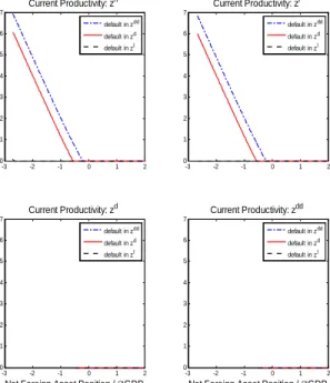
-10 -8 -6 -4 -2 0 2 0 0.2 0.4 0.6 0.8 1 Current Productivity: zh D e fa u lt(t+1 ) / ∅ GDP default in zdd default in zd default in zl -10 -8 -6 -4 -2 0 2 0 0.2 0.4 0.6 0.8 1 Current Productivity: zl default in zdd default in zd default in zl -10 -8 -6 -4 -2 0 2 0 0.2 0.4 0.6 0.8 1 Current Productivity: zd
Net Foreign Asset Position /∅GDP
D e fa u lt(t+1 ) / ∅ GDP default in zdd default in zd default in zl -10 -8 -6 -4 -2 0 2 0 0.2 0.4 0.6 0.8 1 Current Productivity: zdd
Net Foreign Asset Position /∅GDP
default in zdd
default in zd
default in zl
Figure 2: Optimal Default Policies with Disaster States ( = 0:1)
foreign asset of -100% of average GDP in the business cycle states (zh; zl).17 Choosing tighter limits does not a¤ect the shape of the optimal default policies but only shifts the policies reported in the next subsection ‘further to the right’.
5.2 Optimal Default with Disasters: Quantitative Analysis Figure 2 reports the optimal default policies for the economy with disaster shocks. Each panel in the …gure corresponds to a di¤erent productivity state today and reports the intended amount of default in tomorrow’s stateszl; zd
and zdd as a function of the country’s net foreign asset position today.18 We thereby assume that the dead weight costs of default equal 10% of the defaulted amount, corresponding to the default cost value used for computing the lowest row in …gure 1.
1 7
This yields an adjusted value ofc= 0:198.
1 8
Figure 2 shows that it is virtually never optimal to default in the low business cycle state (zl), unless the net foreign debt position is very close to its maximally sustainable level, similar to section 4 where we considered business cycle shocks only. Furthermore, for a wide range of net foreign asset positions, it is optimal to default if the economy makes a transition from a business cycle state to a disaster state, see the top panels in the …gure. Default is optimal for a transition to the severe disaster state (zdd), even when the country’s net foreign asset position is positive before the disaster. Overall, the optimal amount of default is increasing as the country’s net foreign asset position worsens. Yet, once the economy is in a disaster state, a further default in the event that the economy remains in the disaster state is optimal only if the net foreign asset position is very low, see the bottom panels of …gure 2. Since the likelihood of staying in a disaster state is quite high, choosing not to repay if the disaster persists would have very high e¤ects on interest rate costs ex-ante. As a result, serial default in case of a persistent disaster will not necessarily be part of the optimal default policy.
The overall shape of the optimal default policies is fairly robust to as-suming di¤erent values for the default costs . Larger costs shift the default policies towards the left, i.e., default occurs only for more negative net foreign asset positions. However, higher costs also tighten the maximally sustainable net foreign asset positions, thereby reducing the range of net foreign asset positions over which default occurs. Lower cost have the opposite e¤ect, i.e., they induce a rightward shift and allow to sustain more negative net foreign asset positions.
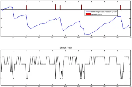
Figure 3 reports a typical sample path for the net foreign asset position and the amount of default implied by optimal policy for = 0:1. We start the path at a zero net foreign asset position and each model period corresponds to one year. The …gure shows that it is optimal to improve the net foreign asset position when the economy is in the business cycle states, with faster improvements in the high state. This is the case even though the international risk free rate is 5 basis points below the inverse of the domestic discount factor. A transition to a disaster state leads to a default provided the economy’s net foreign asset position is not too high (unlike in year 16). Also, following a disaster, the net foreign asset position deteriorates whenever the disaster persists for more than one period (see for example year 40), otherwise the net foreign asset position is largely una¤ected or improves even slightly (see year 85). Overall, the net foreign asset dynamics are characterized by rapid deteriorations during persistent disaster periods and gradual improvements during normal times.
6 Welfare Analysis and Approximate Implementation
This section determines the welfare e¤ects of letting the government choose whether or not to repay its debt compared to a situation where repayment is simply forced upon the government (or assumed) in each state. Furthermore, we study the approximate implementation of optimal default policies via a
20 40 60 80 100 120 140 160 180 200 -1.5 -1 -0.5 0 0.5
Default and Net Foreign Asset Position Path
Net Foreign Asset Position/∅GDP Default/∅GDP 20 40 60 80 100 120 140 160 180 200 z^dd z^d z^l z^h Time Shock Path
Figure 3: The Evolution of Net Foreign Assets and Default under Optimal Policy ( = 0:1)
combination of equity-like bonds and non-defaultable bonds. 6.1 Welfare Comparison
We now compare the welfare gains associated with optimal default policies to a setting in which repayment of bonds is required to occur in all states. We base our welfare comparison on the model with disaster states from section 5 and consider a broad range of default costs. We evaluate the utility consequences in terms of welfare equivalent consumption changes over the …rst 500 years. Speci…cally, lettingc1t denote the optimal state contingent consumption path in the no-default economy andc2
t the corresponding consumption path with
(costly) default, we report for each level of default costs the welfare equivalent consumption change! solving
E0 "500 X t=0 t((c1t(1 +!) c))1 1 # =E0 "500 X t=0 t(c2t c)1 1 #
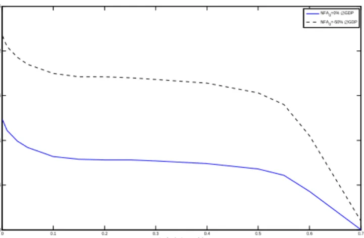
where the expectations are evaluated by averaging over 10000 sample paths. To highlight the e¤ects of the country’s initial international wealth position, we consider two scenarios, one where the initial net foreign asset position is zero and one where it equals -50% of average GDP.19 The outcome of this
1 9More precisely, we set the initial value of(1 )a
1+b 1 equal to these values and set
0 0.1 0.2 0.3 0.4 0.5 0.6 0.7 0 0.5 1 1.5 2 2.5 Default Costs (λ) W el far e Equi val ent Consum pt ion Gai n (i n % ) NFA0=0%∅GDP NFA0=-50%∅GDP
Figure 4: Welfare Gains from Using the Default Option
procedure is reported in …gure 4. It shows that the welfare gains amount to 1-2% of consumption each period for a broad range of default costs. The welfare gains are surprisingly robust to the level of the default costs, instead are more sensitive to the initial net foreign asset position. Yet, for default costs 0:5
the welfare gains from default decrease steeply. This has to do with the fact that for such high levels of the default costs it becomes suboptimal to insure against a future disaster state when the economy is already in a disaster, independently of the country’s net foreign asset position. This is shown in the lower panel of …gure 5 which reports the optimal default policies when
= 0:7. With these default costs, the government receives only 0.3 units of consumption for each unit of default. Since the likelihood of a speci…c disaster state (either zd or zdd) to re-occur is 0.3571, the cost of using the
default option for any of these states is0:3571=(1 +r)>0:3. Therefore, use of the default option is dominated by using the unconditional bond to transfer resources into a future disaster state. Repayment therefore optimally occurs in all future states, once the economy has hit a disaster state. As a result, the borrowing constraints tighten signi…cantly20 in the disaster states at this level of default costs and the required amount of insurance in the business cycle state (zl; zh) increases strongly as the net foreign asset position deteriorates.
6.2 Approximate Implementation
We now consider a setting where the government issues two kinds of …nancial instruments: a simple non-contingent bond that repays in all future contin-gencies, as well as an equity-like bond that repays one unit of consumption in normal times (zh; zl), but zero when a the disaster occurs (either zd orzdd).
2 0
-3 -2 -1 0 1 2 0 1 2 3 4 5 6 7 Current Productivity: zh D e fa u lt(t+1 ) / ∅ GDP default in zdd default in zd default in zl -3 -2 -1 0 1 2 0 1 2 3 4 5 6 7 Current Productivity: zl default in zdd default in zd default in zl -3 -2 -1 0 1 2 0 1 2 3 4 5 6 7 Current Productivity: zd
Net Foreign Asset Position /∅GDP
D e fa u lt(t+1 ) / ∅ GDP default in zdd default in zd default in zl -3 -2 -1 0 1 2 0 1 2 3 4 5 6 7 Current Productivity: zdd
Net Foreign Asset Position /∅GDP
default in zdd
default in zd
default in zl
Figure 5: Optimal Default Policy with Disaster States and High Default Cost ( = 0:7) -10 -8 -6 -4 -2 0 2 -1.2 -1 -0.8 -0.6 -0.4 -0.2 0 Current Productivity: zh Cont ingent Bond / ∅ GDP -10 -8 -6 -4 -2 0 2 -1.2 -1 -0.8 -0.6 -0.4 -0.2 0 Current Productivity: zl -10 -8 -6 -4 -2 0 2 -1.2 -1 -0.8 -0.6 -0.4 -0.2 0 Current Productivity: zd Cont ingent Bond / ∅ GDP
Net Foreign Asset Position /∅GDP
-10 -8 -6 -4 -2 0 2 -1.2 -1 -0.8 -0.6 -0.4 -0.2 0 Current Productivity: zdd
Net Foreign Asset Position /∅GDP
The fact that there is only one instrument but two disaster states implies that the government bond market is still far from complete, so that it is unclear to what extent the welfare gains from outright default could approximately be captured by this simple contingent bond structure. To make the setting with a contingent bond comparable to the setting with outright default analyzed in the previous section, we assume that the government must pay a cost per unit of equity bond issued in case a disaster state actually materializes. And to facilitate comparison to the results reported in section 5, we set = 0:1.
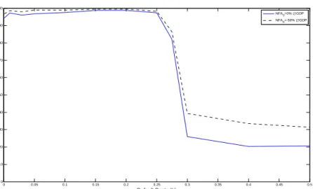
The optimal issuance of equity bonds is reported in …gure 6. The …gure shows that the equity bond policies are approximately a convex combination of the (negative of the) default policies for stateszdandzddshown in …gure 2. The …gure reveals that the government optimally issues the equity bond before an economic disaster actually happens and continues to issue such bonds while being in a disaster only if the net foreign asset position is su¢ ciently negative. Figure 7 reports how well the two available …nancial instruments allow to capture the welfare gains induced by optimal default policies, as reported in …gure 4. Speci…cally, the …gure depicts the share of the welfare increase that can be realized with the considered simple asset structure. It shows that for default cost up to about = 0:25 there is virtually no di¤erence between relying on optimal default policies or using the considered simple assets. This holds independently of the initial net foreign asset position. Yet, for su¢ ciently high levels of the simple asset structure cannot capture the achievable welfare gains from optimal default. Whenever 1 exceeds the combined persistence of the disaster states (zd and zdd), it becomes subop-timal to issue the equity bond if the economy is already in a disaster. As discussed in section 6.1, it is then optimal to issue non-defaultable bonds only. This tightens the (marginally binding) borrowing limits signi…cantly in the disaster states and decreases the opportunities for risk sharing, when compared to a setting with optimal default policies, where one can insure against disaster states individually.
7 Long Maturities and Optimal Bond Repurchase Programs We now discuss the e¤ects of introducing domestic bonds with longer matu-rity.21 Long bonds can o¤er an advantage over one period bonds, as considered in the previous part of the paper, if the market value of long bonds reacts to domestic conditions in a way that allows the government to insure against domestic shocks. It would be desirable, for example, if the market value of outstanding long bonds decreases following a disaster shock. This allows the government to repurchase the outstanding stock of debt at a lower price, thereby realizing a capital gain that lowers the overall debt burden. Unlike in Angeletos (2002), capital gains will not materialize unless the government plans not to repay fully the long bonds in (at least some contingency) in the future. The depreciation of the market value, thus, can only be induced via 2 1Introducing also longer maturities for the risk-free foreign debt has no consequences for
0 0.05 0.1 0.15 0.2 0.25 0.3 0.35 0.4 0.45 0.5 0 10 20 30 40 50 60 70 80 90 100 Default Costs (λ) W e lfa re G a in w ith E q u ity B o n d (re la tiv e to O p t. D e fa u lt in % ) NFA 0=0%∅GDP NFA 0=-50%∅GDP
Figure 7: Welfare Implications of Approximate Implementation
the anticipation of default in the future when long bonds mature.
Issuing long bonds will o¤er an advantage against outright default on ma-turing bonds, whenever the dead-weight costs associated with repurchasing bonds at a devaluated market price is lower than the dead weight costs of an outright default on maturing bonds today. If both costs are identical, i.e., if the capital gains on long bonds resulting from default in the future induce the same costs as a default on maturing bonds, then there will be of no addi-tional value associated with issuing long bonds. Yet, if the repurchase of long bonds at low prices fails to produce dead-weight costs, then the government could fully insure domestic consumption, i.e., achieve the …rst best allocation, independently of the costs associated with an outright default on maturing bonds. The optimal bond issuance strategy will then have the feature that the government issues each period long bonds that (partially) default at ma-turity, depending on the productivity realization tomorrow. The default at maturity needs to be calibrated such that the capital gains realized tomor-row fully insure domestic consumption against domestic productivity shocks, i.e., satis…es the proportionality restriction (10). Tomorrow, the government could then repurchase the existing stock of long bonds and issue a new long bonds with a new contingent repayment pro…le. In this way outright default on maturing bonds never occurs.
8 Conclusions
In a setting with incomplete government bond markets, debt default is part of the optimal government policy under commitment. The choice whether or not to repay maturing debt allows for increased international risk sharing and signi…cantly relaxes the net foreign debt positions that a country can sustain.
Moreover, it considerably increases welfare, even when default costs are siz-able. Default in low productivity states can be part of a country’s optimal policy in a setting with full commitment, especially if the net foreign asset position is close to the level implied by the country’s (marginally binding) natural borrowing limits.
A Appendix
A.1 First Order Equilibrium Conditions
This appendix derives the …rst order conditions for problem (5). We …rst rewrite the problem replacing beginning-of-period wealth by components (see de…nition (4)): max fbt;at 0;ekt 0;ect cg E0 1 X t=0 tu(ect) s:t: 8t:ect=ztekt 1+bt 1+ (1 )at 1(zt) e kt 1 1 +rbt pt at zt+1ekt +bt+ (1 )at(zt+1) N BL(zt+1) 8zt+1 2Z e w0=w0; z0 given;
Next, we formulate the Lagrangian and let t denote the multiplier on the budget constraint in period t, ztn the multiplier for the short-selling con-straint on the Arrow security that pays o¤ in statezn int+ 1, and !t+1 the
multiplier associated with the natural borrowing limits. We drop the inequal-ity constraints for ekt and ect, as the Inada conditions guarantee an interior solution for these variables. Di¤erentiating the Lagrangian with respect to the choice variables one obtains
e ct: u0(ect) t= 0 bt: t 1 1 +r + Et t+1+ Et!t+1 = 0 at(zn) : tpt(zn) + (znjzt) t+1(zn)(1 ) + ztn+ (znjzt)!t+1(zn)(1 ) = 0 8n2N e kt: t+ ekt 1 Et t+1zt+1+ ekt 1 Et!t+1zt+1= 0
Using the FOC for consumption to replace t in the last three FOCs, one obtains Euler equations for the bond holdings, the Arrow securities and capital investment: Bond: u0(ect) 1 1 +r + Etu 0(ec t+1) + Et!t+1 = 0 (11a) Arrow: u0(ect)pt(zn) + (znjzt)u0(ect+1(zn))(1 ) + ztn+ (znjzt)!t+1(zn)(1 ) = 0 8n2N (11b)
In addition, the Kuhn-Tucker FOCs include the following complementarity conditions: 0 at(zn) ? ztn 0 8n2N (11d) 0 znekt +bt+ (1 )az n t N BL(zn) ? !t+1(zn)) 0 8n2N:(11e)
Combined with the budget constraint, the Euler equations and the comple-mentarity conditions constitute the optimality conditions for problem (5). A.2 Proof of Proposition 1
We …rst show that the proposed consumption solution (8) satis…es the budget constraint, that the inequality constraints a 0 are not binding, and that the NBLs are also not binding. Thereafter, we show that the remaining …rst order conditions of problem (5), as derived in appendix A.1, also hold.
We start by showing that the portfolio implementing (8) in period t= 1
is consistent with the ‡ow budget constraint and a 0. The result for subsequent periods follows by induction. In period t = 1 with productivity state zn, beginning-of-period wealth under the optimal capital investment strategy (9) is
e
w1n zn(k (z0)) +b0+a0(zn) (12)
To insure that consumption can stay constant from t= 1 onwards we need again
c= (1 )( (zn) +we1n) (13)
for all possible productivity realizations n= 1; ::N. This provides N condi-tions that can be used to determine the N + 1 variables b0 and a0(zn) for
n= 1; :::; N. We also have the conditiona0(zn) 0for all nand by choosing
minna0(zn) = 0, we get one more condition that allows to pin down a unique
portfolio (b0; a0). Note that the inequality constraints on a do not bind for
the portfolio choice, as we have one degree of freedom, implying that the mul-tipliersvzn
1 in appendix A.1 are all zero. It remains to show that the portfolio
achieving (13) is feasible given the initial wealthwe0. Using (12) to substitute
e
w1n in equation (13) we get
c= (1 )( (zn) +zn(k (z0)) +b0+a0(zn))8n= 1; :::N:
Combining with (8) we get
(zn) +zn(k (z0)) +b0+a0(zn) = (z0) +we0
Multiplying the previous equation with (znjz0)and summing over all none
obtains E0[ (z1) +z1(k (z0)) ] +b0+ N X n=1 (znjz0)a0(zn) = (z0) +we0:
Using (z0) = k (z0) + E0[z1(k (zt+j)) ] + E0[ (z1)] and (3) the
pre-vious equation delivers
(1 )E0[ (z1) +z1(k (z0)) ] +b0+ (1 +r)p0a0= k (z0) +we0
Using = 1=(1 +r) this can be written as
(1 )E0[ (z1) +z1(k (z0)) ]
+1 p0a0+ (1 )b0+
1
1 +rb0+p0a0= k (z0) +we0 (14)
From (13) follows that the …rst terms in the previous equation are equal to
(1 )E0[ (z1) +z1(k (z0)) ] +
1
p0a0+ (1 )b0=c
so that (14) is just the budget equation for period zero. The portfolio giving rise to (13) int = 1 thus satis…es the budget constraint of period zero. The results fort 1 follow by induction.
It then follows from equation (13) thatwte is bounded, as (zt)is bounded, so that the process for beginning-of-period wealth does not involve explosive debt. The NBLs are thus not binding so that the multipliers!t+1 = 0 for all
tand all contingencies. Usingvzn
t 0,!t+1 0, the fact that capital investment is given by (9)
and that the Arrow security price is (3), the Euler conditions (11a) - (11c) then all hold when consumption is given by (8). This completes the proof. A.3 Numerical Solution Approach
To compute recursive equilibria for Problem 5 we apply a global solution method as to account for the non-linear default policies in our model. As endogenous state variable we use beginning-of-period wealth, de…ned as above. Combined with exogenous productivity shocks we de…ne our state space S to be
S = z1 N BL(z1); wmax ; :::; zN N BL(zN); wmax
where we set wmax such that in equilibrium optimal policies never imply
wealth values above this threshold. The NBLs are set such they are marginally binding. How these values are derived is shown in Appendix A.4.
We want to describe equilibrium in terms of time-invariant policy functions that map the current state into current policies. Hence, we want to compute policies
e
f : (zt; wt)!(fct; kt; bt; atg);
where their values (approximately) satisfy the equilibrium conditions derived above. We use a time iteration algorithm where equilibrium policy func-tions are approximated iteratively. In a time iteration procedure, one takes tomorrow’s policy (denoted by fnext) as given and solves for the optimal policy today (denoted by f) which in turn is used to update the guess for
tomorrow’s policy. Convergence is achieved once jjf fnextjj< and we set
e
f = f. In each time iteration step we solve for optimal policies on a su¢ -cient number of grid points distributed over the continuous part of the state space. Between grid points we use linear splines to interpolate tomorrow’s consumption policy. Following Garcia and Zangwill (1981), we can transform the complementarity conditions of our …rst order equilibrium conditions into equations. To solve for a root of the resulting non-linear equation system at a particular grid point we use Ziena’s Knitro, an optimization software that can be called from Matlab. For more details on the time iteration procedure and how one transforms complementarity conditions into equations, see for example, Brumm and Grill (2010). To come up with a starting guess for the consumption policy we use the fact that at the NBLs optimal consumption equals the subsistence level. We therefore guess a convex, monotonically in-creasing functiongwhich satis…esg(zi; N BL(zi)) =c8iand use a reasonable value forg(zi; wmax).
A.4 Natural Borrowing Limits (NBLs)
In this section we derive the NBLs that we use as lower bounds of the state space in our numerical application. For each state we de…ne the NBL as the maximum level of indebtedness that is still consistent with non-explosive debt. To put it di¤erently, we determine the minimum level of beginning-of-period wealth that is necessary to …nance the capital stock and portfolio (assuming consumption equal to the subsistence level) such that in all possible states tomorrow beginning-of-period wealth is at or above the respective limit. To compute these bounds we use Problem 5, simplifying the exhibition substan-tially and yielding the same solution as for Problem 2. To derive these state dependent borrowing limits we proceed as follows: we …rst postulate poten-tial solutions. Then we set up the problem that yields the minimum level of wealth today that can …nance a portfolio such that in all possible states tomorrow wealth is above the postulated solution. We use this problem for-mulation to derive the capital and portfolio decisions requiring the lowest level of wealth today and at the same time satisfy the wealth constraints in all states tomorrow. Using these optimal choices we can then set up the linear equation system to back out the minimum levels of wealth that can just be …nanced. To simplify exhibition we consider just two possible TFP shocks (N=2), denoted by z1 and z2. However, it is straightforward to extend our analysis to the general case of N TFP shocks, as we argue below. Note that we use only one Arrow security, the one for state 2. This choice is without loss of generality as with positive default cost costs will be minimized and there-fore the government will not acquire Arrow securities for the state where the least funds are needed. Without default costs, we can as well omit the Arrow security for the best productivity state as we have more assets than states available for trade. Finally note that we omit the short selling constraint on
the Arrow security to simplify the exhibition22. Step 1:
We denote potential solution byw1 and w2. Step 2:
For a given state s 2 f1;2g, we now want to determine the minimum level of wealth necessary to ensure that wealth tomorrow (w(s)tom)is above the
postulated bounds:
min w(s)
s:t: w(1)tom w1 w(2)tom w2
We can now use the budget constraint that is implied by consumption equal to the subsistence levelc: c=w(s) k q b pzs a;and use it to substitute
w(s)in the above minimization problem:
min
k;b;ac+k+q b+pz
s a;
s:t: z1k +b w1 z2k +b+ (1 )a w2
using w(1)tom=z1k +b and w(2)tom=z2k +b+ (1 )a.
The Lagrangian for this optimization problem has the following form:
L=c+k+q b+ps a+ 1(z1k +b w1) + 2(z2k +b+ (1 )a w2);
We can now derive …rst order conditions for all states. Solving these conditions for optimal choices in state 1 (state 2 is analogous) we get
k1opt= 1 (z2p 1 z1(p1 q)) 1 1 ; b1opt=w 1 z1(k1 opt) ; a1opt= w2 z2(kopt1 ) b1opt (1 ) : Step 3:
We now come back to the original …xed point problem: we want to determine the minimum values of wealth necessary to ensure that we are not below these values tomorrow. By setting the optimal choices derived above (which are a
2 2
When computing the NBLs in our numerical applications, it is important to take the short-selling constraints into account as with positive default costs they may actually be binding at the NBL
function of wealth) equal to the postulated wealth levels, the original …xed point problem translates into a linear equation system that yields in general a unique solution:
w1=c+k1opt+q b1opt+p1 a1opt w2=c+k2opt+q b2opt+p2 a2opt
Plugging in the optimal capital and portfolio choices derived above, we are left with an linear equation system containing only the wealth levels and exoge-nous parameters. The solution of the equation system yields the NBLs that we need for our numerical applications. For the general case of N TFP shocks, the analysis is conceptually equivalent, as the structure of the Lagrangian is preserved.
References
Adam, K. (2011): “Government Debt and Optimal Monetary and Fiscal
Policy,”European Economic Review, 55, 57–74.
Angeletos, G.-M. (2002): “Fiscal Policy with Noncontingent Debt and
the Optimal Maturity Structure,”Quarterly Journal of Economics, 117, 1105–1131.
Barro, R. (2006): “Rare Disasters and Asset Markets in the Twentieth
Century,”Quarterly Journal of Economics, 121, 823–866.
Barro, R. J., and T. Jin (2011): “On the Size Distribution of
Macroeco-nomic Disasters,”Econometrica (forthcoming).
Broner, F., A. Martin, and J. Ventura (2010): “Sovereign Risk and
Secondary Markets,”American Economic Review (forthcoming).
Brumm, J.,andM. Grill(2010): “Computing Equilibria in Dynamic
Mod-els with Occasionally Binding Constraints,”Mannheim University mimeo.
Buera, F., and J. P. Nicolini (2004): “Optimal Maturity of Government
Debt Without State Contingent Bonds,”Journal of Monetary Economics, 51(3), 531–554.
Eaton, J., and M. Gersovitz (1981): “Debt with Potential Repudiation:
Theoretical and Empirical Analysis,”Review of Economic Studies, 48, 289– 309.
Gourio, F.(2010): “Disaster Risk and Business Cycles,”Boston University
mimeo.
Grossman, H. I.,andJ. B. VanHuyck(1988): “Sovereign Debt as a
Con-tingent Claim: Excusable Default, Repudiation, and Reputation,” Ameri-can Economic Review, 78, 1088–1097.
Juessen, F., L. Linnemann, and A. Schabert (2010): “Understanding
Default Riks Premia on Public Debt,”TU Dortmund University Working Paper No. 27 SFB 823.
Lane, P. R., and G. M. Milesi-Ferretti(2007): “The External Wealth
of Nations Mark II: Revised and Extended Estimates of Foreign Assets and Liabilities, 1970-2004,”Journal of International Economics, 73, 223–250.
Marcet, A.,andA. Scott(2009): “De…cit and Debt Fluctuations and the Structure of Bond Markets,”Journal of Economic Theory, 144(2), 473–501.
Mendoza, E. G.,andV. Z. Yue(2008): “A Solution to the Disconnect
Be-tween Country Risk and Business Cycle Theories,”NBER Working Paper No. 13861.
Panizza, U., F. Sturzenegger,andJ. Zettelmeyer (2009): “The
Eco-nomics and Law of Sovereign Debt and Default,”Journal of Economic Literature, 47, 651–698.
Rietz, T. A. (1988): “The Equity Risk Premium a Solution,”Journal of
Monetary Economics, 22, 117–131.
Sims, C.(2001): “Fiscal Consequences for Mexico of Adopting the Dollar,”
Journal of Money, Credit and Banking, 33(2), 597–616.
Tauchen, G. (1986): “Finite State Markov-Chain Approximations to
Uni-variate and Vector Autoregressions,”Economics Letters, 20, 177–181.
Zangwill, W. J.,andC. B. Garcia(1981): Pathways to Solutions, Fixed