econ
stor
www.econstor.eu
Der Open-Access-Publikationsserver der ZBW – Leibniz-Informationszentrum Wirtschaft
The Open Access Publication Server of the ZBW – Leibniz Information Centre for Economics
Nutzungsbedingungen:
Die ZBW räumt Ihnen als Nutzerin/Nutzer das unentgeltliche, räumlich unbeschränkte und zeitlich auf die Dauer des Schutzrechts beschränkte einfache Recht ein, das ausgewählte Werk im Rahmen der unter
→ http://www.econstor.eu/dspace/Nutzungsbedingungen nachzulesenden vollständigen Nutzungsbedingungen zu vervielfältigen, mit denen die Nutzerin/der Nutzer sich durch die erste Nutzung einverstanden erklärt.
Terms of use:
The ZBW grants you, the user, the non-exclusive right to use the selected work free of charge, territorially unrestricted and within the time limit of the term of the property rights according to the terms specified at
→ http://www.econstor.eu/dspace/Nutzungsbedingungen By the first use of the selected work the user agrees and declares to comply with these terms of use.
zbw
Leibniz-Informationszentrum WirtschaftShonchoy, Abu
Conference Paper
What is Happening with the Government Expenditure
of Developing Countries - A Panel Data Study
Proceedings of the German Development Economics Conference, Hannover 2010, No. 2
Provided in cooperation with:
Verein für Socialpolitik
Suggested citation: Shonchoy, Abu (2010) : What is Happening with the Government Expenditure of Developing Countries - A Panel Data Study, Proceedings of the German
What is Happening with the Government
Expenditure of Developing Countries - A Panel
Data Study
∗Abu Shonchoy†.
The University of New South Wales January 21, 2010
Abstract
The paper focuses on the recent pattern of government expenditure for developing countries and estimates the determinants which may have influenced government expenditure. Using a panel data set for 111 developing countries from 1984 to 2004, this study finds evidence that political and institutional variables as well as governance variables significantly influence government expenditure. Among other results, the paper finds new evidence of Wagner’s law which states that peo-ples’ demand for service and willingness to pay is income-elastic hence the expansion of public economy is influenced by the greater economic affluence of a nation Cameron (1978). Corruption is found to be in-fluential in explaining the public expenditure of developing countries. On the contrary, size of the economy and linguistic fractionalization is found to have significant negative association over government expendi-ture. The study finds that military governments are more conservative in terms of large public expenditure other than spending on defence equipments.
Keywords: Government expenditure; Panel data; Corruption; Frac-tionalization; Governance.
JEL Classification: E01, E02, E61, E62, H2, H4, H5, H6, O11, O5.
∗
Acknowledgement : I am extremely thankful to Raghbendra Jha, Kevin J. Fox, Adrian Pagan and Denzil Fiebig for showing interest and giving me numerous ideas to fulfill this research. My heartfelt thanks goes to them. Usual disclaimers apply.
†
1
Introduction
After the second world war, governments even in the capitalist countries have become more influential as they provide social services, income supple-ments as well as produce foods, manage the economy and invest in capital (Cameron (1978)). In his seminal paper Aschauer (1989) found significant relationship between aggregate productivity and stock and flow of different government spending variables. He argued that non-military public capital is more important for productivity and also concluded that infrastructure spending (for example streets, highways, mass transit, sewer etc.) has the most rational for productivity. Aschauer’s conclusions were particularly im-portant for the developing countries where public capital symbolizes the “wheels” – if not the engine – of economic activity (WorldBank (1994)). Developing economics largely depends on government investments on health, education and public infrastructures to increase the economic growth, to im-prove social welfare and to reduce poverty. Many notable studies like Elias (1985), Fan et al. (2000, 2004) and Fan & Rao (2003) have contributed to the establishment of the positive linkage between government expenditure, production growth and poverty reduction. While these studies were con-cerned about the role of government on economic development, however, numerous studies have focused on the relationship between government ex-penditure and economic growth. Authors like Barro (1990), Devarajan et al. (1996), Bose et al. (2007) have found positive relationship whereas negligible or no relation between government expenditure and growth have been found by Landau (1983, 1985, 1986), Holtz-Eakin & Schwartz (1995), and Tanzi & Zee (1997). Hence,the relationship and causality between government expenditure and economic growth is quite ambiguous.
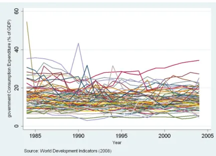
However, looking at the figure 1 where government expenditure of the de-veloping countries over the last three decades have been plotted, it is very surprising to see that the figure does not show any consistent trend at all. Whereas developed countries like United States, the share of GDP devoted to government expenditure has a steady and increasing trend since 1970 (Hy-man 1993, page 14). Thus, this rises the question of why the government expenditure of developing countries varies so much from countries to coun-tries? What are the factors and determinants that may have influenced the
government expenditure of the developing countries? Other than economic factors, is there any political, institutional or demographic factors which have influence over the government expenditure for developing countries? Only a handful of studies have been done on this literature since the major difficulties of such research is the paucity of data and the issue with data reliability which may have created impediment to these kind of research. The aim of this paper is to investigate the above mentioned research ques-tions with the aid of panel data. Using the panel data for the 111 devel-oping countries over the period from 1984-2004, this paper has estimated models to find the possible determinants of government expenditures. More-over, this study investigated the the influence on government expenditure by using categorized variables. The categories used in this paper are a) demographical variables b) fractionalization variables c) political variables and d) governance and institutional variables. Statistical evidence confirms that all these set of categorical variables have significant power in explaining the government expenditure in developing countries which is a noteworthy contribution to the literature.
2
Government Expenditure of Developing
Coun-tries
According to system of National accounting (SNA) 1993, Government Fi-nal Consumption Expenditure (GFCE) is the current expenditure by gen-eral government bodies on services (for example defence, education, public order, road maintenance, wages and salaries, office space and government-owned vehicles etc.) and net outlays on goods and services for current purpose. Exception has been made in the case defence expenditure, where purchase of durable military equipment (such as ships and aircrafts used for weapon platform) and outlays on construction works for military purposes. Consumption of fixed capital1 and intermediate consumption of goods and services (e.g. maintenance and repair of fixed assets used in production, pur-chases of office supplies and the services of consultants) are included whereas
1
According to SNA, consumption of fixed capital represents the reduction in the value of the fixed assets used in production during the accounting period resulting from physical deterioration, normal obsolescence or normal accidental damage.
the values of goods and services sold by government to other sectors are ex-cluded from such accounting. Transfer payments (e.g. interest payments for government debt securities and social assistance benefits) and subsidies are not included in this expenditure since the data is abstained from the national income accounts. As described in the ABS (Australian Beaureu of Statistics (2000), chapter 14 page 215, section 14.305) GFCE comprises the following
Compensation of employees paid to employee of general government bodies (other than producing capital goods)plus,
Intermediate consumption of goods and services (e.g. Purchases of office supplies and the services of consultants) less,
The value of goods and services sold by government to other sectors plus,
Consumption of fixed capital plus,
The timing adjustments for overseas purchases of defence equipment. Figure 1 shows the pattern of general government final consumption ex-penditure as a percentage of GDP for the 111 developing countries (using unbalanced data set) over the period 1994 to 2004. As we mentioned above, this figure is very interesting as it shows the nature of variability that exists with the pattern of GFCE as a percentage of GDP ratios for the developing economies. In the figure, one can easily observe that the ratios is jump-ing from 3% to even more than 50% with hardly any consistency or trends over the periods. If we use the same kind of diagrammatic analysis for the balanced data set then the figure remains the same.
[Figure 1 about here]
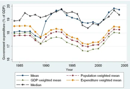
To understand the mean variation of government expenditures for devel-oping countries, we first plot the simple arithmetic mean of government expenditures (as a % of GDP) for over the year 1994 -2004 in figure 2. How-ever, such simple mean could be misleading since it does not account for the difference in number of countries as well as the difference in the size of economies, size of the population and the size of the actual government expenditure for different economies in each year. Hence, to accommodate these features, we constructed weighted arithmetic means. The weights we
used are population weight2, GDP weight3 and expenditure weight4. Also we have constructed the median government expenditures of these set of the countries to account for the center location of the variation of the expendi-ture over the years. It is interesting to observe that all the share weighted means and arithmetic mean follow almost the same upward trend. It is evi-dent from the figure that with the increasing share of population and GDP, developing countries increased their government expenditure. However, the median does not follow this trend at all. Surprisingly, quite oppositely, the median government expenditure over the years has a downward trend which may suggest that the countries which has larger share in total government expenditure has decreased their share of spending in relatively faster rates than from the other countries with low shares over the years.
[Figure 2 about here]
Now, if we compare the same set of mean and weighted means for the OECD countries for the comparable periods, we can see that there is hardly any trend in the weighted arithmetic means of government expenditures over the years though the arithmetic mean is showing an upward trend. In contrast of what we find in the median government expenditure in the developing countries, OECD countries show upward trend which could be due to fact that countries with higher government expenditure, actually increased their public expenditure share over the years.
[Figure 3 about here]
In figure 4, we have created different mean values of per capita income for the developing countries for the unbalanced data set. All the measures have shown consistent upward trends in the measure of per capita income which is a proxy for welfare and economic wellbeing. Therefore, from the diagram, it is distinct that these countries are improving over the years in terms of per capita income and welfare in aggregate level. Similarly, we plot the different mean values of government expenditures for the OECD countries of the comparable periods and find a strong upward trend in the per capita
2 Populationi/ n P i=1 populationi 3 GDPi/ n P i=1 GDPi 4GFCE i/ n P i=1 GFCEi
income.
[Figure 4 and figure 5 is about here]
It is compelling to observe that, on different average scales, the GFCE (as a % of GDP) fluctuate from little less than 17% to almost close to 20% for the OECD countries over the year 1994-2004. Whereas, using the same measuring tools, the fluctuation is from little over 10% to close to 15% for the developing countries which show that on an average developing countries government expenditure (as a % of GDP) is lower than OECD countries. Also, from the median analysis, it is noticeable that countries with larger share of government expenditure (as a % of GDP) have been reducing the share of their public expenditure whereas the trend is quite opposite in the case of OECD countries. Such observation is quite puzzling as it has been argued in the literature that due to the lack of large private sector, govern-ment expenditure actually plays a crucial role for any developing countries to have economic development, improvement in welfare, reduction in poverty and promotion of economics growth.
To understand what is happening with government expenditure for the de-veloping countries, we have to know what influences the government expen-diture and in what magnitude? The best approach to deal with this kind of research will be with the help of panel data which is a common practice in economic growth literature, as significant amount of analysis of growth have been done with panel data estimations. But the problem is the paucity of the data and the correlation between the explanatory variables which is very heard to deal with.
To the best of the authors knowledge, only a handful of works have been done on this literature. One of the earlier work is done by De Haan et al. (1996) which was done based on panel data of OECD countries for 12 years. In that paper, the authors concluded that investment spending of governments severely influenced by political decisions hence myopic government will re-duce the government spending more than governments with longer policy horizon. They have also concluded that private investments complements government investments spending. On the other hand, Sturm (2001) in his paper looked at the determinant of public capital spending for less develop-ing countries usdevelop-ing panel data. Sturm found “Political-Institutional”
vari-ables (like ideology, political cohesion, political stability, political business cycles, etc.) may not significantly influence the government capital spend-ing. However, instead of coming up with a model, he used Sala-I-Martin (1997) extreme bound approach to test various hypothesis which may have influence over public capital spending. Such approach has been criticized for omitted variable bias, multi-collinearity and data mining problem (Hendry & Krolzig (2004)). Hence, the conclusion drawn from the analysis could be misleading and questionable. Shelton (2007) tested several leading hypoth-esis of government expenditure using data from Global Financial Statistics data of IMF and other various sources. He has tested both separate sectors of government expenditure and different levels of government. He concluded that “preference heterogeneity leads to decentralization rather than outright
decreases in expenditure”. The method used in this analysis is random effect
model with strong assumption of cross sectional independence which is quite unusual for cross-country analysis. Hence the conclusion drawn in his paper could be misleading. Shelton used two demographic variables, percentage of population under 15 years and over 65 years, in the same regression which is known to have significant negative correlation. Furthermore, he used open-ness variable, which is endogenous in nature, as independent variable to explain contemporaneous government expenditures which made his analysis questionable. Other noticeable work is determinants of public expenditure is done by Fan & Rao (2003). In that paper, they found that much discussed structural adjustment programs by International Monetary Fund (IMF) has increased the spending of the government but all sector did not receive equal treatment. Further to their study, they got evidence of declining government spending for the agriculture, education and infrastructure in Africa. Gov-ernment spending on Agriculture and health sectors in Asia and education and infrastructure in Latin America have also declined due to such policy.
3
Literature Review
3.1 Income
One of the earliest and probably most frequently mentioned determinants of public spending is the economic growth which is famously known as
Wag-ner’s “law”. WagWag-ner’s “law of expanding state activity” ( Wagner 1883, pp.1-8) has been elaborated by many scholars of Public Economics (for ex-ample Bird (1971), Musgrave (1969) and Gupta (1968)). The law argues that peoples’ demand for service and willingness to pay is income-elastic hence the expansion of public economy is influenced by the greater eco-nomic affluence of a nation (Cameron (1978)). In other words, the scope of government tends to improve with the greater level of income and often said to imply that the income elasticity of demand for government is larger than unity (Flster & Henrekson (2001)).
Several scholars have rejected Wagner’s argument and find evidence against it like Bird (1971), Musgrave (1969) and Gupta (1968). Peacock & Wiseman (1967) even rejected the “historical determinism” argument of Wagner’s law. Wildavsky (1975), on the other hand, provided a reverse argument which has been termed as “counter-Wagner” law by Cameron (1978). Wildavsky’s argument would predict a negative relationship between growth and gov-ernment expenditure, indicating greater expansion of public expenditure for low-growth countries. Cross-country studies like Wagner & Weber (1977), Abizadeh & Gray (1985), Ram (1987), Easterly & Rebelo (1994) and Shel-ton (2007) did not found one cohesive conclusion regarding Wagner’s Law. Interestingly, all of these aforementioned studies have studied the correla-tion of par capita income and the size of government to get the evidence in favor of Wagner’s Law. However, Henrekson (1993) remarked that major-ity of the work in support of Wagner’s law have been done in levels hence could be spurious if there exist cointegrated relationship between these two variables as suggested in Granger & Newbold (2001). In our present study we would like to test for Wagner’s law and its relationship with government expenditure by using per capita income and the growth of per capita income as regressors for GFCE as a percentage of GDP.
3.2 Openness
Among others, Cameron (1978) was the most influential in establishing a robust relationship between trade openness and government expenditure. Using the sample of 18 OECD countries, he found evidence of countries having large expenditure increase with more trade openness from the
pe-riod of 1960 and 1975. He argued that more open economies will have higher rates of industrial concentration, lead to more unionized labor mar-kets which, through collective bargaining, influence the public spending for social protection and social infrastructure. Improving on Cameron’s work, which was limited to 18 wealth rich countries, Rodrik (1998) demonstrated a significant positive correlation between openness and government size us-ing 100 plus country sample. Rodrik argued that Cameron’s explanation of collective bargaining and labor unionization is somewhat unlikely to explain the relationship since the labor organizations are not well organized hence less influential in developing countries. Rodrik explained such correlation between openness and government expenditure as social insurance against external risk. More open economies are exposed with greater external risk such as exchange rate fluctuation, supply or demand variability in the world market. Governments mitigate such exposure to risk through increasing“the
share of domestic output they consum”. For developed country, with proper
administrative capacity, such risk is mitigated through spending on social protection while in developing countries, lacking the administrative capacity, mitigate such risk through simpler solution like public employment, in-kind transfers or public work programs. Other than these two major studies, scholars like Schmidt (1983), Saunders & Klau (1985) also have found a correlation between trade openness and the size of the public sector. Hence a positive correlation between openness and GFCE as a percentage of GDP has been hypothesized.
3.3 Aid
Foreign aid as an institution began in 1947 and by 1960 it expanded across many developing countries in Asia and Africa. Advocates of aid argue that aid helps developing countries to release binding revenue constraints, strengthening domestic institution, pay better salaries to public employees, help in poverty-reducing spending and improve the efficiency and effective-ness of governance (Brautigam & Knack (2004)). On the contrary, higher aid inflows could promote rent-seeking behavior by domestic vested interests that outcry for tax exemptions or seek to avoid paying taxes which leads the revenue to decline (Clements et al. (2004)). Also, critics argued that aid could lead to increased public and private consumption rather than
invest-ment, and could have contributed less to growth (Please (1967); Papanek (1973); Weisskopf (1972)). In his classic paper Heller (1975) showed that aid increases investment and simultaneously reduces domestic borrowing and taxes which eventually influence on public consumption. But the mag-nitude of such influence over public consumption depends on the type of aid as grants have strong “pro-consumption” bias whereas loans are more “
pro-investment”. Improving on Heller, Khan & Hoshino (1992) concluded that
aid generally increase government consumption and the marginal propen-sity to consume out of foreign aid is less than one, which means some public investment is also financed out of aid. Moreover, many researchers (Otim (1996); Ouattara (2006); Remmer (2004)) have found considerable linkage between aid and expansion of government spending. Since recent initia-tive have called for shifting aid more towards grant, believing that excessive lending has led to huge debt accumulation in many countries and did not contributed to reach their development objectives (Clements et al. (2004)). Therefore, a positive relationship between aid and GFCE as a percentage of GDP has been hypothesized.
3.4 Debt
Due to the rising interest rates, price hike of oil imports and unfavorable con-ditions for primary export product, government revenues has been declining for many developing countries since 1979. During that era, expanded invest-ment programs were financed with foreign debt for many countries. These fiscal deficits further raise the external public debt through the channels of public borrowing. External borrowing usually encourages fiscal over-spending which raises the government expenditure. Similarly, the public debt burden may directly impact the government expenditure since an in-crease in the burden of the debt beyond a specific threshold level could gen-erate disincentives for the public sector and investment or productive and adjustment efforts which is known as “debt-overhang” hypothesis (Krugman (1988)). Also, over-valuation of the official exchange rates has encouraged capital flight driven external borrowing for these nations (Mahdavi (2004)).5
5See Ndikumana & Boyce (2003) for a discussion of the interaction between capital
However, 1980s “debt crisis” has enforced highly indebted countries to re-duce fiscal deficit and adjust expenditures since access to foreign capital mar-ket became very constrained. Also, International Monetary Fund’s (IMF) macroeconomic adjustment program compelled many indebted countries to reduce fiscal deficit as part of the condition for their debt restructuring and relief initiative. Efforts intended to reduce fiscal deficit have distribution issues between expending reduction and revenues increment. In general, the spending side of the budget is likely to bear a heavier toll of the deficit lessen-ing than the revenue sides as spendlessen-ing cuts are more quickly applicable than generating higher revenue through taxation. Since, interest payments on the debt is relatively inflexible and significant component of the public expendi-ture, expenditure cuts may fall upon current income and consumption levels of population which will lead to adverse welfare impact. In the case of de-veloping countries, expenditures that directly benefit the low-income groups of the population (such as education, medical, social safety net programs) should be protected to reduce the social cost of these adjustments (Cornia et al. (1987)). Hicks & Kubisch (1984) and Hicks (1989) has found that unlike capital spending, social and defense spending seemed to be protected whereas capital intensive sectors like infrastructure and wages and salaries of public employees carry the major burden of expenditure reduction. Mah-davi (2004), in contrast, found that the share of politically sensitive category of wages and salaries of public employees might not adversely affected by the debt burden. Hence, the impact of debt on GFCE will be an interesting outcome in this study.
3.5 Fractionalization
Many researchers have argued that cross country difference in public pol-icy, government expenditures and other economic factors could be explained better by investigating the ethnic diversity among countries. The main ra-tionale for such argument is that economy with higher ethnic fragmented population may find it difficult to agree on public expenditures and effective policies which may lead to political instability. Also, polarized ethnic society weakens the centralized control of government (Shleifer & Vishny (1993)), deteriorates the check and balance (Persson et al. (1997)) and encourages the rent seeking behavior (Mauro (1995)). Easterly & Levine (1997) find a
strong negative relationship between ethnic fragmentation and some public goods (like telecommunication, transportation electricity grids and educa-tion) in African countries. They concluded that, due to such high degree of ethnic divisions and conflicts, African countries largely adopted “growth-retarding” policies over the years which could be one of the principle rea-sons of Africa’s recent growth tragedy. As a result of their paper, ethnic fragmentation became a standard control for the analysis of cross-country regressions (Alesina et al. (2003). Alesina et al. (1999) in their classic paper showed that shares of spending on productive public goods like education and transportation is inversely related with city’s ethnic fragmentation. Us-ing the data of U.S. they concluded that preference of public policy is corre-lated with ethnicity therefore ethnic conflict is an important determinant of public finance. As a result, ethnic polarization and interest groups politics would encourage “patronage” spending and discourage non-excludable pub-lic goods. However, the effect of ethnic polarization on total government expenditure is ambiguous because of the reverse effect of aforementioned difference in the spending pattern of the government. In a follow-up paper, Alesina et al. (2000) further demonstrated using US data that more ethni-cal fragmentation leads to bigger public employment since governments of ethnically diverse economy tends to use public employment as an “implicit subsidy” to ethnical interest groups who would otherwise receive transfer. Politicians are interested in such strategy to disguise their redistributive policies to avoid opposition of precise tax-transfer schemes. While all the research mentioned above used indices based on “ethnolinguistic fractional-ization (ETF)”, which relies mainly on linguistic heterogeneity other than racial or skin color distinctions.
Alesina et al. (2003) came up with a new measure of ethnic fragmentation based on a broader classification of groups. Their study took account of racial, language as well as religious characteristics within a country using different sources. The data set provides measure for many more countries than those of ETF. This new data set has three different indices of ethnicity, language and religion for each country. The authors find that ethnicity, language and religion lead to different results when they are entered to explain government quality especially the quality of institutions and policies. So, following the recent trend in cross-country regressions, we also look at
the effect of ethnic, language and religious fractionalization on the GFCE as a percentage of GDP.
3.6 Size of the Economy
An inverse relationship between government size and country size could arise from economics of scale in the provision of public goods (Shadbegian (1999, 1996); Owings & Borck (2000); Bradbury & Crain (2002); Remmer (2004)). Recent studies on the literature of country formation, like Alesina & Spolaore (1997) and Alesina & Perotti (1997) also suggested that country size and government size are interconnected. Alesina & Wacziarg (1998) provided an explanation for their findings of negative relationship between country size and government consumption. They argued that expenditure related to non-rival public expenditures such as roads, parks and general administrations, when shared over large population lowers the per capita costs for a given level of provision. Moreover, larger population lead to increased hetero-geneity of preferences over the provision of public goods which could lower the per capita expenditure on public outlays. The equation developed by Dao (1994) on per capita expenditure on government services shows a direct relationship between population and per capita expenditure. Dao (1995), however, showed that the effect of population on government expenditure is non-linear since he found ambiguous relationship between disaggregate government expenditures with population. Sanz & Velzquez (2002) showed significant negative relationship on sector specific government expenditures and population specially in the case of pure public goods.
3.7 Demographic Pattern
Since government spending specially health care and social security tends to be related with the demographic structure of any economy, we need to take into account the variations of dependency ratio of the population (Sanz & Velzquez (2002), Remmer (2004)). The dependency ratio is measured as the percentage of population that is 65 years of age or older. Similarly, high degree of urbanization leads to greater demand for services like education, roads and transportation. Hence, greater urbanization will influence more
government expenditure spending on infrastructure and public utilities.
4
Data and Hypothesis
4.1 Hypothesis
Interestingly, numerous hypothesis has been proposed in various literature about the determinant of the Government expenditure. Unfortunately, there is no comprehensible theory and different studies are quiet independent and fragmented. The approach taken by this paper is to test a number of dif-ferent hypothesis which has been used and proposed in various literature. Sometime, the hypothesis may be conflicting in nature but at least this will give us some idea about the determinants of government expenditure pattern of developing countries.
One method cross country panel studies typically use is converting the data from level to some reference percentage since bigger economy tends to have bigger economic variables if we capture the variable in levels. But, rather than levels, we are particularly interested in percentage allocation of eco-nomic variables with respect to GDP. Similarly, for the demographic vari-ables we converted all the varivari-ables as a percentage of total population. To capture the size of the country, we used the log of population to have a better fit. Fractionalization variables are expressed in probability whereas most of the political variables are expressed as dummy variables. The rest of the variables are expressed as index.
Hypothesis used in this paper can be categorized to the following sets of explanatory variables:
Base variables: Aid per capita, Total debt (in % of GDP), Openness (in % of GDP), GDP per capita and Log of population.
Demographical variables: Elderly population, ages 65 and above (% of total population), Young population, ages 15 and below (% of total popula-tion), Urban population (% of total) and Population growth rate (annual).
Fractionalization variables: Ethnic fractionalization, Linguistic fraction-alization and Religious fractionfraction-alization.
Political institutional variables: Years of office (number of years the chief executive of the nation is in the office), Number of government seats, Number of opposition seats, Military officer (1 if the chief executive a mil-itary officer), Legislative election (1 if yes), Executive election (1 if yes), Nationalist party (1 if yes) Regional party (1 if yes) and polity index (varies from -10 to +10).
Governance variables: Voice and accountability (varies from -2.5 to +2.5), Political stability and absence of violence (varies from -2.5 to +2.5), Control of corruption (varies from -2.5 to +2.5), Government effectiveness (varies from -2.5 to +2.5), Regulatory quality (varies from -2.5 to +2.5) Rule of law (varies from -2.5 to +2.5) and Corruption perception index, CPI (varies from 0 to 145).
Detail description of these variables could be found at table 12.
4.2 Data Issues
All the base variables and the demographical variables have been taken from the World Bank Development Indicators CD-ROM 2008 (WDI 2008) pub-lished by the World Bank. The Fractionalization data has been taken from Alesina et al. (2003). In this paper, new measures of ethnic, linguistic and religious fractionalization for about 190 countries have been constructed. However, due to high degree of multi-colinierity in our models we could not able to use more than one fractionalization variable at a time. The set of political variables has been taken from Database of Political Institu-tions (DPI2004) provided by the Development Research Group of the World Bank. This data set is constructed by Beck et. al. (2001) and the index created in this series has been described in their appendix. In the case of Institutional variables, the data was not available for the period 1997, 1999 and 2001. For this set of variables, we have constructed the value of the missing year by using the mean of the corresponding forward and backward year. Except for the CPI data, the Institutional variables have been taken from the Worldwide Governance Indicators (WGI) project by the World Bank. This data set is constructed by Kaufmann et al. (2005) which is only available from 1996- 2005 period. The CPI index has been taken from the Transparency International’s web cite. The “Polity Score” is a standard
measure of governance on a 21-point scale ranging from -10 (dictatorial) to +10 (consolidated democracy).
5
Methodology
Various literatures of time-series-cross-section data analysis have used both country specific fixed effect model as well as random effect models. Initially we have tested for the poolability estimation and the result suggest that there exists significant individual country effect implying that pooled OLS would be inappropriate. Then we have tested with the basic specification for the Hausman specification test (Hausman (1978)) which could not reject the null hypothesis that random effect model is inconsistent, hence we could use the random effect model which is also persistent with the work of Shelton (2007).
The problem with random effect estimation is the strong assumption about cross-sectional independence across panels. Such assumption of independent error terms across panels is very rare to find in cross country studies. In particular, as stated in Beck (2001) the errors of time-series-cross-section models may have (a) panel level heteroscedasticity which means each coun-try could have its own error variance i.e. E(i,tj,s) =σi2 ifi=j and s=t or 0 otherwise; (b) contemporaneous correlation of the errors which means error for one country may be correlated with the errors of the other countries in the same year i.e. E(i,tj,s) =σi,j if i 6=j and s =t or 0 otherwise or (c) serial correlation which means errors for a given country are correlated with previous errors for that country i.e. i,t = ρi,t−1 +vi,t. Hence, we would expect to observe panel heteroscedasticity, contemporaneous correla-tion and serial correlacorrela-tion in the error term of the time-series-cross-country regressions as error variance varies from nation to nation.
To test the hypothesis of cross-sectional independence in panel-data models with small T and large N we could use semi-parametric tests proposed by Friedman (1937) and Frees (1995, 2004) as well as the parametric testing procedure proposed by Pesaran (2004).6 In our study we found evidence
6
I usedxtcsd routine in STATA which is developed by De Hoyos & Sarafidis (2006) to check such assumptions in STATA.
of contemporaneous correlation across the units using the above mentioned tests. Also we tested for the group-wise heteroscedasticity and autocorrela-tion in the panel data with the help of modified Wald test and Wooldridge test respectively. Both of the test showed evidence of heteroscedasticity and autocorrelation in the data set. As mentioned by Baltagi (2005, pp 84) as-suming homoscedasticity disturbances and ignoring serial correlation when heteroscedasticity and serial correlation are present will result consistent but inefficient estimation and standard errors could be wrong. As a result, models needed to be corrected for such patterns of the error term to get consistent and efficient estimates of the regressors.
Two standard methods used by the researchers to correct such problems in the data, which are Feasible Generalized Least Square (FGLS) method and Prais-Winsten transformation procedure. Both estimates will produce consistent estimates as long as the conditional mean is correctly specified. In our study we choose to use FGLS procedure for its power to produce estimates with time invariant variables. Under FGLS, Beck & Katz (1995) has suggested to use panel specific AR1 parameters over single AR parame-ters in case of time-series-cross-sectional models. Nonetheless, the quality of national data of the developing countries, which we are using for the study, varies significantly among countries which could also be a potential source for the heteroscedastic error structure in the model.
It is argued that current political, social and economical institutions for many countries are largely determined ages ago by their past history, geog-raphy, religion and climate. etc (Putman (1993) and Acemoglu et al. (2001)). To capture such time independent constant effect, we used continental dum-mies. All the regression estimations have year specific dummies which have accommodated the year specific variation in the model. We tested for panel unit root process in the dependent variable for both common and individual unit root process and five out of six tests rejected the null of having a unit root process in the dependent variable. Government expenditure responses are likely to occur with a delay, hence to capture such phenomenon as well as to tackle the endogenous nature of the economic variables one year lagged variables have been used. Such lag independent variables in the estimations will control for any two way causality between dependent and independent variables.
In order to test the robustness of the model, we have tried to impute some missing variables of the countries to improve the degrees of freedom of the model and also to check the persistence of the estimations. There are some countries which have very good data but has only one or two years missing data for some variables. We have used linear trend imputation techniques to estimate the missing values for this countries.7
The basic specification for the model is
GFCEi,t =α+β∗Base Variablesi,t+γ∗Yeart+δ∗Continent Dummyi+i,t. Where i denoted for the country and t denoted for the year. For an ex-tended specification we will keep the basic specification with added set of new variables.
6
Estimation results
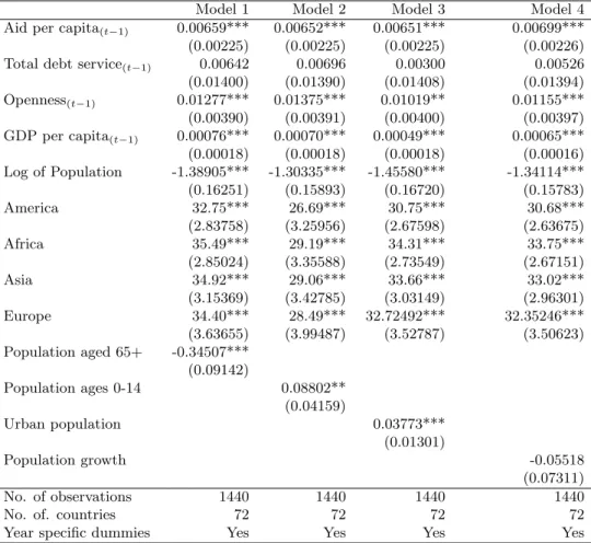
6.1 Basic Specifications
Table 1, reports the basic specifications using both balanced and unbalanced data set and the results are consistent in both regressions. Other than the coefficient of the total debt services, all other variables are highly statisti-cally significant. Such results shows evidence that public debt burden may not directly impact on government spending immediately. Another explana-tion could be that instead of cutting the government expenditure to finance debt burden, developing countries tend to generate higher revenue through taxation since raising revenue is quicker than cutting the pre-planned gov-ernment expenditures. The point estimates from table 1 suggests that one standard deviation increase in income per capita (1543) in the last year will increase the GFCE of the current year by almost 1.31% of GDP by using unbalanced data set (0.96% of GDP in case of balanced data set) suggest-ing the evidence in favor of the Wagner’s Law. This result recommends
7
The maximum number of imputation done for any country for any variable is two years. If the data is missing more than two years, we have dropped the country. Imputation has been done only for the voice and accountability, political stability and control of corruption variables.
that with the increase in the per capita income of the population, devel-oping economies tend to expand their public spending due to the emerging pressure on the demand of publicly available goods and services.
[Table 1 about here]
The results in table 1 explores that there exist a strong association between past years’ trade openness and current government expenditure for the de-veloping countries which confirms the results of Cameron (1978), Rodrik (1998) and Shelton (2007). The association between exposure to external risk trough trade openness increases the government expenditure since gov-ernments need to provide more resources for the people to mitigate the external shocks which may occur in the world economy. This extra expen-diture could be used for social security and welfare spending purpose or could be directed towards creating more jobs through larger public work programs. Moreover, greater trade openness leads to greater demand for transport facilities, institutes, administrative supports and infrastructures which could also lead to bigger expenditures for the governments.
Table 1 also revealed the strong positive association between past years per capita aid with current government expenditure. The point estimates suggests that one standard deviation increase in per capita aid of the past year could lead to an increase in GFCE of 0.19% of GDP (using unbalanced data set). As mentioned in Clements et al. (2004), an increase in the financial aid could provide several choices for a government like reducing revenues, increasing expenditure, reducing the domestic borrowing or a combination of all the three options. The result in the regression shows the evidence that aid actually increase the government expenditure significantly for the developing countries. This finding is not surprising since financial assistance provided by the donors and international agencies is mostly in the from of non-fungible project assistance which requires matched spending from the recipient government.
Furthermore, we find that a one standard deviation increase in the log of population leads to a decrease in GFCE by 2.3 % of GDP. Such result shows evidence of large preference heterogeneity leaded reduction in government expenditure as hypothesized by Alesina & Wacziarg (1998). Among the continental dummies, we can observe that on an average, GFCE as a % of
GDP is higher in European countries than other continents which is quite consistent in other extended specifications as well. On the contrary, Latin American countries have relatively smaller share of GFCE as a % of GDP than other continents. This particular result conforms that European coun-tries tend to accommodate greater degree of publicly provided goods and services like social security and health care than other continents which has increased the relative size of their government expenditures.
6.2 Demographic Variables
Table 2 and 3 have the extended specifications of base variables with a set of demographic variables which will reveal the association of government expenditure with demographic variables. Comparing the base variables of table 1 with those of table 2 and 3 show the consistency across the estima-tions. Model 1 in table 2 and 3 show that, with a increasing fraction of the population over 65, developing countries tend to have smaller government expenditure as a % of GDP. The reason for such finding is two fold. Firstly, analyzing from the demand side, developing countries tend to have more younger population than richer countries hence their expenditure on senior citizens will be relatively smaller. Moreover, in most developing countries, it is very difficult to find an adequate and established pension and social se-curity system for the aging population. Also due to lack of resources, these governments mostly prioritize their expenditure towards revenue generat-ing sectors rather than spendgenerat-ing on older population. Hence, in developgenerat-ing countries, elders are mostly looked after by their immediate family members. Secondly, analyzing from the supply side, population aged over 65 contribute less to the economy which eventually reduce the revenue collected through taxation. As a result, with the growing fraction of the population aged over 65, governments will have less revenue and will have less allocation for the government expenditure as a share of GDP.
[Table 2 and 3 about here]
On the contrary, a strong and positive association has been found between the population aged less than 15 and government expenditure as a percent-age of GDP and such finding is consistent even in the balanced panel. This result reveals that developing countries on an average allocate more
expen-diture with the growing fraction of younger population. A one standard de-viation increase in the fraction of population less than 15 is associated with an increase of GFCE by 0.66% of GDP. Such rise in expenditure mostly directed towards the education and health sector of the economy to fulfil the emerging demand for these services with the greater fraction of young population. Similarly, strong positive association between degree of urban-ization and public expenditure has also been found in both balanced and unbalanced data set showing the emerging demand for public utilities and services in the urban areas as the fraction of population living in the urban areas increases. Internal rural to urban migration is a common phenomenon in the developing countries since the expected income in the urban areas is higher than the rural areas. As degree of urbanization increases, govern-ments need to spend more on transportation, public utilities and amenities to fulfil the rising demand for such services.
However, no significant correlation between government expenditure and population growth could be found in the regression which is quite a puzzling result. One of the recent policy developments in developing countries has been the population reduction program to restrict the population growth. As a result there exist very small variation for the population growth variables in the panel data set which could lead to such insignificant relationship between population growth and public expenditure.
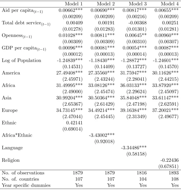
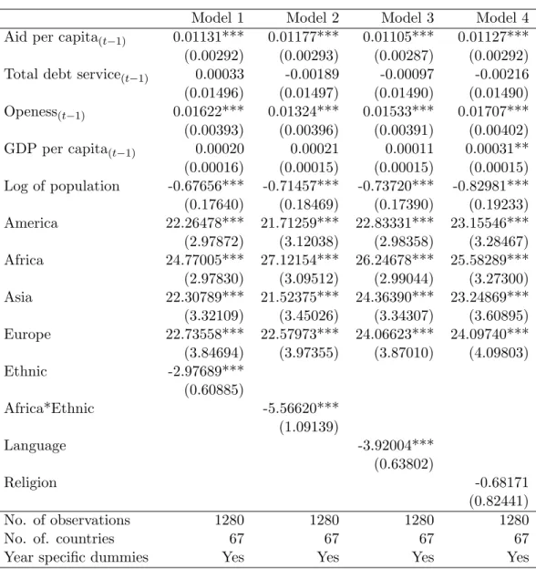
6.3 Fractionalization variables
Three different measure of fractionalization; ethnic, language and religion have been used with the base variables to test the association of fraction-alization with government expenditure. The results of such regressions are reported in table 4 and 5 by using both balanced and unbalanced data set. Both the table 4 and 5 show that base variables are showing consistency with appropriate signs and significance level. The coefficient of ethnic fractional-ization shows no significant power in explaining the variation in government expenditure in case of unbalanced data set whereas the variable is highly statistically significant in case of balanced data set. One possible explana-tion for such difference in estimaexplana-tion could be due to the loss of degrees of freedom in balanced data set. The data reveals that on an average ethnic
fractionalization is remarkably higher in the African nations than other con-tinents. To be specific, the average probability that two randomly selected people will not belong to the same ethnic group in African countries is 0.25 whereas the average is only 0.06 in European nations. In our data, eigh-teen out of twenty most ethnically heterogenous countries belong to Africa showing the degree of ethnic diversity exist in Africa. Therefore, in stead of using ethnicity in explaining the cross country difference in government expenditure, it would be more sensible and interesting in exploring the asso-ciation between ethnic diversity and GFCE in African nations. Model 2 in table 4 and 5 reveals that ethnic fractionalization is significantly negatively correlated with government expenditure and has a economically large coeffi-cient in both balanced and unbalanced data set. Ethnic diversity influences the economic performances of any nation and has direct influence over the growth performance (Easterly & Levine (1997)). The estimation confirms that with a greater degree of ethnic heterogeneity, nations belong to Africa tend to reduce the size of the government expenditure. High degree of eth-nic fractionalization lead to under provision of publicly available services like education, transportation and infrastructure which have negative im-pact on the economic growth of the continent and could be used to explain the recent growth tragedy of Africa.
[Table 4 and 5 about here]
Linguistic fractionalization, on the other hand, is more or less a common phenomenon in any continent and has significant explanatory power to ad-dress the variation of government expenditure in cross country regression. Linguistic fractionalization could be quite high in countries where ethnic fractionalization is not that extreme. For example, India where the eth-nic fractionalization is 0.41 though linguistic fractionalization is almost 0.81 which is quite extreme. Furthermore, linguistic heterogeneity is intense even in Latin American countries along with Asia and Africa. Regression on un-balanced data reports that a one standard deviation increase in linguistic fractionalization is associated with an decrease of GFCE by 1.07% of GDP. However, religious fractionalization does not seem to be correlated with government expenditures. The difference in the result between religious and other heterogeneity is quite suggestive since religious fractionalization mostly endogenous in nature (Alesina et al. (2003)). Individuals and families
can convert to other religion quite easily. Also a high degree of religious het-erogeneity could be sign of tolerance and harmony rather than conflict which could also explain the reason for not getting any statistical significance of religious fractionalization and government expenditure. Our results broadly remain the same even when we used the extended specification to under-stand the role of fractionalization in explaining the government expenditure (see table 10).
6.4 Political institutional variables
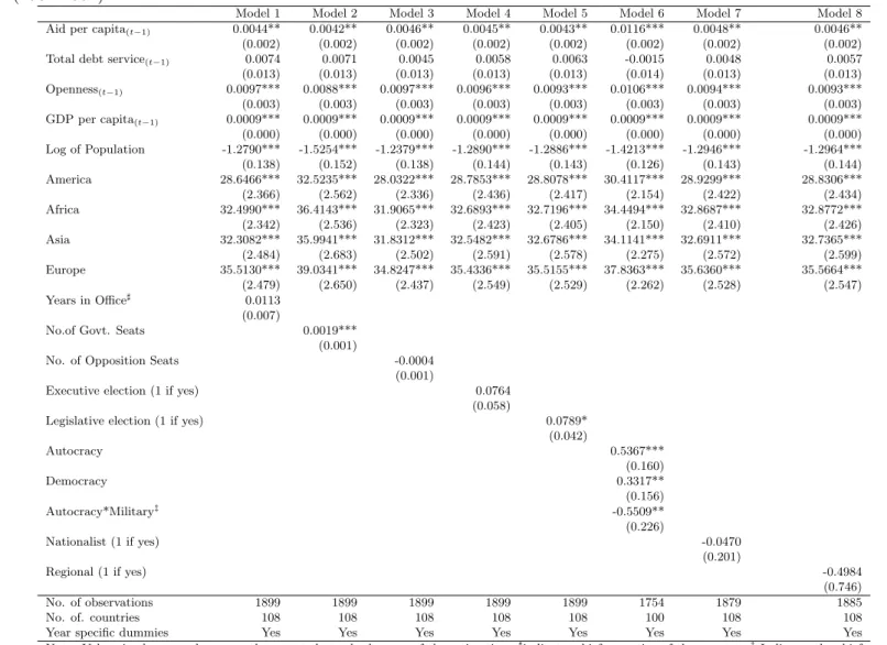
Political institutions play pivotal role in deciding the shape and the size of the government. Hence, we need to understand the determinants of gov-ernment expenditure through the lens of political institutions. However, inadequate data on political institutions of countries especially for devel-oping countries has made cross-country empirical work handicapped. We used a recent data set, the Database of Political Institutes (DPI), which is developed by Development Research Group at the World Bank. DPI contains numbers of variables for the period we are interested in and have many dimensions to have better understanding of the political economy on government expenditure.
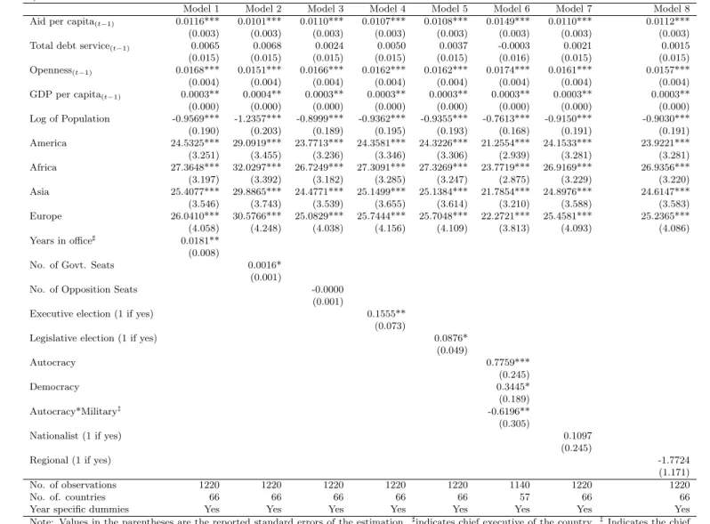
One of the most discussed issues in political economy is the incumbent gov-ernments role in artificially boosting the economy before the election, pio-neered by the scholarly contributions of Nordhaus (1975) and Tufte (1980). The desire of getting reelected leads incumbents to increase the expendi-ture by district specific spending and social welfare spending to stimulate the economy significantly. Persson & Tabellini (2002), Pesaran (2004) in their influential work also demonstrated how political institutions system-atically shape the policy incentives for the governments during elections. Such manipulation of budgetary policy for electoral gains varies across dif-ferent electoral systems and veto structure (Chang (2008), Milesi-Ferretti et al. (2002)). In order to capture the impact of election on government expenditure, two dummy variables of executive and legislative election have been used. Table 6 and 7 report that legislative election have significance positive association with government expenditure showing evidence of in-cumbent governments’ desire to amplify the economy during election. Such
tendency of the governments is found to be true in case of executive election by using balanced data set. However such relationship between executive election and GFCE, though positive, becomes statistically less powerful us-ing unbalanced data set.
[Table 6 and 7 about here]
Different political regimes could also play determinative role in explaining the cross country variation in government expenditure. Literature mainly focused on the public good provision of different forms of governments and different forms of democracy (Persson & Tabellini (1999), Pesaran (2004), Milesi-Ferretti et al. (2002), Besley & Case (2003), Baqir (2002)). It is found in the literature that dictatorships provide lower public goods than democracies since dictators have different objectives when providing pub-lic goods than autocracies. McGuire & Olson (1996) theoretically proved that democratic governments do more redistribution than autocratic govern-ments since the latter maximizes the welfare of an elite subset than the whole population. Niskanen (1997) showed that democratic governments produces substantially higher outcomes, income and transfer payments due to maxi-mizing the welfare of the median income voter. Lake & Baum (2001) and Bueno de Mesquita et al. (2003) demonstrated empirical evidence in support of lower public good provision (in case of public health and education) un-der dictatorship. Hence to capture the impact of different political regime, the Polity Index has been converted to regime categories as suggested in the Marshall & Jaggers (2003). The categories used are basically dummy variable where the categorization of ”autocracies” (-10 to -6), ”anocracies” (-5 to +5), and ”democracies” (+6 to +10) have been used. Our regression reveals strong association of autocracy and democracy with the variation of government expenditures when compared with anocracies. When a gov-ernment move from anocracy to democracy or from anocracy to autocracy, such shift in political regime significantly increase the size of the govern-ment. However, the choice of public good provision under different political regime could be completely different. Democratic governments mostly spend the excess expenditure by providing better health care, education, environ-mental protection and transfer payments (Deacon (2009)). On the contrary, autocratic government could spend the excess expenditure on the expan-sion of the law enforcement or providing better facilities to the elite to keep
them satisfied. Usually in a democratic regime, governments mostly have a short-term fiscal horizon in contrast with autocratic governments where the policy horizon is mostly long-term. As a result, autocratic governments can be aggressive in term of expenditure and can continue to have expensive bad policy choices.
On of the extreme form of dictatorship is military dictatorship where the dictator is from the military background. Our regressions suggest that public expenditure significantly shrinks under military dictatorship. Such finding is not surprising since military dictatorship historically has high entry and exit costs; entry may require overthrowing powerful ruler or mass killing through military coup or even civil war. Whereas exit might involve imprisonment or death of the military dictator. As a result, military dictators could not make any effective fiscal policy under uncertain span of the government. Such uncertainty may have influenced the military dictators to cut down the large government expenditure and also made them very reluctant to take ambitious projects which will require further expenditure. Nonetheless, in most cases countries with military dictatorship, do not receive any foreign aid from international donors and international trade with such countries becomes restricted which may also reduced the government expenditure for this countries.
Other than political regime variables, “years of office” and “Number of gov-ernment” variable is found to be highly significant and positive in influenc-ing government expenditure. “Years of office” explains how a government increases its confidence in large investment and long-term fiscal horizon de-cision if it remains the incumbent for a long time. Whereas, the latter variables shows how influential a government can be if one political party has absolute majority over the parliament.
6.5 Governance variables
There is a growing consensus among the scholars, policymakers and donors in recognizing that good governance is one of the keys to achieve sustainable economic development. Literature on good governance have been found to significantly contribute to the economic development (North (1981); Shleifer & Vishny (1993)) as well as to the economic growth (Mauro (1995); Easterly
& Levine (1997)) of countries, hence appears to be a well-established eco-nomic proposition. However the empirical measures of governance is very difficult as such measures have to be comparable across countries and free from measurement errors. Only a hand full of governance measurement indexes are available in the literature and we choose the Worldwide Gov-ernance Indicators (WGI) data set of the World bank for its wide coverage and comparability features across countries.8. Such indexes are subjective and highly unlikely to create endogeneity bias since it does not seem credi-ble that the indices of governance quality be influenced by the variation of government expenditure. In addition, the direction of causality could be an issue as one might wonder weather the variation of government expenditure drives the quality of governance or the existing quality of governance affects the public expenditure. However, the direction of causality is perhaps more plausible from governance to government expenditure, that is, it seems rea-sonable to argue that existing level of governance influences the government expenditure rather than current level of government expenditure causing the quality of governance (Mauro (1995)).
[Table 8 and 9 about here]
WGI have six different variables to capture the quality of the governance in any nation. Table 8 reveals that other than voice and accountability and regulatory quality variables, all WGI variables have highly significant and positively associated with the government expenditure. The first signifi-cant variable among the WGI is the political stability variable where the data captured “the perceptions of the likelihood that the government will be destabilized or overthrown by unconstitutional or violent means, includ-ing politically-motivated violence and terrorism” (Kaufmann et al. (2009)). More politically stable governments can take long-term fiscal policies and could provide better publicly available goods and services which perhaps explain the positive impact of political stability on public expenditure. On the other hand, Government effectiveness variable captures the perception of the quality and the degree of independence of public and civil services. It also captures the quality of such policy formulation and implementation and the credibility of government’s commitment. As a result, a superior
govern-8Details of WGI indicators as well as the disaggregated underlying indicators are
ment effectiveness index means the civil and public services exercise higher degree of independence and quality as well as the government is credible and effective in terms of policy implementation. Achieving such effective-ness demands more decentralized public authority system which requires higher government expenditure that might have driven the association of government expenditure with government effectiveness. Similarly, the vari-able “Rule of law” measures the quality of contract enforcements, the po-lice, and the courts, as well as the likelihood of crime and violence. As mentioned in Kaufmann (2005), “For improvements in rule of law, a one standard deviation difference would constitute the improvement from the level of Somalia to those of Laos, from Laos to Lebanon, Lebanon to Italy, or Italy to Canada”. Hence, improving the “rule of law” requires govern-ments to increase their current expenditure on law enforcement (like hiring more police) as well as on judiciary spending.
Corruption is another very important indicator of the quality of governance which is a persistent feature of countries over time and space (Aidt (2003)). Corruption is both pervasive, consistent and significant around the world, even for the developed countries. Though some studies have concluded that some level of corruption might be desirable (Leff (1964)), most studies sug-gested that corruption is quite harmful for the development process of any economy (Gould & Amaro-Reyes (1983), Klitgaard (1991)) which is partic-ularly crucial for poor countries. Countries in Africa and Latin America which are infamous for corruption is also severely poverty stricken, in con-trast with developed countries who are mostly less corrupt. Pioneering the systemic empirical analysis on corruption and composition of government expenditure, Mauro (1998) finds that more corrupt countries have been as-sociated to low spending on public education and health since such spending perhaps do not provide many rent seeking opportunities for government of-ficials as other components of spending do. Familiarly, corrupt countries have been linked to low quality of roads and electric distribution (Tanzi & Davoodi (1997)) and poor environmental protection outcomes (Welsch (2004)). Countries with high level of corruption will spend bigger fraction of their limited resources on infrastructure projects, military equipments and high-technology goods produced by a limited oligopolistic firms (Hines Jr (1995)). Hence corrupt governments spend high on aforementioned avenues
which are more susceptible to corruption, rather than spending on edu-cation, health, welfare and transfer payments and repair and maintenances where the scope of corruption is very limited. As explained in Mauro (1998), public officials may have “little room for maneuver” for corruption in case of old-age pensions or salaries for the nurses or teachers. Therefore on a priori ground, one could make a reasonable argument that high level of corruption reduces government consumption expenditure since such expenditure com-prises of spending on services and consumptions rather than investments. Corruption also may have a supply side effect on government expenditure. Highly corrupt countries will have less collection of tax revenues as well as voters may think very negatively about paying tax since they believe that the tax they pay will eventually go to the pockets of corrupt bureaucrats. As a result governments will have less tax revenues to spend on current consumption and expenditure.
We used two variables to understand the impact of corruption GFCE, one is Corruption Perception Index (CPI) which measures the perceived level of public-sector corruption based on 13 different expert and business surveys
9. In our CPI variable in stead of corruption scores we used the rank of
countries to have better variation in the variable. The higher the rank of a country in the CPI, the higher the perception of corruption for that country. Our regression confirms the priory assumption that corruption has significant negative association with government consumption expenditure and the result is significant even with 1% level of significance (Model 7). Also to test the robustness of our findings, we used corruption variable known as “control of corruption” from WGI data set where the variable measures the exercise of public power for private gain, including both petty and grand corruption and state corruption measured on a scale between +2.5 to -2.5. As a result, the lower the score for “control of corruption” in a country, the higher is the corruption for that country. Similar with our previous findings, we find the more corrupt countries spend liss on current government consumption expenditures and such finding is highly statistically significant. The result stays the same even by using the balanced panel data for the regression (Table 9).
9
7
Conclusion
This paper has attempted to identify the recent pattern of the Govern-ment expenditure in Developing countries. We used data from the World de-velopment Indicators 2008, Worldwide Governance Indicators (WGI), Database of Political Institutions (DPI2004) and Transparency international for the period 1984-2004 of 111 Developing countries. Though the research has been affected with unavailability of data of some important economic variables over our examined period. Some developing countries are still unable to provide important economic data as they have poor institutional facilities for providing up to date indexes.
However, using both balanced and unbalanced panel data set for these set of countries, we have found evidence that political and institutional variables significantly influences government expenditure which contradicts Strum’s (2001) conclusion. Among other result we found new evidence of Wagners law which is true in the case of lagged estimation. Corruption has found to be influential in the case of developing countries. On the contrary Frac-tionalization, demographic variables have found to have significant negative association over government expenditure. We have also found that military government is more conservative in terms of large expenditure other than spending on military equipment.
Some policy implications we would suggest in view of this paper are the improvement and restructuring of the tax schedule of the Developing countries which will raise the tax revenue. This will not only help the gov-ernments to reduce the aid dependency but also will give more opportunities to create infrastructure support for their own economy. Reducing debt is also crucial for these economies and it should be done as soon as possible. If substantial avenues for economic growth exist, then developing countries should try to direct the public expenditure towards them.
References
Abizadeh, S. & Gray, J. (1985), ‘Wagners law: a pooled time-series, cross-section comparison’,National Tax Journal38(2), 209–218.
Acemoglu, D., Johnson, S. & Robinson, J. (2001), ‘The colonial origins of comparative development: An empirical investigation’, The American
Economic Review 91(5), 1369–1401.
Aidt, T. S. (2003), ‘Economic analysis of corruption: a survey’, The
Eco-nomic Journal113(491), F632–F652.
Alesina, A., Arnaud, D., William, E., Sergio, K. & Romain, W. (2003), ‘Fractionalization’,Journal of Economic Growth 8(2), 155.
Alesina, A., Baqir, R. & Easterly, W. (1999), ‘Public goods and ethnic divisions’,The Quarterly Journal of Economics114(4), 1243–1284. Alesina, A., Baqir, R. & Easterly, W. (2000), ‘Redistributive public
employ-ment’, Journal of Urban Economics48(2), 219–241.
Alesina, A. & Perotti, R. (1997), ‘Fiscal adjustments in oecd countries: Com-position and macroeconomic effects’, Staff Papers - International
Mone-tary Fund 44(2), 210–248.
Alesina, A. & Spolaore, E. (1997), ‘On the number and size of nations’,
Quarterly Journal of Economics 112(4), 1027–1056.
Alesina, A. & Wacziarg, R. (1998), ‘Openness, country size and government’,
Journal of Public Economics69(3), 305–321.
Aschauer, D. A. (1989), ‘Is public expenditure productive?’,Journal of
Mon-etary Economics 23(2), 177–200.
Australian Beaureu of Statistics, A. (2000), ‘Australian systems of national accounts: Concepts, sources and methods’.
Baltagi, B. H. (2005), Econometric analysis of Panel data, 3rd edn, John Wiley and Sons Ltd.
Baqir, R. (2002), ‘Districting and government overspending’,Journal of
Po-litical Economy110(6), 1318–1354.
Barro, R. J. (1990), ‘Government spending in a simple model of endogeneous growth’,The Journal of Political Economy 98(5), S103–S125.
Beck, N. (2001), ‘Time-series-cross-section data: What have we learned in the past few years?’,Annual Review of Political Science4(1), 271–293. Beck, N. & Katz, J. N. (1995), ‘What to do (and not to do) with time-series
cross-section data’, The American Political Science Review 89(3), 634– 647.
Besley, T. & Case, A. (2003), ‘Political institutions and policy choices: Evi-dence from the united states’,Journal of Economic Literature41(1), 7–73. Bird, R. (1971), ‘Wagner’s o law’of expanding state activity’,Public Finance
26(1), 1–26.
Bose, N., Haque, M. E. & Osborn, D. R. (2007), ‘Public expenditure and economic growth: A disaggregated analysis for developing countries’,The
Manchester School 75(5), 533–556.
Bradbury, J. & Crain, W. (2002), ‘Bicameral legislatures and fiscal policy’,
Southern Economic Journalpp. 646–659.
Brautigam, D. & Knack, S. (2004), ‘Foreign aid, institutions, and gov-ernance in Sub-Saharan Africa’, Economic Development and Cultural
Change52(2), 255–285.
Bueno de Mesquita, B., Smith, A., Siverson, R. & Morrow, J. (2003), The
logic of political survival, Cambridge, MA: MIT Press.
Cameron, D. R. (1978), ‘The expansion of the public economy: A compara-tive analysis’, The American Political Science Review72(4), 1243–1261. Chang, E. (2008), ‘Electoral incentives and budgetary spending: Rethinking
the role of political institutions’, The Journal of Politics 70(04), 1086– 1097.
Clements, B., Gupta, S., Pivovarsky, A. & Tiongson, E. (2004), ‘Foreign aid: Grants versus loans’,Finance and development 41, 46–49.
Cornia, G., Jolly, R. & Stewart, F. (1987), Adjustment with a human face:
Protecting the vulnerable and promoting growth, Oxford University Press,
USA.
from disaggregative data’, Oxford Bulletin of Economics and Statistics
57(1), 67–76.
Dao, M. Q. (1994), ‘Determinants of the size of government’, Journal for
Studies in Economics and Econometrics 18(2), 1–14.
De Haan, J., Sturm, J. & Sikken, B. (1996), ‘Government capital formation: Explaining the decline’,Review of World Economics 132(1), 55–74. De Hoyos, R. & Sarafidis, V. (2006), ‘Testing for cross-sectional dependence
in panel-data models’,Stata Journal 6(4), 482.
Deacon, R. (2009), ‘Public good provision under dictatorship and democ-racy’,Public Choice139(1), 241–262.
Devarajan, S., Swaroop, V. & Zou, H.-f. (1996), ‘The composition of pub-lic expenditure and economic growth’, Journal of Monetary Economics
37(2), 313–344.
Easterly, W. & Levine, R. (1997), ‘Africa’s growth tragedy: Policies and ethnic divisions’,Quarterly Journal of Economics 112(4), 1203–1250. Easterly, W. & Rebelo, S. (1994),Fiscal policy and economic growth: an
em-pirical investigation, National Bureau of Economic Research Cambridge,
Mass., USA.
Elias, V. (1985), Government expenditure on agricultural and agricultural growth in latin america, Working paper, International Food Policy re-search Institute.
Fan, S., Hazell, P. & Thorat, S. (2000), ‘Government spending, growth and poverty in rural india’, American Journal of Agricultural Economics
82(4), 1038–1051.
Fan, S. & Rao, N. (2003), Public spending in developing countries: Trends, determination and impact, Working paper, International Food Policy Re-search Institute.
Fan, S., Zhang, X., & Rao, N. (2004), Public expenditure, growth, and poverty reduction in rural uganda, Working paper, International Food Policy Research Institute.