Exploring the Use of Hybrid HPC-Grids/Clouds Infrastructure for Science and Engineering

(1)

1

Exploring the Use of Hybrid

HPC-Grids/Clouds Infrastructure for Science

and Engineering

Hyunjoo Kim

Center for Autonomic Computing, Department of Electrical & Computer En-gineering, Rutgers, The State University of New Jersey, USA

Yaakoub el-Khamra

Texas Advanced Computing Center, The University of Texas at Austin, Austin Texas, USA

Shantenu Jha

Center for Computation & Tech. and Dept. of Computer Science, Louisiana State University, USA

Manish Parashar

Center for Autonomic Computing, Department of Electrical & Computer En-gineering, Rutgers, The State University of New Jersey, USA

1.1 Introduction

Significant investments and technological advances have established high-performance computational (HPC) Grid1 _{infrastructures as dominant}

plat-forms for large-scale parallel/distributed computing in science and engineer-ing. Infrastructures such as the TeraGrid, EGEE and DEISA integrate high-end computing and storage systems via high-speed interconnects, and sup-port traditional, batch-queue-based computationally and data intensive high-performance applications.

More recently, Cloud services have been playing an increasingly important role in computational research, and are posed to become an integral part of computational research infrastructures. Clouds support a different although complementary provisioning modes as compared to HPC Grids – one that is based on-demand access to computing utilities, an abstraction of unlimited computing resources, and a usage-based payment mode where users essentially “rent” virtual resources and pay for what they use. Underneath these Cloud services are consolidated and virtualized data centers that provide virtual ma-chine (VM) containers hosting applications from large numbers of distributed users.

It is now clear that production computational Grid infrastructures will dy-namically integrate these two paradigms providing a hybrid computing envi-ronment that integrates traditional HPC Grid services with on-demand Cloud services. While the provisioning modes of these resources are clear: scheduled request (HPC Grids) and on-demand (Clouds), the usage modes of such a hy-brid infrastructure, as well as frameworks for supporting these usage modes, are still not as clear. There are application profiles that are better suited to HPC Grids (e.g., large QM calculations), and others that are more appropriate for Clouds. However, there are also large numbers of applications that have

interesting workload characteristics and resource requirements, and can po-tentially benefit from a hybrid infrastructure to better meet application/user objectives. For example, it is possible to reduce cost, time-to-solution and susceptibility to unexpected resource downtime with hybrid infrastructure.

Furthermore, developing and running applications in such a hybrid and

dy-1_{Note that this work addresses High-Performance Grids rather than High-Throughput} Grids.

(3)

namic computational infrastructure presents new and significant challenges. These include the need for programming systems that can express the hy-brid usage modes and associated runtime trade-offs and necessary adaptiv-ity, as well as coordination and management infrastructures that can imple-ment them in an efficient and scalable manner. The set of required features includes decomposing applications, components and workflows, determining and provisioning the appropriate mix of Grid/Cloud resources, and dynam-ically scheduling them across hybrid execution environments while satisfy-ing/balancing multiple objectives for performance, resilience, budgets and so on.

In this chapter, we experimentally investigate, from an applications per-spective, interesting usage modes and scenarios for integrating HPC Grids and Clouds, and how they can be effectively enabled using an autonomic sched-uler. Our investigation and analysis are driven by a real-world application that is the basis for a large number of physical and engineering science problems. Specifically, we use a reservoir characterization workflow, which uses Ensem-ble Kalman Filters (EnKF) for history matching, as the driving application and investigate how Amazon EC2 commercial Cloud resources can be used to complement a TeraGrid resource. The EnKF workflow presents an interesting use-case due to the heterogeneous computational requirements of the individ-ual ensemble members as well as the dynamic nature of the overall workflow. We investigate how clouds can be effectively used to address changing compu-tational requirements as well as changing Quality of Service (QoS) constraints (e.g., deadline) for a dynamic application workflow.

We then focus on the acceleration usage mode, and investigate how an autonomic scheduler can be used to improve overall workflow performance. We decided to investigate adaptivity and its impact on workflow performance when we analyzed the static, non-adaptive platform utilization and saw room for improvement. The scheduler supports infrastructure-level adaptivity as well as application-level adaptivity. When both adaptivity levels are enabled, the overall performance of the application workflow is improved, along with the hybrid platform utilization.

The research presented in this chapter is based on the CometCloud en-gine [12, 11] and its autonomic scheduler and autonomic application man-agement framework. CometCloud is an autonomic Cloud engine and enables applications on federated Cloud infrastructures with re-sizable computing ca-pacity through policy-driven autonomic Cloud bridging (on-the-fly integration of Grids, commercial and community Clouds and local computational envi-ronments) and Cloudbursts (dynamic scale-out to address dynamic workloads, spikes in demands, and other extreme requirements). This chapter also demon-strates how CometCloud can support heterogeneous application requirements as well as hybrid Grid-Cloud usage modes.

The rest of this chapter is organized as follows. We describe the hybrid HPC-Grids/Clouds infrastructure in Section 1.2 and introduce CometCloud in Section 1.3. In Section 1.4 we present the scientific application workflow that

(4)

is used to drive the research. We experimentally investigate usage modes for hybrid Grids/Clouds infrastructure in Section 1.5 and explore infrastructure and application adaptivity in Section 1.6. We present concluding remarks in Section 1.7.

1.2 The Hybrid HPC-Grids/Clouds Infrastructure

Computing infrastructures are moving towards hybridization, integrating dif-ferent types of resource classes such as public/private clouds and grids from distributed locations [20, 16, 15]. Our simple federated hybrid computing in-frastructure consists of an HPC TeraGrid resource and Amazon EC2 clouds. As the infrastructure is dynamic and can contain a wide array of resource classes with different characteristics and capabilities, it is important to be able to dynamically provision the appropriate mix of resources based on chang-ing application objectives and requirements. Furthermore, resource state may change, for example, due to workload surges, system failures or emergency system maintenance, and as a result, it is necessary to adapt the provisioning to match these changes.

1.2.1 TeraGrid

The TeraGrid [1] is an open computational science infrastructure distributed across eleven sites in the continental United States. These sites provide high-performance computing resources as well as data storage resources and are connected through a high performance network. The TeraGrid resources in-clude more than 2.75 petaflops of computing capacity and 50 petabytes of archival data storage. Most of the compute power in the TeraGrid is pro-vided through distributed memory HPC clusters. Due to the high demand for compute power, most of these machines have a scheduler and a queue policy. With the exception of special reservations and requests, most TeraGrid sites operate on a “fair–share” policy. User submitted jobs have an escalating factor of priority, depending on the size/duration of the job, weighted historical usage and the queue where the job was submitted to. Very frequent submis-sions can induce a longer queue wait time as the scheduler attempts to give other users a chance to run their jobs. The utilized system units (core-hours) are then billed to the user’s allocation. Allocations are granted to users based on a competitive allocation request proposal that is reviewed by the TeraGrid Resource Allocations Committee for merit and impact.

(5)

1.2.2 Amazon Elastic Compute Cloud (EC2)

Amazon EC2 allows users to rent virtual computers on which to run their own computer applications. EC2 allows scalable deployment of applications by providing a web service through which a user can boot an Amazon Machine Image to create a virtual machine, which is referred to as aninstance. A user can create, launch, and terminate server instances as needed, paying by the hour for, hence the termelastic.

EC2 provides various types of instances [2]; 1) standard instances which are suited for most applications, 2) micro instances which provide a small amount of consistent CPU resources and allow users to burst CPU capacity when additional cycles are available, 3) high memory instances which offer large memory sizes for high throughput applications including databases and memory caching applications, 4) high CPU instances which have a high core count and are suited for compute-intensive applications, 5) cluster compute instances which provide high CPU with increased network performance and are suited for HPC applications and other network-bound applications, 6) cluster GPU instances which provide GPUs.

1.3 Autonomic Application Management using

Comet-Cloud

1.3.1 An Overview of CometCloud

CometCloud is an autonomic computing engine for Cloud and Grid environ-ments. It is based on the Comet [14] decentralized coordination substrate, and supports highly heterogeneous and dynamic Cloud/Grid infrastructures, in-tegration of public/private Clouds and autonomic Cloudbursts. Conceptually, CometCloud is composed of a programming layer, service layer, and infras-tructure layer. The infrasinfras-tructure layer uses the Chord self-organizing over-lay [18], and the Squid [17] information discovery and content-based routing substrate built on top of Chord. The routing engine supports flexible content-based routing and complex querying using partial keywords, wildcards, or ranges. It also guarantees that all peer nodes with data elements that match a query/message will be located.

The service layer provides a range of services to support autonomics at the programming and application level. This layer supports a Linda-like [7] tuple space coordination model, and provides a virtual shared-space abstraction as well as associative access primitives. Dynamically constructed transient spaces are also supported to allow applications to explicitly exploit context locality to improve system performance. Asynchronous (publish/subscribe) messaging and event services are also provided by this layer.

(6)

de-Workflow Application CometCloud Cloud Grid Agent Pull Tasks Pull Tasks Push Tasks HPC Grid Mgmt. Info.

HPC Grid CloudCloud

Cloud Agent Workflow Manager Runtime estimator Autonomic Scheduler Adaptivity Manager Application adaptivity Infrastructure adaptivity TTC Estimator Scheduled Task-Resource Map Task Management /Monitoring User Policy Cost Estimator Resource provision /adaptation Monitor Analysis Adaptation Mgmt. Info. Autonomic Manager FIGURE 1.1

Architectural overview of the autonomic application management framework.

velopment and management. It supports a range of paradigms including the master/worker/Bag-Of-Tasks. Masters generate tasks and workers consume them. Masters and workers can communicate via virtual shared space or us-ing a direct connection. Schedulus-ing and monitorus-ing of tasks are supported by the application framework. The task consistency service handles lost/failed tasks. Other supported paradigms include workflow-based applications and MapReduce.

1.3.2 Autonomic Management Framework

A schematic overview of the CometCloud-based autonomic application man-agement framework for enabling hybrid HPC Grids-Cloud usage modes is pre-sented in Figure 1.1. The framework is composed of the autonomic manager that coordinates using Comet coordination spaces [14] that span the inte-grated execution environment and the adaptivity manager that is responsible for the resource adaptation not to violate user objective. The key components of the management framework are described below.

Workflow Manager:The workflow manager is responsible for

coordinat-ing the execution of the overall application workflow, based on user-defined po-lices, using Comet spaces. It includes a workflow planner as well as task mon-itors/managers. The workflow planner determines the computational tasks that can be scheduled at each stage of the workflow. Once computational tasks are identified, appropriate metadata describing the tasks (hints about complexities, data dependencies, affinities, etc.) is inserted into Comet space and the autonomic schedule is notified. The task monitors and task manager

(7)

then monitor and manage the execution of each of these tasks and determine when a stage has completed so the next stage(s) can be initiated.

Estimator: The cost estimator is responsible for translating hints about

computational complexity, possibly provided by the application, into runtime and/or cost estimates on a specific resource. For example, on a Cloud resource such as time/cost estimate may be based on historical data related to specific VM configurations or a simple model. A similar approach can also be used for resources on the HPC Grids using specifications of the HPC Grids nodes. However, in the HPC Grids case, waiting time in the batch queue must also be estimated. To that end we use BQP [5], the Batch Queue Prediction tool that estimates the queue wait time for a job of a given size and duration on a given resource with a confidence factor.

Autonomic Scheduler: The autonomic scheduler performs key

auto-nomic management tasks. First, it uses estimates of relative complexities of tasks to be scheduled and clusters tasks to identify potential scheduling blocks. It then uses an estimator module to compute anticipated run times for these blocks on available resource classes. The estimates are used to determine the initial hybrid mix HPC Grids/Cloud resources based on user/system-defined objectives, policies and constraints. The autonomic scheduler also communi-cates resource-class-specific scheduling policies to the agents. For example, tasks that are computationally intensive may be more suitable for a HPC Grids resource, while tasks that require quick turn-around may be more suit-able for a Cloud resource. Note that the allocation as well as the scheduling policy can change at runtime.

Grid/Cloud Agents: The Grid/Cloud agents are responsible for

provi-sioning the resources on their specific platforms, configuringworkers as exe-cution agents on these resources, and appropriately assigning tasks to these workers. The primary task assignment approach supported by the framework is pull-based, where workers pull tasks from the Comet space based on di-rectives from respective agents. This works perfectly well for Clouds where a worker on a Cloud VM may only pull task with computational/memory requirements below some threshold. This model can be implemented in differ-ent ways. In contrast, on a typical HPC Grid resource with a batch queuing system a combined push-pull model is used. Specifically, we insert smart pilot-jobs[19] containing workers into the batch queues of the HPC Grids systems, which then pull tasks from the Comet space when they are scheduled to run by the queuing system. As is the case with VM workers, pilot-jobs can use local policy and be driven by overall objectives to determine the best tasks to take-on.

Monitor: The monitor observes the tasks runtimes which workers report

to the master in the results. If the time difference between the estimated runtime and the task runtime on a resource is large, it could be that the runtime estimator under-estimated or over-estimated the task requirements, or the application/resource performance has changed. We can distinguish be-tween those cases (estimation error versus performance change) if all of the

(8)

tasks running on the resource in question show the same tendency. However, if the time difference between the estimated runtime and the task runtime on the resource increases after a certain point for most tasks running on the resource, then we can evaluate that the performance of the resource is be-coming degraded. The monitor makes a function call to the analyzer to check if the changing resource status still meets the user objective when the time difference becomes larger than a certain threshold.

Analyzer: The analyzer is responsible for re-estimating the runtime of

remaining tasks based on the historical data gathered from the results and evaluating the expected TTC of the application and total cost. If the analyzer observes the possibility for violating the user objective, then it calls for task rescheduling by the Adapter.

Adapter: When the adapter receives a request for rescheduling, it calls

the autonomic manager, in particular the autonomic scheduler, and retrieves a new schedule for the remaining tasks. The adapter is responsible for launching more workers or terminating existing workers based on the new schedule.

1.4 Scientific Application Workflow

1.4.1 Reservoir Characterization: EnKF-based History

Match-ing

Direct information about any given reservoir is usually gathered through log-ging and measurement tools including core samples, thus restricted to a small portion of the actual reservoir size, namely the well-bore. For this reason,

history matching techniques have been developed to match actual reservoir production with simulated reservoir production, therefore obtaining a more

satisfactoryset of reservoir models. Ensemble Kalman filters (EnKF) repre-sent a promising approach to history matching [10, 9, 13, 8].

In history matching, we attempt to match actual production history (i.e. from the field) with the simulated production we obtain using computer mod-els. In this process, we continually modify the reservoir models to obtain an acceptable match. In EnKF based history matching, we use the reservoir sim-ulator to advance the state of the reservoir models in time and the EnKF application to assimilate the historical production data.

Since the reservoir model varies from one ensemble to another, the run-time characteristics of the ensemble simulation are irregular and hard to predict. Furthermore, during simulations when real historical data is available, all the data from the different ensembles at that simulation time must be compared to the actual production data, before the simulations are allowed to proceed. This translates into a global synchronization point for all ensemble-members in any given stage as seen in Figure 1.2.

(9)

Stage 3 Stage 2 Stage 1 3 M G e n 2 1 4 n KF KF . . . . . . . . . 3 2 1 4 n 3 2 1 4 n FIGURE 1.2

Schematic illustrating the variability between stages of a typical ensemble Kalman filter based simulation. The end-to-end application consists of several stages; in general at each stage the number of models generated varies in size and duration.

Due to this fundamental limit on task-parallelism, wildly varying com-putational requirements between stages and for different tasks in a stage, performing large scale studies for complex reservoirs in a reasonable amount of time would benefit greatly from the use of a wide range of distributed, high-performance and throughput as well as on-demand computing resources.

The simulation components are:

• The Reservoir Simulator: The BlackOil reservoir simulator solves the equa-tions for multiphase fluid flow through porous media, allowing us to sim-ulate the movement of oil and gas in subsurface formations. It is based on the Cactus Code [6] high performance scientific computing framework and the Portable Extensible Toolkit for Scientific Computing: PETSc [4].

• The Ensemble Kalman filter: Also based on Cactus and PETSc, computes the Kalman gain matrix and updates the model parameters of the ensem-bles. The Kalman filter requires live production data from the reservoir for it to update the reservoir models in real-time, and launch the subsequent long-term forecast, enhanced oil recovery and CO2 sequestration studies.

1.5 An Experimental Investigation of HPC Grids-Cloud

Hybrid Usage Modes

1.5.1 Autonomic Execution of EnKF

The relative complexity of each ensemble member is estimated and this infor-mation bundled with the ensemble member as a task that is inserted into the

(10)

Comet space. This is repeated at every stage of the EnKF workflow. We will restrict our experiments to a 2-stage push-pull dynamic model. Specifically, in the first-stage, there is a decision to be made about how many workers should be employed and how to distribute these workers to a possibly vary-ing/different number of workers.

Once the tasks to be scheduled within a stage have been identified, the au-tonomic scheduler analyzes the tasks and their complexities to determine the appropriate mix of TeraGrid and EC2 resources that should be provisioned. This is achieved by (1) clustering tasks based on their complexities to gener-ate blocks of tasks for scheduling, (2) estimating the runtime of each block on the available resources using the cost estimator service and (3) determining the allocations as well as scheduling policies for the TeraGrid and EC2 based on runtime estimates as well as overall objectives and resource specific poli-cies and constraints (e.g., budgets). In case of the EnKF workflow, the cost estimation consists of a simple function obtained using a priori experimenta-tion, which maps the computational complexity of the task as provided by the application and estimated runtime. Additionally, in case of the TeraGrid, the BQP [5] service is used to obtain estimates of queue waiting times and to select appropriate size and runtime duration of the TeraGrid request (which are the major determinants of overall queue wait-time).

After the resource allocations on the TeraGrid and EC2 have been de-termined, the desired resources are provisioned and ensemble-workers are launched. On the EC2, this consists of launching appropriate VMs with load-ing custom images. On the TeraGrid, ensemble-workers are essentially pilot jobs[19] that are inserted into the batch queue. Once these ensemble-workers start executing, they can directly access the Comet space and retrieve tasks from the space based on the enforced scheduling policy. The policy we employ is simple: TeraGrid workers are allowed to pull the largest tasks first, while EC2 workers pull the smallest tasks. As the number of tasks remaining in the space decreases, if there are TeraGrid resources still available, the auto-nomic scheduler may decide to throttle (i.e. lower the priority) EC2 workers to prevent them from becoming the bottleneck, since EC2 nodes are much slower than TeraGrid compute nodes. While this policy is not optimal, it was sufficient for our study.

During the execution, the workflow manager monitors the executions of the tasks (using the task monitor) to determine progress and to orchestrate the execution of the overall workflow. The autonomic scheduler also monitors the state of the Comet space as well as the status of the resources (using the agents), and determines progress to ensure that the scheduling objectives and policies/constraints are being satisfied, and can dynamically change the re-sources allocation and scheduling policy as required. Specific implementations of policy and variations of objectives form the basis of our experiments. For example, if the allocation on the TeraGrid is not sufficient, the scheduler may increase the number of EC2 nodes allocated on-the-fly to compensate, and

(11)

modify the scheduling policy accordingly. Such a scenario is illustrated in the experiments below.

1.5.2 User Objective

We investigate the following scenarios (or autonomic objectives) for the in-tegration of HPC Grids and Clouds and how an autonomic framework can support them:

• Acceleration: This use case explores how Clouds can be used as accelera-tors to improve the application time-to-completion by, for example, using Cloud resources to alleviate the impact of queue wait times or exploit an additionally level of parallelism by offloading appropriate tasks to Cloud resources, given appropriate budget constraints.

• Conservation: This use case investigates how Clouds can be used to serve HPC Grid allocations, given appropriate runtime and budget con-straints.

• Resilience: This use case will investigate how Clouds can be used to han-dle unexpected situations such as an unanticipated HPC Grid downtime, inadequate allocations or unanticipated queue delays.

1.5.3 Experiment Background and Set-Up

The goal of the experiments presented in this section is to investigate how possible usage modes for hybrid HPC Grids-Cloud infrastructure can be sup-ported by a simple policy-based autonomic scheduler. Specifically, we inves-tigate experimentally, implementations of three usage modes – acceleration, conservation and resilience, which are the different objectives of the autonomic scheduler.

Our experiments use a single stage EnKF workflow with 128 ensemble members (tasks) with heterogeneous computational requirement. The hetero-geneity is illustrated in Figure 1.3; which is a histogram of the runtimes of the 128 ensemble members within a stage on 1 node of a TeraGrid compute system (Ranger), and 1 EC2 core (a small VM instance, 1.7 GB memory, 1 virtual core,160 GB instance storage, 32-bit platform) respectively. The distribution of tasks is almost Gaussian, with a few significant exceptions. These plots also demonstrate the relative computational capabilities of the two platforms. Note that when a task is assigned to a TeraGrid compute node, it runs as a parallel application across the node’s 16 cores with linear scaling. However on an EC2 node, it runs as a sequential simulation, which (obviously) will run for longer.

We use two key metrics in our experiments: Total Time to Completion (TTC), which is the wall-clock time for the entire (1-stage) EnKF workflow

(12)

0 500 1000 1500 2000 2500 3000 3500 0 20 40 60 80 100 120 140 Task ID Ti m e i n C P U s e c onds FIGURE 1.3

The distribution of runtimes of ensemble members (tasks) on 1 node (16 pro-cessors) of a TeraGrid compute system (Ranger) and one VM on EC2.

(i.e., all the 128 ensemble members) to complete and the results are consumed by the KF stage, and may include both TeraGrid and EC2 execution. The

Total Cost of Completion (TCC)is the total EC2 cost for the entire EnKF workflow.

Our experiments are based on the assumption that for tasks that can use 16-way parallelism, the TeraGrid is the platform of choice for the application, and gives the best performance, but is also the relatively more restricted resource. Furthermore, users have fixed allocation on this expensive resource, which they might want to conserve for tasks that require greater node counts. On the other hand, the EC2 is a relatively more freely available, but is not as capable.

Note that the motivation of our experiments is to understand each of the usage scenarios and their feasibility, behaviors and benefits, and not to op-timize the performance of any one scenario (or experiment). In other words, we are trying to establish a proof-of-concept, rather than a systematic perfor-mance analysis.

1.5.4 Establishing Baseline Performance

The goal of the first set of experiments is to establish a performance base-line for the two platforms considered. The TTC for a 1-stage, 128 ensemble-member EnKF run and for different numbers of VMs on the EC2 and different number of CPUs on the TeraGrid are plotted in Figure 1.4. We can see from

(13)

0 1000 2000 3000 4000 5000 6000 7000

16-EC2 32-EC2 64-EC2 128-EC2 16-TG 32-TG 64-TG 128-TG

Number of VMs (for EC2) / CPUs (for TeraGrid)

R u nt im e ( s e c onds ) Launching/Queuing delay Ensemble run EnKF run FIGURE 1.4

Baseline TTC for EC2 and TeraGrid for a 1-stage, 128 ensemble-member EnKF run. The first 4 bars represent the TTC as the number of EC2 VMs increase; the next 4 bars represent the TTC as the number of CPUs (nodes) used increases.

the plots that the TTC decreases essentially linearly as the number of EC2 VMs and the number of TeraGrid CPUs increases. The TTC has 3 compo-nents – the time that it takes to generate the ensemble-members, the VM start-up time in case of the EC2 or the TeraGrid queuing time, and the dom-inant run-time of the ensemble-members. In case of EC2, the VM start-up is about 160 seconds and remains constant in this experiment, which is because, the VMs are launched in parallel. Note that, in general, there can be large variability, both in the launching times as well as performance of EC2 VM in-stances. In case of the TeraGrid, the queuing time was only about 170 seconds (essentially the best case scenario) since we used the development queue for these experiments. The time required for ensemble member generation also remained constant, and is a small fraction of the TTC. Another important observation is that the TTC on the TeraGrid is consistently lower than on EC2 (as expected).

1.5.5 Objective 1: Using Clouds as

Accelerators

for HPC

Grids

In this usage scenario, we explore how Clouds can be used as accelerators for HPC Grid work-loads. Specifically, we explore how EC2 can be used to accelerate an application running on the TeraGrid. The workflow manager inserts ensemble tasks into the Comet space and ensemble workers, both on

(14)

0 10 20 30 40 50 60 70 20 40 60 80 100

Number of VMs (16 TG cores on Ranger)

R u n time ( m in u te ) 0 2 4 6 8 10 12 Co s t i n US D

Runtime with queuing delay=5min Runtime with queuing delay=10min TG baseline runtime on 16 cores Cost with queuing delay=5min Cost with queuing delay=10min

FIGURE 1.5

The TTC and TCC for Objective 1 with 16 TeraGrid CPUs and queuing times set to 5 and 10 minutes. As expected, more the number of VMs that are made available, the greater the acceleration, i.e., lower the TTC. The reduction in TTC is roughly linear, but is not perfectly so, because of a complex interplay between the tasks in the work load and resource availability.

the TeraGrid and EC2, pull tasks based on the defined policy described above and execute them.

In these experiments, we used 16 TeraGrid CPUs (1 node on Ranger) and varied the number of EC2 nodes from 20 to 100 in steps of 20. The average queuing time was set to 5 and 10 minutes. These values can be conservatively considered as the typical wait time for a job of this size, on the normal produc-tion queue of the TeraGrid [5]. The VM start up time on EC2 was once again about 160 seconds. The resulting TTC for hybrid usage mode are plotted in Figure 1.5. The plots also show thebest case TeraGrid TTC for 16 CPUs (1 TeraGrid compute node) using the development queue and the 170 second wait time. The plots clearly show acceleration for both wait times – that is the hybrid-mode TTC is lower than the TTC when only the TeraGrid is used. The exception is the experiment with 20 VMs and 10 minute wait time, where we see a small slow down that is due to the fact the some long-running task get scheduled onto the EC2 nodes causing the TeraGrid nodes to be starved. Another interesting observation is that acceleration is greater for the 5 minute wait time as compared to the 10 minute wait time. This is once again because

(15)

when the queuing delay is 10 minutes, fewer tasks are executed by the more powerful TeraGrid CPUs. Also note that for the 100 VM case, the TTC is the same for both, the 5 minute and 10 minute wait times because in these cases most of the tasks are consumed by EC2 nodes.

These observations clearly indicate that the acceleration achieved is sen-sitive to the relative performance of HPC Grids and cloud resources and the number of HPC Grid resources used and the queuing time. For example, when we increased the number of CPUs to 64 and used a 5 minute queuing time, no acceleration was observed as TeraGrid CPUs are significantly faster than the EC2 nodes and 64 TeraGrid CPUs are capable of finishing all the ensem-ble tasks before the EC2 nodes can finishany task. Note that the figure also presents the TCC for each case. This represents the actual cost as function of the CPU time used; the billing time may be different. For example, on the EC2, the granularity for billing is CPU-hours so the billed cost can be higher. It is important to understand that the acceleration arising from the ability to utilize Clouds and Grids is not just a case of “throwing more resources” at the problem, but rather demonstrates how two different resource types and underlying resource management paradigms can complement one another and results in a lowering of the overall TTC.

1.5.6 Objective 2: Using Clouds for

Conserving

CPU-Time

on the TeraGrid

When using specialized and expensive HPC Grid resources such as the Ter-aGrid, one often encounters the situation that a research group has a fixed allocation for scientific exploration/computational experiment, and typically this is in the form of a fixed allocation of the number of CPU-hours on a machine. The question then is, can one use Cloud resources to offload tasks that perhaps do not need the specialized capabilities of the HPC Grid resource to conserve such an allocation, and what is the impact of such an offloading on the TTC and TCC. Note that one could also look at conservation from the other side and conserve expenditure on the Cloud resources based on a budget, but here we investigate just the former.

Specifically, in the experiments in this scenario, we constrain the number of CPU-minutes assigned to a run and use EC2 nodes to compensate and enable the application to run to completion. The aim is to determine the number of tasks as a consequence of the constraint, that will run on either the TeraGrid, and what number will be taken up by EC2when attempting the quickest solution possible, and what is the impact on the TTC and TCC. We repeat the experiment increasing the number of CPU-minutes assigned. The results of the experiments are presented in Table 1.1.

Interestingly, given several tasks that take less than 1 minute on 1 compute node on the TeraGrid (which requires 16 CPU-mins, the unit of allocation), when the number of CPU-minute allocated is 25 mins, the TeraGrid gets exactly 1 task, and as we increase the allocation, the number of tasks pulled

(16)

TABLE 1.1

Distribution of tasks across EC2 and TeraGrid, TTC and TCC, as the CPU-minute allocation on the TeraGrid is increased.

CPU-Time Limit (Mins) 25 50 100 200 300

TeraGrid (Tasks) 1 3 6 14 19

EC2 (Tasks) 127 125 122 115 109

EC2 (Nodes (VMs)) 90 88 85 78 74

EC2 (TTC (Mins.)) 28.94 28.57 27.83 26.48 26.10

EC2 (TCC (USD)) 8.9 8.8 8.5 7.7 7.3

by TeraGrid CPUs increases in increments of 1 task per 16 CPU-minute (or 1 node-minute). These performance figures provide the basis for determining the sensitivity (of a given workload) to maximum CPU-mins (on TeraGrid). For example, we show that a factor of 12 decrease in max CPU-minutes can (300 reduced to 25), thanks to hybrid mode, lead to only a 10% increase in TTC (26.10 to 28.94).

1.5.7 Objective 3: Response to Changing Operating

Condi-tions (

Resilience

)

Usage mode III, or resilience, addresses the situation where resources that were initially planned for, become unavailable at runtime, either in part or in entirety. For example, on several TeraGrid machines, there are instances when jobs with a higher-priority have to be given priority (i.e. right-of-way [3]), or perhaps it could just be that there is some unscheduled maintenance needed. Typically, when such situations arise, applications either just wait (signifi-cantly) longer in the queue or may be unceremoniously terminated and have to be rerun. The objective of this usage mode is to investigate how Cloud ser-vices can be used to address such situations and allow the system/application to respond to a dynamic change in availability of resources.

This scenario also addresses another situation that is becoming more rel-evant as applications have more complexity and dynamic. For such applica-tions, it is often not possible to accurately estimate the CPU-time required to run to completion, and users either have to rely on trial and error and allow several jobs to terminate due to inadequate CPU-time, or overestimate the required time and request more time that is actually needed. Both options lead to poor utilization. Theresilienceusage mode can also be applied to this scenario, where a shortfall in requested CPU-time can be compensated using Cloud resources.

In the set of experiments conducted for this usage mode, we start by re-questing an adequate amount of TeraGrid CPU-time. However, at runtime, we trigger an event indicating that the available CPU-time on the TeraGrid has

(17)

0 20 40 60 80 100 120 140 0 5 10 15 20 25 30 Time (min) N u m b er o f t a sks co m p le te

d Number of tasks completed by EC2

Number of tasks completed by TG

(a) Completed tasks

0 10 20 30 40 50 60 70 0 5 10 15 20 25 30 Time (min) Nu m b e r o f i n s ta n c e s / CP U co re s

Number of EC2 instances Number of TG CPU cores

55 60 65 70

5 6 7 8 910

(b) EC2 instances and TeraGrid CPU cores used

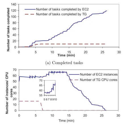
FIGURE 1.6

Usage mode III, Resilience. (a) Allocation of tasks to TeraGrid CPUs and EC2 nodes. As the 16 allocated TeraGrid CPUs become unavailable after only 70 minutes rather than the planned 800 minutes, the bulk of the tasks are completed by EC2 nodes. (b) Number of TeraGrid cores and EC2 nodes as a function of time. Note that the TeraGrid CPU allocation goes to zero after about 70 minutes causing the autonomic scheduler to increase the EC2 nodes by 8.

changed, causing the autonomic scheduler to re-plan and reschedule. Specif-ically, in our experiments, the autonomic scheduler begins by requesting 16 TeraGrid CPUs for 800 minutes. However, after about 50 minutes of execution (i.e., 3 Tasks were completed on the TeraGrid), the scheduler is notified that only 20 CPU-minutes remain, causing it to re-plan and as a result increase the allocation of EC2 nodes to maintain acceptable TTC.

The results of the experiments are plotted in Figure 1.6 and Figure 1.7. Figure 1.6 (a) shows the cumulative number of tasks completed by TeraGrid

(18)

34.69 5.80 35.50 6.60 0 5 10 15 20 25 30 35 40

Runtime in minutes Cost in USD

Normal Model Resilience Mode

FIGURE 1.7

Overheads of resilience on TTC and TCC.

and EC2 over time. As per the original plan, the expected distribution of tasks was 63:65 for TeraGrid:EC2. However, this distribution changes as the TeraGrid resource becomes unavailable, as shown in Figure 1.6 (b), causing EC2 nodes to take up a much large proportion of the tasks. Based on the scheduling policy used, the autonomic scheduler decided that the best TTC will be achieved by increasing the number of EC2 nodes by 8, from 58 originally allocated to 64. The resulting TTC and TCC are plotted in Figure 1.7.

As is probably obvious, the ability to support resilience is a first-step in the direction towards graceful fault-tolerance, but we will discuss fault-tolerance in a separate work.

1.6 Acceleration Usage Mode: Application and

Infras-tructure Adaptivity

1.6.1 Dynamic Execution and Adaptivity of EnKF

We consider two types of adaptivity in this section: infrastructure and ap-plication adaptivity. Infrastructure adaptivity allows the autonomic selection of the appropriate number and type of resources based on requirements and constraints. Application adaptivity adjusts the application behavior based on application/system characteristics (e.g., the size of ensemble members, prob-lem size and application configuration) and runtime state.

(19)

Infrastructure adaptivity is achieved by estimating each ensemble mem-ber’s runtime on available resources and selecting the most appropriate re-sources for them. To estimate runtime on each different resource class, the CometCloud autonomic scheduler asks a worker per resource class to run the runtime estimation module. A worker running on each resource class pulls the task, executes it and returns the estimated runtime back to the scheduler.

If there are no active workers on a resource class, the scheduler launches one. The computational cost of running an estimation task is roughly 5% of that of an actual task. However, if the scheduler needs to start a new worker for estimation, it can incur additional some time delays. A good example would be the overhead of launching a new EC2 instance, or the waiting time in a queue after submitting a pilot job for TeraGrid. This runtime estimation is performed at the beginning of every stage because stages are non-uniform and the runtime of the a stage can not be used as an estimate for the subsequent stage. Once the autonomic scheduler gathers estimated runtimes from all resource classes, it maps the ensemble members (encapsulated as asks) to the most appropriate available resource class based on the defined policy. Policies determine whether runs are made with deadline-based or cost-based (i.e. with budget limits) objectives. The scheduler then decides the number of nodes/workers for each resource class and the appropriate mix of resources. Naturally, workers can consume more than one task and the number of workers is typically smaller than the number of tasks.

Application adaptivity on the other hand relies heavily on the applica-tion infrastructure. Since the reservoir simulator is based on PETSc [4], we have access to a wide variety of direct and iterative solvers and precondition-ers. The selection of optimal solver and preconditioner combination depends on the problem (stiffness, linearity, properties of the system of equations, etc...) as well as the underlying infrastructure. Since the simulator needs to perform several iterations, the first few iterations are performed with sev-eral solver/preconditioner combinations. Thisoptimizationstudy is performed with ensemble member rank 0 only, typically a reference or base–case from which all other ensemble members are generated. The combination with the best performance (shortest wall-clock time) is then selected and passed on to the next stage to reduce simulation runtime.

The overall system architecture used in the experiments is shown in Fig-ure 1.1. Every stage of the application workflow is heterogeneous, and as a result, the selection of infrastructure and application configurations for each stage can be different. At every stage, the autonomic manager collects in-formation about both, the infrastructure and the application, and analyzes this information to decide on appropriate resources and application configu-ration. These decisions affect both current stages (infrastructure adaptivity) as well as subsequent stages (application adaptivity). After reaching a deci-sion on the most efficient infrastructure/application configurations and mix of resources, resources are provisioned andensemble-member-workersare ex-ecuted. On the EC2, this translates to launching appropriate VMs running

(20)

custom images. On the TeraGrid, ensemble-member-workers are essentially

pilot jobs[19] that are inserted into the queue. The workflow manager inserts tasks into CometCloud and ensemble-workers directly access CometCloud and retrieve tasks based on the enforced scheduling policy. TeraGrid workers are allowed to pull the largest tasks first, while EC2 workers pull the smallest tasks. While this policy is not optimal, it was sufficient for our study. During the execution, the workflow manager monitors the executions of the tasks to determine progress and to orchestrate the execution of the overall workflow. The autonomic scheduler also monitors the status of the resources (using the agents), and determines progress to ensure that the scheduling objectives and policies/constraints are being satisfied, and can dynamically change resources allocation if they cannot be satisfied.

It is possible that a defined user objective (e.g. meet a tight deadline) can-not be met. This could be due to insufficient resources for the computational load as a consequence of the deadline imposed; or it could be due to autonomic scheduling efficiency. In addition to the efficiency of the autonomic scheduler (which we do not analyze here), the relative capacity of the TeraGrid & EC2 resources will determine the maximum value of acceleration possible for a given workload. In other words, with the addition of sufficiently large number of cloud resources – possibly of different types of clouds, any imposed deadline will be met for a given workload.

1.6.2 Experiment Background and Set-Up

Our experiments are organized with the aim of understanding how appli-cation and infrastructure adaptivity facilitate desired objectives to be met. Specifically, we investigate how adaptivity – application, infrastructure, or both, enable lowering of the TTC, i.e., acceleration. We explore, (1) how the autonomic scheduler reduces TTC when a deadline is specified, and 2) how adaptation helps achieve the desired objective by facilitating an optimized application and/or infrastructure configuration, or via autonomic scheduling decisions when multiple types of cloud resources are available.

We use a small number of stages of the EnKF workflow with a finite dif-ference reservoir simulation of problem size 20×20×20 grid points and 128 ensemble members with heterogeneous computational requirements. Our ex-periments are performed on the TeraGrid (specifically Ranger) and several instance types of EC2. Table 1.2 shows the EC2 instance types used for ex-periments. We assume that a task assigned to a TeraGrid node runs on all 16 cores for that node (for Ranger).

TeraGrid provides better performance than EC2, but is also the relatively more restricted resource – in that there are often queuing delays. Hence, we use EC2 which is available immediately at a reasonable cost to accelerate the solution of the problem. A task pulled by EC2 node runs sequentially (in case of m1.small which has a single core), or in parallel (other instance types with multiple cores) inside a single VM. To enable MPI runs on multi-core EC2

(21)

TABLE 1.2

EC2 instance types used in experiments

Instance type Cores Memory(GB) Platform(bit) cost($/hour)

m1.small 1 1.7 32 0.1

m1.large 2 7.5 64 0.34

m1.xlarge 4 15 64 0.68

c1.medium 2 1.7 32 0.17

c1.xlarge 8 7 64 0.68

instance, we created a MPI-based image on EC2. This image included the lat-est versions of compilers, MPICH2, PETSc and HDF5 and was configured for performance above all else. Although we experimented with using MPI across multiple VMs as described in Section 1.6.5, we exclude using data from ex-periments involving running MPI across VMs in the analysis of understanding the effect of adaptivity; as is expected, due to communication overheads, it displays poor performance as compared to MPI within a single VM.

1.6.3 Baseline: Autonomic Scheduling in Response to

Dead-lines

At first, the scheduler estimates TTC assuming immediate availability of infi-nite TeraGrid resources. The scheduler then decides how much of the workload should be migrated to EC2 in order to meet the given deadline. If the deadline can be met given the estimated TTC (assuming usage of only TeraGrid re-sources), the number of tasks which should be off-loaded onto EC2 is decided and the autonomic scheduler selects the appropriate EC2 instance types to be launched.

The autonomic scheduler has no knowledge of runtime characteristics of tasks on different resources. The scheduler makes decisions based on estimated runtimes obtained from the runtime estimator module. The runtime estimator is a simple utility that launches a full-size ensemble member simulation with a reduced number of iterations to minimize cost. The results of various ensemble members are tabulated and used to predict the full runtime cost of a complete ensemble member simulation.

In this experiment set, we limit EC2 instance types to m1.small and c1.medium, and run the EnKF with 2 stages, 128 ensemble members each. For baseline experiments/performance numbers, we disabled adaptivity based optimization for both application and infrastructure.

Figure 1.8 depicts the TTC for different values of imposed deadlines and thus gives quantitative information on acceleration provided by the autonomic scheduler to meet deadlines. The imposed deadline takes the values of 120, 108, 96, 72 and 24 minutes respectively; this corresponds to 0%, 10%, 20%, 40% and 80% acceleration, based upon the assumption that a deadline of 120 minutes (0% acceleration) corresponds to a TTC when only TeraGrid nodes

(22)

TTC 0 20 40 60 80 100 120 140 120 108 96 72 24 Deadline (minute) Tim e ( m inut e ) stage1 stage2

(a) Time To Completion

Task consumption 0 50 100 150 200 250 300 350 400 450 120 108 96 72 24 Deadline (minute) N u m b er o f t a sks 0 5 10 15 20 25 num b e r of E C 2 node s stage2-TG tasks stage2-EC2 tasks stage1-TG tasks stage1-EC2 tasks stage1-allocated EC2 nodes stage2-allocated EC2 nodes

EC2 Cost 0.0 0.5 1.0 1.5 2.0 2.5 3.0 3.5 4.0 120 108 96 72 24 Deadline (minute) C o s t ($ ) stage1-estimated cost stage2-estimated cost stage1-experimental cost stage2-experimental cost

(b) Task consumption (c) EC2 cost

FIGURE 1.8

Results from baseline experiments (without adaptivity) but with a specified deadline. We run the EnKF with 2 stages, 128 ensemble members and limit EC2 instance types to m1.small and c1.medium. Tasks are completed within a given deadline. The shorter the deadline, the more EC2 nodes are allocated.

are used. Figure 1.8 (a) shows TTC for stage 1 and stage 2 where each stage is heterogeneous and all tasks are completed by the deadline (for all cases).

Figure 1.8 (b) shows the number of tasks completed by the TeraGrid and number off-loaded onto EC2, as well as the number of allocated EC2 nodes for each stage. As the deadline becomes shorter, more EC2 nodes are allo-cated, hence, the number of tasks consumed by EC2 increases. Since m1.small instances have relatively poorer performance compared to c1.medium, the autonomic scheduler only allocates c1.medium instances for both stages. Fig-ure 1.8 (c) shows costs incurred on EC2. As more EC2 nodes are used for shorter deadlines, the EC2 cost incurred increases. The results also show that most tasks are off-loaded onto EC2 in order to meet the “tight” deadline of finishing within 24 minutes.

(23)

1.6.4 Track 1: Infrastructure Adaptations

The goal of this experiment, involving infrastructure-level adaptivity is to investigate advantages – performance or otherwise, that may arise from the ability to dynamically select appropriate infrastructure, and possibly vary them between the heterogeneous stages (of the application workflow). Specif-ically, we want to see if any additional acceleration (compared to the baseline experiments) can be obtained. In order to provide greater variety in resource selection, we include all EC2 instance types from Table 1.2; these can be selected in stage 2 of the EnKF workflow.

Figure 1.9 shows TTC and EC2 cost, with and without infrastructure adaptivity. Overall, TTC decreases when more resource types are available and infrastructure adaptivity is applied; this can be understood by the fact that the autonomic scheduler can now select more appropriate resource types to utilize. There is no decrease in the TTC when using infrastructure adaptivity for a deadline of 120 because all tasks are still completed by TeraGrid node (since it represent 0% acceleration).

The difference between the TTC with and without infrastructure-level adaptivity, decrease as the deadline becomes tighter; results show almost no savings with the 24 minutes deadline. This is mostly due to the fact that with a 24 minute deadline, a large number of nodes are allocated thus no further gain can be obtained through infrastructure adaptivity.

Figure 1.9 (b) shows the number of nodes allocated for each run and the cost of their usage. The autonomic scheduler selects only c1.xlarge to use for infrastructure-adaptive runs because the runtime estimator predicts that all tasks will run fastest on c1.xlarge. On the other hand, the scheduler selects only c1.medium for non-adaptive runs. Infrastructure-adaptive runs cost more than non-adaptive runs, roughly 2.5 times more at the 24 minute deadline even though the number of nodes for non-adaptive runs is larger than the number of nodes for infrastructure-adaptive runs. This is because the hourly cost of c1.xlarge is much higher than c1.medium (see Table 1.2) and both TTCs are rather short (less than half hour). Since we used deadline-based policy, the autonomic scheduler selects the best performing resource regardless of cost; however, when we switch policies to include economic factors in the autonomic scheduler decision making (i.e., considering TTC as well as cost for 24 minutes deadline), the scheduler selects c1.medium instead of c1.xlarge.

1.6.5 Track 2: Adaptations in Application Execution

In this experiment we run ensemble member rank 0 with variations in solvers/preconditioners and infrastructure. In each case, ensemble rank 0 was run with a solver (generalized minimal residual method GMRES, conjugate gradient CG or biconjugate gradient BiCG), a preconditioner (block Jacobi or no preconditioner) for a given problem size with a varying number of cores

(24)

Infrastructure Adaptivity (stage2) 0 20 40 60 80 100 120 140 120 108 96 72 24 Deadline (minute) Tim e ( m inut e ) non-adaptive runtime infrastructure-adaptive runtime

EC2 Cost (stage2)

0.0 2.0 4.0 6.0 8.0 10.0 12.0 14.0 120 108 96 72 24 Deadline (minute) C o s t ($ ) 0 5 10 15 20 25 30 35 num b e r of node s non-adaptive cost infrastructure-adaptive cost infra-adaptive number of c1.xlarge non-adaptive number of c1.medium

(a) Time To Completion (b) EC2 cost

FIGURE 1.9

Experiments with infrastructure adaptivity. We limit EC2 instance types to m1.small and c1.medium for non-adaptive run and use all types described in Table 1.2 for infrastructure-adaptive run. The TTC is reduced with infras-tructure adaptivity at additional cost.

(1 through 8). Two infrastructure solutions were available: a single c1.xlarge or 4 c1.medium instances.

Figure 1.10 shows the time to completion of an individual ensemble mem-ber, in this case the ensemble rank 0 with various solver/preconditioner com-binations. We varied over two different types of infrastructure, each with 4 different core counts (1,2,4 and 8) and three problem sizes. We investigated six combinations of solvers and preconditioners over the range of infrastruc-ture. Naturally, there is no one, single, solver/preconditioner combination that works for all problem sizes, infrastructures and core counts. Note the experi-ments were carried out on different infrastructure, but the infrastructure was notadaptively varied. For example, Figure 1.10 (c) shows that a problem of size 40x20x20 is best solved on 4 cores in a c1.xlarge instance with a BiCG solver and a block Jacobi preconditioner. This is different from the 2 core, BiCG solver and no preconditioner combination for a 20×10×10 problem on a c1.medium VM as seen in Figure 1.10 (a).

Basic profiling of the application suggests that most of the time is spent in the solver routines, which are communication intensive. As there is no dedicated, high bandwidth, low latency interconnect across instances, MPI performance will suffer, and subsequently MPI intensive solvers. The collective operations in MPI are hit hardest, affecting Gram-Schmidt orthogonalization routines adversely. Conjugate gradient solvers on the other hand are optimal for banded diagonally dominant systems (as is the case in this particular problem) and require less internal iterations to reach convergence tolerance.

From Figure 1.10 we see that as the problem size increases (moving from left to right), the performance profile changes. Comparison of the profiling

(25)

Scaling for 20x10x10 0 100 200 300 400 500 600 700 1 2 4 8

Number of cores (c1.medium, 2 cores per VM)

Ti m e (s ec on ds ) .. 20x10x10_gmres_none 20x10x10_cg_none 20x10x10_bicg_none 20x10x10_gmres_bjacobi 20x10x10_cg_bjacobi 20x10x10_bicg_bjacobi Scaling for 20x10x10 0 10 20 30 40 50 60 70 1 2 4 8

Number of cores (c1.xlarge, 8 cores per VM)

Ti m e (s ec on ds ) .. 20x10x10_gmres_none 20x10x10_cg_none 20x10x10_bicg_none 20x10x10_gmres_bjacobi 20x10x10_cg_bjacobi 20x10x10_bicg_bjacobi

(a) Problem size 20×10×10

Scaling for 20x20x20 0 100 200 300 400 500 600 700 800 900 1000 1 2 4 8

Ti m e (s ec on ds ) .. 20x20x20_gmres_none_{20x20x20_cg_none} 20x20x20_bicg_none 20x20x20_gmres_bjacobi 20x20x20_cg_bjacobi 20x20x20_bicg_bjacobi Scaling for 20x20x20 0 50 100 150 200 250 300 1 2 4 8

Ti m e (s ec on ds ) .. 20x20x20_gmres_none 20x20x20_cg_none 20x20x20_bicg_none 20x20x20_gmres_bjacobi 20x20x20_cg_bjacobi 20x20x20_bicg_bjacobi (b) Problem size 20×20×20 Scaling for 40x20x20 0 200 400 600 800 1000 1200 1 2 4 8

Ti m e (s ec on ds ) .. 40x20x20_gmres_none 40x20x20_cg_none 40x20x20_bicg_none 40x20x20_gmres_bjacobi 40x20x20_cg_bjacobi 40x20x20_bicg_bjacobi Scaling for 40x20x20 0 50 100 150 200 250 300 350 400 450 500 1 2 4 8

Ti m e (s ec on ds ) .. 40x20x20_gmres_none 40x20x20_cg_none 40x20x20_bicg_none 40x20x20_gmres_bjacobi 40x20x20_cg_bjacobi 40x20x20_bicg_bjacobi (c) Problem size 40×20×20 FIGURE 1.10

Time to completion for simulations of various sizes with different solvers (GM-RES, CG, BiCG) and block-Jacobi preconditioner. Benchmarks ran on EC2 nodes with MPI. Problem size increases going from left to right. The top row is for a 2 core VM and the bottom row is for an 8 core VM.

(26)

Application Adaptivity (stage2) 0 20 40 60 80 100 120 140 120 108 96 72 24 Deadline (minute) Tim e ( m inut e ) non-adaptive runtime application-adaptive runtime

0.0 0.5 1.0 1.5 2.0 2.5 3.0 3.5 4.0 120 108 96 72 24 Deadline (minute) C o s t ($ ) 0 5 10 15 20 25 num b e r of node s non-adaptive cost application-adaptive cost number of c1.medium

FIGURE 1.11

Experiments with application adaptivity. The optimized application option is used for application-adaptive run. The TTC is reduced with application adaptivity for equivalent or slightly less cost.

data suggests that a smaller percentage of simulation time is spent in commu-nication as the problem size increases. This is obviously due to the fact that there are larger domain partitions for each instance to work on. Detailed pro-filing of inter–instance MPI bandwidth and latency is still underway, however, early results suggest that this trend continues.

Figure 1.11 shows (a) TTC and (b) EC2 cost using application adaptivity. Applying an optimized application configuration reduces TTC considerably. Application configuration does not affect the selection of infrastructure and the number of nodes, hence, the cost depends on TTC. However, since EC2 costs are billed on an hourly basis (with a minimum of one hour), the decrease in cost does not match the decrease in TTC. For example, with a 108 minute deadline, the time difference between non-adaptive mode and application-adaptive mode is more than one hour. Hence, the cost of application-application-adaptive mode is almost halved. However, because TTCs are all within one hour for other deadlines, EC2 costs remain constant.

1.6.6 Track 3: Adaptations at the Application and

Infras-tructure Levels

In this experiment set, we explore both infrastructure as well as application-level adaptivity. We try infrastructure-application-level adaptivity in the first stage, fol-lowed by application-level adaptivity in the second stage and hybrid adaptivity in the third stage. In principle the final performance should not be sensitive to the ordering. We will compare hybrid-adaptivity to application-adaptivity, as well as infrastructure-adaptivity.

(27)

Hybrid Adaptivity (stage3) 0 20 40 60 80 100 120 140 120 108 96 72 24 Deadline (minute) Tim e ( m inut e ) infrastructure-adaptive runtime application-adaptive runtime hybrid-adaptive runtime

0.0 1.0 2.0 3.0 4.0 5.0 6.0 7.0 8.0 9.0 10.0 120 108 96 72 24 Deadline (minute) C o s t ($ ) 0 5 10 15 20 25 num b e r of node s application-adaptive cost infrastructure-adaptive cost hybrid-adaptive cost number of c1.medium number of m1.xlarge number of c1.xlarge

FIGURE 1.12

Experiment with adaptivity applied for both infrastructure and application. The TTC is reduced further than with application or infrastructure adaptivity on its own. The cost is similar to that in infrastructure adaptivity for durations less than one hour since EC2 usage is billed hourly with a one hour minimum.

Figure 1.12 shows TTCs and EC2 costs; the white columns correspond to infrastructure adaptivity TTC (stage 1), the light blue columns correspond to application adaptivity TTC (stage 2) and the dark blue columns correspond to hybrid adaptivity TTC. As mentioned earlier, the application spends most of its time in the iterative solver routine. The application also runs twenty time-steps for each of the 128 simulations. Therefore, the potential for improvement in TTC from solver/preconditioner selection is substantial. As we expect, the TTC of infrastructure-adaptive runs are larger than those of application-adaptive runs, especially since infrastructure adaptivity occurs once per every stage and application adaptivity influences every solver iteration. As is evident from Figure 1.12 (a), both infrastructure and application adaptivity result in TTC reduction, and even more so when used simultaneously.

The cost for using infrastructure adaptivity is higher than that of using application adaptivity as seen in Figure 1.12 (b). This is due to the simple fact that application adaptivity improves the efficiency of the application without the need for an increase in resources. It is worth mentioning that ours is a special case as the application depends heavily on a sparse matrix solve with an iterative solver. Other applications that use explicit methods cannot make use of application adaptivity (no solvers).

(28)

1.7 Conclusion

Given that production computational infrastructures will soon provide a hy-brid computing environment that integrates traditional HPC Grid services with on-demand Cloud services, understanding the potential usage modes of such hybrid infrastructures is important. In this chapter, we experimentally investigated, from an application’s perspective, possible usage modes for in-tegrating HPC Grids and Clouds as well as how autonomic computing can support these modes. Specifically, we used an EnKF workflow with the Comet-Cloud autonomic Comet-Cloud engine on a hybrid platform, to investigate three usage modes (i.e., autonomic objectives) – acceleration, conservation and resilience. Note that our objective in the experiments presented was to understand each of the usage scenarios and their feasibility, behaviors and benefits, and not to optimize the performance of any one scenario (or experiment). We then focus on acceleration usage modes and explore application or/and infrastruc-ture adaptivity. We show that application and infrastrucinfrastruc-ture adaptivity affect performance and cost.

The results of experiments demonstrate that a policy driven autonomic substrate, such as the autonomic application workflow management frame-work and pull-based scheduling supported by CometCloud, can effectively support the usage modes (objectives) investigated here. The approach and infrastructure used can manage the heterogeneity and dynamics in the behav-iors and performance of the platforms (i.e., EC2 and TeraGrid). Our results also demonstrate that defining appropriate policies that govern the specifics of the integration is critical to realizing the benefits of the integration. The ex-perimental results for investigating adaptivity show that time-to-completion decreases with both system or application-level adaptivity. We also observe that the time-to-completion decreases further when applying both the system and application-level adaptivity. Furthermore, while EC2 cost decreases when application adaptively is applied, it increases when infrastructure adaptivity is applied. This is despite a reduced time-to-completion, and is attributed to the use of more expensive instance types.

While our work so far has been focused on the EnKF inverse problem workflow which is a fairly straightforward, linear workflow complex workflows such as parameter or model space survey workflows can be similarly scheduled. It will be interesting to extend the concepts and insight gained from this work to high-throughput Grids where the individual resources involved will have similar performance to EC2. Additionally the objectives for high-throughput Grids would also be different and so would be the policies required to support the objective.

(29)

Acknowledgment

The research presented in this paper is supported in part by National Science Foundation via grants numbers IIP 0758566, CCF-0833039, DMS-0835436, CNS 0426354, IIS 0430826, and CNS 0723594, by Department of Energy via grant numbers DE-FG02-06ER54857 DE-FG02- 04ER46136 (UCoMS), by a grant from UT Battelle, and by an IBM Faculty Award, and was conducted as part of the NSF Center for Autonomic Computing at Rutgers University. Experiments on the Amazon Elastic Compute Cloud (EC2) were supported by a grant from Amazon Web Services and CCT CyberInfrastructure Group grants.

(30)

(31)

[1] http://www.teragrid.org/.

[2] Amazon elastic compute cloud. http://aws.amazon.com/ec2/.

[3] SPRUCE: Special PRiority and Urgent Computing Environment. http://spruce.teragrid.org/.

[4] Satish Balay, Kris Buschelman, William D. Gropp, Dinesh Kaushik, Matthew G. Knepley, Lois Curfman McInnes, Barry F. Smith, and Hong Zhang. PETSc Web page, 2001. http://www.mcs.anl.gov/petsc. [5] John Brevik, Daniel Nurmi, and Rich Wolski. Predicting bounds on

queuing delay for batch-scheduled parallel machines. InPPoPP ’06: Pro-ceedings of the eleventh ACM SIGPLAN symposium on Principles and practice of parallel programming, pages 110–118, New York, NY, USA, 2006. ACM.

[6] Cactus Framework. http://www.cactuscode.org.

[7] Nicholas Carriero and David Gelernter. Linda in context. Commun. ACM, 32(4):444–458, 1989.

[8] Yaqing Gu and Dean S. Oliver. The ensemble kalman filter for contin-uous updating of reservoir simulation models. Journal of Engineering Resources Technology, 128(1):79–87, 2006.

[9] Yaqing Gu and Dean S. Oliver. An iterative ensemble kalman filter for multiphase fluid flow data assimilation. SPE Journal, 12(4):438–446, 2007.

[10] R. E. Kalman. A new approach to linear filtering and prediction problems.

Transactions of the ASME Journal of Basic Engineering, (82 (Series D)):35–45, 1960.

[11] Hyunjoo Kim, Shivangi Chaudhari, Manish Parashar, and Christopher Marty. Online risk analytics on the cloud. InCluster Computing and the Grid, 2009. CCGRID ’09. 9th IEEE/ACM International Symposium on, pages 484–489, May 2009.

(32)

[12] Hyunjoo Kim, M. Parashar, D.J. Foran, and Lin Yang. Investigating the use of autonomic cloudbursts for high-throughput medical image regis-tration. InGrid Computing, 2009 10th IEEE/ACM International Con-ference on, pages 34 –41, 2009.

[13] Xin Li, Christopher White, Zhou Lei, and Gabrielle Allen. Reser-voir model updating by ensemble kalman filter-practical approaches us-ing grid computus-ing technology. In Petroleum Geostatistics 2007, Cas-cais,Portugal, August 2007.

[14] Zhen Li and Manish Parashar. A computational infrastructure for grid-based asynchronous parallel applications. InHPDC ’07: Proceedings of the 16th international symposium on High performance distributed com-puting, pages 229–230, New York, NY, USA, 2007. ACM.

[15] Paul Marshall, Kate Keahey, and Tim Freeman. Elastic site: Using clouds to elastically extend site resources. Cluster Computing and the Grid, IEEE International Symposium on, 0:43–52, 2010.

[16] S. Ostermann, R. Prodan, and T. Fahringer. Extending grids with cloud resource management for scientific computing. InGrid Computing, 2009 10th IEEE/ACM International Conference on, pages 42 –49, oct. 2009. [17] Cristina Schmidt and Manish Parashar. Squid: Enabling search in

dht-based systems. J. Parallel Distrib. Comput., 68(7):962–975, 2008. [18] Ion Stoica, Robert Morris, David Liben-Nowell, David R. Karger,

M. Frans Kaashoek, Frank Dabek, and Hari Balakrishnan. Chord: A scalable peer-to-peer lookup protocol for internet applications. InACM SIGCOMM, pages 149–160, 2001.

[19] Douglas Thain, Todd Tannenbaum, and Miron Livny. Distributed com-puting in practice: The condor experience. Concurrency and Computa-tion: Practice and Experience, 17:2–4, 2005.

[20] C. Vazquez, E. Huedo, R.S. Montero, and I.M. Llorente. Dynamic provi-sion of computing resources from grid infrastructures and cloud providers. In Grid and Pervasive Computing Conference, 2009. GPC ’09. Work-shops at the, pages 113 –120, may 2009.

Exploring the Use of Hybrid HPC-Grids/Clouds Infrastructure for Science and Engineering

1