Does Partisan Alignment Affect the Electoral Reward of Intergovernmental Transfers?

Does Partisan Alignment Affect the Electoral

Reward of Intergovernmental Transfers?

A

LBERT

S

OLÉ

-O

LLÉ

P

ILAR

S

ORRIBAS

-N

AVARRO

CES

IFO

W

ORKING

P

APER

N

O

.

2335

C

ATEGORY

2:

P

UBLIC

C

HOICE

J

UNE

2008

An electronic version of the paper may be downloaded • from the SSRN website: www.SSRN.com • from the RePEc website: www.RePEc.org • from the CESifo website: Twww.CESifo-group.org/wpT

CESifo

Working Paper No. 2335

Does Partisan Alignment Affect the Electoral

Reward of Intergovernmental Transfers?

Abstract

In this paper we test the hypothesis that intergovernmental grants allocated to co-partisans

buy more political support than grants allocated to local governments controlled by opposition

parties. We use a rich Spanish database containing information about the grants received by

617 municipalities during the period 1993-2003 from two different upper-tier governments

(

Regional

and

Upper-local

), as well as data of municipal voting behaviour at three electoral

contests held at the different layers of government during this period. Therefore, we are able

to estimate two different vote equations, analysing the effects of grants given to aligned and

unaligned municipalities on the vote share of the incumbent party/parties at the regional and

local elections. We account for the endogeneity of grants by instrumenting them with the

average amount of grants distributed by upper-layer governments. The results suggest that

grants given to co-partisans buy some political support, but that grants given to opposition

parties do not bring any votes, suggesting that the grantee reaps as much political credit from

intergovernmental grants as the grantor.

JEL Code: D72, H73.

Keywords: voting, parties, grants.

Albert Solé-Ollé

University of Barcelona

Department of Economics

Avda. Diagonal 690, torre 4, planta 2

08034 Barcelona

Spain

[email protected]

Pilar Sorribas-Navarro

University of Barcelona

Department of Economics

Avda. Diagonal 690, torre 4, planta 2

08034 Barcelona

Spain

[email protected]

We acknowledge the comments made by Benny Geys, Arye Hillman, Barry Weingast, and

other participants at the WZB Conference ‘New Perspectives on Fiscal Federalism:

Intergovernmental Relations, Competition and Accountability’, Berlin, October 18-20 2007.

This paper has benefited from the financial support of SEJ2006-15212 (Spanish Ministry of

Education and Science) and the project 2005 SGR 000285 (Generalitat de Catalunya).

1. Introduction

In recent years, there has been a surge in the empirical literature that seeks to explain the political motives determining the allocation of intergovernmental grants and other public spending programs. For example, adopting the line taken by the theoretical studies of Lindbeck & Weibull (1987) and Dixit & Londregan (1998), the research undertaken by Case (2001), Strömberg (2007), Johansson (2003) and Dahlberg & Johansson (2004) provides some empirical evidence to suggest that more grants are allocated to jurisdictions in which the electors have been shown to be relatively indifferent to the incumbent and the challenger (i.e., there is a high proportion of ‘swing voters’). Some of these papers have sought to contrast this hypothesis with an alternative theory (derived from Cox & McCubbins, 1986) that claims that – if politicians are risk averse – funds will be allocated to those jurisdictions in which voters are clearly attached to the incumbent party (the ‘core supporters’). The results in Dahlberg & Johansson (2004) and Castells & Solé-Ollé (2005) suggest that the evidence in favour of this hypothesis is rather weak, although, as Rodden & Wilkinson (2004) point out, the task of separating the ‘swing voter’ and ‘core supporter’ hypotheses is not easy.

However, this literature misses a fundamental point, which is especially important when dealing with intergovernmental transfers. The models used to date assume that the grantor government is able to get all the political credit arising from the allocation of a grant to a given jurisdiction. However, it often happens that the grant is allocated by the upper layer of government, but the project funded is implemented by the local government, who in this way can stand before the citizens as the main responsible for the expenditure. This is clearly not a problem for the grantor if the local government belongs to the same party, but it can have adverse consequences when there is no partisan alignment, since the grants sent to a jurisdiction to improve electoral chances can actually improve those of the opposition. This argument has recently been proposed by Arulampalam et al. (2008) and Solé-Ollé & Sorribas-Navarro (2007), who use it to obtain the theoretical prediction that grantors will allocate more grants to aligned local governments than they will to unaligned ones. The two papers present empirical evidence to support this hypothesis for India and Spain, respectively. In the Spanish case, Solé-Ollé & Sorribas-Navarro (2007) show that municipalities aligned with an upper layer of government receive up to 40% more grants than those that are unaligned, a figure similar to that reported by Weingast et al.

(2006) for Mexico. The Spanish results are robust across several specifications and, therefore, both the reliability and the size of the effect suggest that something important is going on. It is also worth mentioning that other papers –not making any specific statement about the behavioural reason of the finding– did previously find, for other countries, that ideology matters

in the allocation of grants and other public programs (see, e.g., Grossman, 1994; and Levitt & Snyder, 1995).

But while the evidence is compelling, nothing is known about the underlying motives that make grantors behave the way they do. As discussed above, papers by Arulampalam et al. (2008) and Solé-Ollé & Sorribas-Navarro (2007) suggest that the answer lies in the ‘differential productivity’ of grants allocated to aligned vs. unaligned governments. Others, however, suggest that ‘clientelism’ is the reason of the biased allocation of transfers, non-aligned governments being punished by withdrawing transfers in order to force the population to dismiss the incumbent in the following election (see, e.g., Weingast et al., 2006). Note that this second hypothesis requires much more rationality on the part of the voters, whose voting decision is based not on the retrospective evaluation of monies received but on the expected future value of grants (which will be higher if there is alignment). Moreover, although the ‘clientelist’ channel cannot be totally discarded in Spain (see e.g., Cazorla, 1995), the low share of revenues funded by discretionary grants, and the fact that there are several grantors controlled usually by different parties (see section 3.1), suggest that the threat of punishment is not particularly great in Spain and that the first explanation (‘differential productivity’) is more plausible. Therefore, in this paper we will concentrate in finding direct evidence that grants allocated to aligned governments result in more votes than grants allocated to the unaligned ones. We believe there is real value added on this exercise, since we don’t know of any previous attempt to find evidence regarding this issue.

Moreover, the data we use to test this hypothesis is particularly well suited to this purpose. We use a rich Spanish database, which provides information on capital grants received by 617 municipalities during the period 1993-2003 from two different upper-tier governments (i.e.,

Regional and Upper-local) and municipal vote data on three electoral contests held during this period at the municipal an regional layers. Therefore, we are able to estimate two different vote equations that analyse the effects of grants given to aligned and unaligned municipalities by different upper layers of government on the vote share of the incumbent party/parties at the local and regional elections. We account for the endogeneity of grants by instrumenting them with the average amount of grants distributed by upper layer governments. We focus our analysis on capital grants because these are grants that are earmarked for very specific purposes and that should be solicited to the upper layer, which has some discretion in the selection of projects, meaning that political factors could play a role in its allocation. Note also that in the case of these capital grants both layers of government share the responsibilities for the service (e.g., the upper layer sets the eligibility criteria and provides the funds, and the lower layer implements the project and co-funds). This means that both layers are seen by the voters as

party responsible for the service, and suggests that the allocation of these grants is likely to respond to differential electoral productivity3_{. The results of the empirical analysis suggest that}

grants given to co-partisans buy some political support, but that grants given to opposition parties do not bring any votes, suggesting that the grantee reaps as much political credit from intergovernmental grants as the grantor.

The paper is organized as follows. In the second section we present a theoretical framework that will allow us to motivate the vote share equation to be estimated, and to interpret the coefficients obtained for the grants given to aligned and unaligned governments in terms of the ‘differential productivity’ hypothesis introduced above. The third section discusses carefully the econometrics of the exercise, focusing on the potential endogeneity of grants; to this end we use the theoretical framework developed in the previous section to guess the possible direction and magnitude of the bias and to propose a method to solve the problem. In the fourth section we briefly describe the institutional details of the Spanish case that will help to understand why we have adopted this particular empirical strategy. The concrete operationalization of the vote equation and the data used to compute the different variables are presented in the fifth section. The sixth section presents the results obtained. Finally, the paper ends with some conclusions and suggestions for further research on this issue.

2. Theoretical framework

In this section we posit a very simple framework in order to describe how a voter decides his vote, depending on the alignment between the governments at different tiers. The approach used here is the same as that adopted in Solé-Ollé & Sorribas-Navarro (2007), who embed this behaviour in a model of electoral competition in order to derive implications regarding the effect of alignment on the amount of grants allocated. We first describe the basic set-up of the model: layers of government and parties. Then we describe how a voter determines his vote, depending on the alignment between governments at different tiers, and suggest how the vote equation could be specified in the empirical analysis.

Basic set-up. In the model there are two upper-tier governments, each one with a jurisdiction covering the entire country, and a number of local governments. We will call the first tier R

3 _{Nonetheless, it should be noticed that other studies (e.g. Arulampalam et al. 2008) find evidence that}

alignment do have an effect also on the allocation of unconditional grants. This could be due, for example, to widespread central regulations and/or to soft-budget constraint, which make voters think that the ultimate financial backer of the services is the central government. As we will argue at the end of the paper, whether co-partisanship has or not an effect on the allocation of different types of grants might be highly dependent on the details of each country’s federalist institutions.

(Regional) and the second one U (Upper-local). For illustrative purposes, we assume that a different party controls each upper tier government: the R government by the right-wing party (r) and the U government by the left-wing one (l). Some local governmentsare controlled by the

r party and some by the l party. The two parties, r and l, use the financial resources available at the tier of government they control to distribute grants to the local governments and advance their electoral prospects. Although each party controls a different government tier, and different elections are held at each tier, the model assumes that they are competing in the same electoral race, without specifying which specific election we are talking about4_.

Voters’ behaviour. Voters vote on the basis of two criteria: (i) the welfare generated by grants, , with >0 and ≤0, and where are per capita grants in municipality J, coming from R and U, respectively; and (ii) ideology. We define as the ideological bias of voter i in favour of party l, which is unknown to the researcher; is a distribution of , with ) (g_J u '( ) J g u i X ) ( '' J g u = ) i X U J R J J g g g = + i

X

( J X F _i) ( J

f ∂F_J(X_i)/∂X_i, which is common knowledge. There is an additional component in the voting behaviour which is a general popularity shock,

δ

_J, in favour or against the party in the R and U governments, which is municipality-specific (but common to all voters) and known before grants are determined. We assume that voter i votes for party r if 5 J δ + i X ≥ U J R_)−u(g J g u( ) .

Now we assume that the voting decision of voter i depends on the alignment status of her local government. Following Arulampalam et al. (2008), we define θ as the proportion of utility from grants that the voter attributes to the local government and (1–θ) as the proportion of utility from grants attributed to the grantor upper layer of government. If both layers are controlled by the same party, then all the utility from grants is captured by this party. If control is split between the two parties, then utility from grants must be shared. Nothing can be a priori said about the value of θ, which will be derived from the estimated vote equation (see below).

4 _{This amounts to assume that politicians at all levels are interested in advancing the prospects of the}

party in general, and not only in winning the elections held at their particular layer of government. This may happen, if campaigns are highly centralized, if the electoral results of a party in a given election and jurisdiction are influenced by the results obtained in other contests, or if winning elections helps the party in rewarding its supporters through the allocation of posts.

5 _{The voter will vote for r if the welfare gain obtained from r during the last term-of-office relative to the}

one obtained from l is higher than the ideological bias in favor of l: ΔuJr-ΔuJl≥Xi+ δJ. This welfare gain is

hypothetical and should be interpreted as the welfare increase derived from grants coming from the government controlled by that party compared to a situation in which all the grants came from the government controlled by the other party. It is only in this case that ΔuJr-ΔuJl reduces to u(gJR)- u(gJU).

Thus, if the incumbent party at municipality J is r, i.e. J is alignedwith R, voter i votes for party r if: 4 43 4 42 1 4 4 3 4 4 2 1 l U J iJ J r U J R J u g X u g g u by captured utility by captured utility ) ( ) 1 ( ) ( ) ( +θ −δ > + −θ or, U _{J i} (1a) J R J u g X g u( )−(1−2θ) ( )−δ >

That is, expression (1) says that if the municipality is aligned with R, all the utility coming from grants allocated by R is captured by the party r but, since the municipality is not aligned with U, also a proportion θ of the grants allocated by U is captured by party r. Similarly, if the incumbent party at municipality J is l, i.e. municipality J is unaligned with R, voter i votes for party r if: 4 4 3 4 4 2 1 4 4 3 4 4 2 1 l R J U J iJ r J R J X u g u g g u by captured utility by captured utility ) ( ) ( ) ( ) 1 ( −θ −δ > + +θ or, U _i (1b) J R J u g X g u − − > −2θ) ( ) ( ) δ 1 (

Expressions (1a) and (1b) suggest that grants from aligned upper layers of government have a much greater impact on the incumbent’s vote (in absolute terms) than grants coming from unaligned governments. In both expressions, grants coming from unaligned governments ( in expression (1a) and in (1b)) are interacted by the term (1-2

U J g R J g θ), which value is

conditioned on the voter’s distribution between the grantor and the grantee of the utility derived from grants. The higher the proportion

θ

of utility attributed to the local government is, the lower the impact of grants coming from unaligned government on the incumbent’s vote share is.

Vote share equation. Now we can combine these two expressions to write the vote-share for the incumbent party at, for instance, the regional government in a municipality, as:

(2) ) ) ( ) 2 1 ( ) ( ( uR _J J aR J J J R J F u g u g v = − − θ −δ

where and are the grants that a local government receives from aligned and unaligned upper layers of government, respectively. Let’s assume that utility is linear in grants (i.e.,

) and define the dummy variables and , which are equal to 1 if the

aR J g g β = uR J g J J g u( ) R J a U J a

regional and upper-local governments are politically aligned with municipality J. Now, from expressions (1a) and (1b) we can write the utility derived from grants in a municipality aligned and unaligned with the regional government as:

) and (3) ) 1 )( 2 1 ( ( U J U J R J R J g a g a − − θ − (1 )((1 2 ) U) J U R J R J g a g a − − − θ

Adding these two expressions and grouping the variables according to the alignment status, the grants received from upper layers of aligned and unaligned government can be expressed as6_:

and (4) U J U J R J R J aR J a g a g g = − U J U J R J R J uR J -a g -a g g =(1 ) −(1 )

Although it is not absolutely necessary to derive our testable hypothesis, the use of a particular vote distribution for will help us to clarify it. For illustrative purposes, if we assume that is normally distributed (i.e., ∼ ), being

) ( _i J X F ) ( _i J X F F_J(X_i) (_μ ,_σ2) J N μ_J a municipal specific mean of the distribution and its variance, which for simplicity we assume constant across municipalities, the vote equation would look like:

2 σ J uR J aR J R J g g v~ =β₁ +β₂ +β₃ρ (5a)

where ρ_J =μ_J+δ_J and v~_J =Φ−1(v_J), standing for the standard normal distribution, and where ) (• Φ

σ

β

β

₁ = / ,

β

₂ =−(

β

/

σ

)(1−2

θ

) and β₃ =−1 /σ . We could use an even simpler approach, assuming F_J(X_i) is uniform with mean μ_J on the support −Ψ+μ_J Ψ+μ_J this case the vote equation is:

, . In (5b) 3 2 1 0 JaR uRJ J R J g g v =β +β +β +β ρ

where 2β₀ =1 / β₁=β /2Ψ, )β₂ =−(β/2Ψ )(1−2θ and β₃ =−1 /2Ψ. Note that the specification obtained is practically the same under both assumptions, with the exception that in the last case it is no longer necessary to apply any transformation to the vote share.

6 _{Note that, since we assume that the regional government is always controlled by the right party and the}

upper-local one by the left party, we have and , meaning that it holds that

and . U J R J a a =1− R J U _a a =1− U R J a a = − ) 1 ( U J R J U J R J a a a a (1− )= =1− (1−a_JR)aU =

It is important to stress that the results of both equations have the same interpretation and allow us to defend the specification of an estimable vote equation to test the hypotheses we made regarding the effect of partisan alignment on voter behaviour. Note that in both expressions (5a and 5b), if β₁>0 and θ <0.5 then we expect β₂ >0 and β₁ > β₂ , if θ =0.5 then β₂ =0 , and if θ >0.5, then β₂ <0 and β₁ > β₂ . That is, if β₁ >0 , grants to aligned municipalities buy votes in all feasible scenarios, but grants to unaligned municipalities might bring or detract votes depending on the distribution of credit between layers of government; if more credit is attributed to the higher layer of government than it is to the lower layer (i.e. θ <0.5), these grants should also bring more votes (although less than grants to co-partisans); if credit is more or less equally split between layers (i.e. θ =0.5), grants to unaligned municipalities will neither bring nor detract votes; and if more credit is attributed to the lower layer (i.e. θ >0.5), these grants will detract votes (although the impact on absolute value will be lower than that of grants to co-partisans). In the extreme case where the grantee does not keep any political credit (i.e.

1

=

θ ) grants will have the same effect on votes independently on whether they come from aligned or unaligned upper layers of government.

Finally, note that a feature of the model is that the results of the elections to the upper tier of government do not only depend on the grants distributed by the level of government analysed, but also on the grants distributed by all levels of government. For instance, the vote-share obtained by the incumbent at the regional government in a municipality depends not only on the grants assigned by the regional government but also on those allocated by the upper local government. This is the result of our assumption that governments are interested in fostering the ‘general interests of the party’ and not only on winning their own election. Although this assumption is, of course, debatable, our results will allow us to test its validity.

3. Econometrics

The main problem in estimating a vote equation based on (5a) or (5b) is the possible endogeneity of grants. The issue can be described in terms of an omitted variable problem, since both the average ideological attachment of the population and the popularity shock of the government will be very difficult to measure. For example, with omitted from (5a) the model estimated will be simply

J ρ

7_:

7 _{For simplicity, in this section in the expressions we omit the subscript that specifies the level of}

J u J a J J g g v~ =γ₀+γ₁ +γ₂ +η with η_J =ρ_J+ε_J (7)

where we add the ε_J i.i.d. term to the equation. Note that, whenever and are correlated with , the coefficients

a J g u J g J

ρ

γ

ˆ₁ and

γ

ˆ₂ will be biased (i.e., will differ from β₁ and

β

₂). In our case this correlation is not just an empirical possibility, but can be a result of the theory. The paper by Solé-Ollé & Sorribas-Navarro (2007), for example, departs from the vote behaviour as described in (2) to derive a prediction regarding the effect of alignment on the amount of grants received. They assume that the objective of each party is to maximize the expected number of votes taking the decision of the other party as fixed (i.e., Nash behaviour) and subject to a fixed budget constraint. The details of the analysis are referred to that paper; here it suffices to note that after analysing the F.O.C. they suggest that a specification such as the following might be appropriate: J a J J a J f g g =λ₁ (ρ )+λ₂ +ξ (8a) J u J J u J f g g =λ₁ (ρ )+λ₂ −Ω+ω (8b)

where is the equilibrium cut-point density (i.e., a measure of the proportion of ‘swing voters’), which depends on the shape of the density function and on the value of the popularity shock, ) ( _J J f ρ a

g and _gu _{are average per capita grants allocated to aligned and unaligned local}

governments, is a constant picking up the effect of alignment (unalignment), Ω λ₁ and λ₂ are positive coefficients, and ξ_J and are i.i.d. error terms. So, theory seems to suggest that popularity shocks (i.e.,

J ω J

ρ ) do have some effects on grants allocated, implying that there could be a possible omitted variable bias problem. The formulas for the bias of the estimated γˆ₁ and

ˆ₂

γ coefficients can be expressed as:

) / ( ). / ( ) ˆ E( _{2 2 2} 2 2 2 2 1 2 1 1 1 ξ ρ ρ σ σ λ σ ρ λ σ ρ λ β γ + + ∂ ∂ ∂ ∂ + = a g J J J J f f (9a) ) / ( ). / ( ) ˆ E( _{2 2 2} 2 2 2 2 1 2 1 2 2 ω ρ ρ σ σ λ σ ρ λ σ ρ λ β γ + + ∂ ∂ ∂ ∂ + = u g J J J J f f (9b)

where 2, ρ σ 2 a g σ , 2 u g

σ , and are the variances of the popularity shock, average grants distributed from aligned and unaligned governments, and error terms of equations (8a) and (8b), respectively. Note that the direction of the bias depends on the sign of

2 ξ σ 2 ω σ J J f ∂ρ ∂ / . Suppose for a moment that this derivative is negative (i.e., the shock decreases the proportion of ‘swing voters’, something that happens on the right-wing side of the density function, once we assume

F is symmetric and single-peaked as in Solé-Ollé & Sorribas-Navarro (2007)); in this case, both coefficients are downward biased, since β₁ is positive and β₂ is expected to be negative or zero. Note also that the bias shall be in both cases of a similar magnitude, whenever 2

a g σ and in (9a) are similar to their counterparts in (9b) (i.e.,

2 ξ

σ 2

u g

σ and 2). This means than if

ω

σ

β

₁ is

higher (in absolute terms) thanβ₂, the OLS estimates of equation (7) should also give γˆ₁>γˆ₂ . Note that if ∂φ_J/∂ρ_J is positive (i.e., the ‘shock’ increases the proportion of ‘swing voters’, something that happens on the left-wing side of the density function) then the coefficients are upward biased; however, it is also plausible that the OLS coefficients say that γˆ₁>γˆ₂ when grants to aligned governments bring more votes than grants to unaligned ones.

But although this is an interesting property, it only allows us to guess if our main hypothesis is valid (i.e., grants to co-partisans buy more support than grants to the opposition), without allowing us to obtain a more precise estimate of the degree to which credit for grants is transferred from the grantor to the grantee; for this we need to gauge the magnitude of the θ parameter, an impossible task given the bias of γˆ₂. It would also be helpful to know something about the direction of the bias, but this depends on the sign of ∂f_J/∂ρ_J. If the density was symmetric and single peaked, and since we know that there is some incumbency advantage (see, e.g., Bosch & Solé-Ollé, 2007b), we can assume that most municipalities are on the right-hand side of f_J, meaning that ∂f_J/∂ρ_J<0. This would mean that there are some arguments to expect that the γˆ coefficients are biased downwards.

However, it would be much better to solve the endogeneity problem. Here we propose the use of an Instrumental Variables procedure. Note that expressions (8a) and (8b) already propose one instrument for each of our endogenous variables; these are simply the average per capita amount of grants distributed by aligned and unaligned higher layers of government (i.e., ga and gu). The intuition here is quite clear: municipalities belonging to regions where Regional and Upper-Local governments distribute huge amounts of grants will, in general, receive more transfers than municipalities belonging to regions where few grants are allocated to local governments. It can be argued convincingly that these two variables do not belong to the vote-share equation.

Note that it is difficult to imagine that the effects of grants could spill over to other municipalities belonging to the same geographical area (i.e., receiving grants from the same upper-layer governments) and controlled by the same party. Therefore, given that it is quite plausible that these instruments are not correlated with the error term

η

_J, their use will allow us to obtain unbiased estimates of the parameters of interest. Moreover, as will be checked in the next section, these instruments have a considerable explanatory capacity in the first-stage regression, allowing us to avoid the problem of weak instruments.

This procedure is similar to that adopted by Levitt and Snyder (1997) for the U.S. case. The only drawback faced by these authors is the impossibility of using over-identification tests to check the validity of the instruments. Although they acknowledge the presence of this problem, they believe that the theoretical justification of the instrument is sufficient to defend its validity. In our case, we will not rely exclusively on intuition to justify the instruments used. Note from (4) that both grants coming from aligned and unaligned grantors could be split in two different components. Similarly, we can divide each of our instruments (_ga _{and g}u_{) in two; for}

example, in the case of _ga _{we now have} R J R J aR _{a g} g = and U J U J aU _{=a g} g

. By having two instruments for each endogenous variable, we are able to compute the Hansen overidentifying restriction test to check the validity of the instruments.

4. Institutional background of Spain

Layers of government and transfers

Spain is a fiscally decentralized country with three layers of government: Central, Regional and

Local. There are seventeen regional governments, the so-called Autonomous Communities (ACs), which have very important spending responsibilities including, for example, the provision of health care, education and welfare. Each AC is composed by one or more provinces. In the ACs composed by more than one province, there exists an upper-tier of local government, called Diputación, referred to here as Upper-Local. Although this upper-tier of local government has fewer spending responsibilities than the municipalities, which are the main players in the local public sector, allocation of grants for capital infrastructure to municipalities is one of their most important tasks8.

8 _{In ACs with only one province (there are six ACs of this kind), there is no Diputación, and its}

Spain has over eight thousand municipalities although most are quite small. Municipalities are multi-purpose governments, with major expenditure categories corresponding to the traditional responsibilities assigned to the local public sector (environmental services, urban planning, public transport, welfare, etc.) with the exception of education, which is a responsibility of the regional government. Current spending is financed out of own revenues (2/3 approx.) and unconditional grants (1/3 approx.) which are allocated by a formula that makes their use difficult for pork-barrel politics. However, the funding of capital spending depends heavily on grants: in 2003, capital grants represented 13% of non-financial revenues and 44% of capital spending. These grants came from the three upper-layers of government: Central (15%),

Regional (45%) and Upper-Local (21%)9_{. Most of the grants take the form of ‘project grants’:}

there is an open call at regular periods (usually yearly) and the municipality must apply by submitting several infrastructure projects. These are evaluated in accordance with pre-established criteria (usually published in the call), but that are, nevertheless, subject to the interpretation of the grantor. Therefore, the degree of political discretion applied to these grants can be qualified as high.

Elections and parties

In Spain, central elections are usually held at regular four-year periods, although they can be called before the end of the term-of-office. Municipal and regional elections are held regularly every four years and on the same day in twelve out of seventeen ACs. In the period analysed, they were called one or two years before the general election. In the other ACs, elections were called before the end of the term and, therefore, were held on a different day.

In the elections to the central and regional legislatures, the electoral districts are the provinces. A different number of representatives is elected in each province depending on its population size; candidates are included in parties’ closed lists; and the d’Hondt formula with a threshold is used to translate the number of votes into the number of representatives (Colomer, 1995). Therefore, the system is not entirely proportional and, in fact, it is much easier to win a seat in some provinces (rural areas) than in others. Due to the closed-list system, parties are highly disciplined, both inside the legislatures and (to a lesser extent) across layers of government. Since the party has a great influence on the future prospects of politicians (through the allocation of posts and places on the lists), they use to be loyal to the constituency but also to the party.

In municipal elections closed lists are also adopted, the number of city councillors depends on population size, and the d’Hondt rule is also used, but in this case there is just a single district. As Colomer (1995) states: “these rules provide incentives for sincere voting and promote a high degree of pluralism in city councils”. As a result, there is a high proportion of coalition governments; for example, in the 1996-99 term 43.3% of the municipalities where governed by coalitions (Solé-Ollé, 2006). Most municipal candidates are aligned along national or regional party lines. The local political system is seen as a first step in the process of recruitment into the regional and national political elite (Magre, 1999). There are no specific elections to the assembly of the upper-tiers of local governments; the representatives of Diputaciones are elected on the basis of the results at the municipal elections. The votes for each party are aggregated across municipalities and the number of representatives is obtained, once again, by using the d’Hondt formula. These upper-tiers of government have been criticised on the grounds of their low level of electoral accountability: with few clear responsibilities and no need to go to the polls, politicians controlling this layer of government can use grants to foster the parties’ prospects at the next municipal election.

The nature of the Spanish electoral and party system described above means that the elections held at each layer of government are not entirely independent of the national or regional political situation. In fact, parties follow the results of regional and municipal elections with great interest. Since these contests are usually held one or two years before the central elections, they provide an excellent occasion to test the real prospects of the party10_{. Therefore, although}

most efforts are focused locally, the parties do design a centralized (national and/or regional) strategy for these contests. This strategy includes statements regarding which regions and/or municipalities deserve greater campaign efforts11_{, either because the perceived electoral margin}

is low or because the region or the city is seen as having special significance in the eyes of voters (e.g., big cities). In the Spanish context, it is therefore natural to believe that just before an election, a party uses the various posts they control at different layers of government to allocate grants to pursue its electoral objectives. The high degree of partisan control exercised both inside and across layers of government facilitates the use of resources coming from different posts for the fulfilment of party interests.

10 _{This is due to the fact that national and/or regional political shocks do affect the results of these lower}

tier elections (see, e.g., Bosch & Solé-Ollé, 2005, and Rodden et al., 2005, for evidence of this effect in Spain and other countries, respectively). In fact, local electoral results are seen as predictors of the parties’ prospects for the next general election.

11 _{One year before the May 2007 municipal elections the newspaper El País published a report on the}

prospects for this contest entitled: “PSOE and PP open the battle town by town” and identified the regions and municipalities where each party would concentrate its efforts (source: El País, 23 April 2006, p. 26: “PSOE y PP abren la batalla pueblo a pueblo”).

5. Empirical analysis

Vote equations

The specification of our vote equation is built upon the results presented above in the theoretical section. Although the Spanish case described above provides us with three upper-tier grantor governments (Central, Regional and Upper-Local), we will only analyse how the election results of the incumbent party/parties at the Regional and Local levels are affected by the grants allocated by the Regional and Upper-Local governments. We decided not to analyse the effects of central grants on the results of these elections and not to analyse the results of the general elections because these grants account for less money than the others and because the improvement of municipal infrastructure plays only a minor role in shaping the electoral agenda of the Spanish general legislative elections. This, however, is not the case of the regional and local elections, since the ACs, the Diputaciones and the municipalities are all responsible for the delivery of these services. Thus, we implicitly assume that the parties use the grants they control at the Upper-Local and Regional layers to influence the results of both the regional and the local elections. We do not analyse the election results of the incumbent at the Upper-Local level, since, as it has been said, there are no direct elections to the Upper-Local governments. Its representatives are elected as a product of the results of the municipal elections.

Thus, as starting point, we will estimate the following two equations:

(10a) R Jt mR Jt R R Jt R R Jt g v =β +α ρ +ε (10b) L Jt mL Jt L L Jt L L Jt g v =β +α ρ +ε

where and are the vote shares of the incumbent party/parties in the Regional (R) and

Local (L) governments in the regional and local elections held at t, respectively; and and are the amounts of total capital grants per capita received by municipality J in the two years prior to election t. That is, = and = . The computation of these variables will be described bellow. This equation allows us to test whether capital grants do have any effect on the vote share. Note that this specification implicitly assumes that the grantee does not keep any political credit and thus, all grants have the same effect (i.e., increase the vote for the municipal incumbent), independently on whether they come from aligned or unaligned governments. R Jt v L Jt v R Jt g L Jt g R Jt g g_JaR+guR_J L Jt g g_JaL+guL_J

Secondly, in order to test our hypothesis that is, that grants allocated to aligned governments result in more votes than grants allocated to the unaligned ones, we will estimate the previous equations, but decomposing the grant variable depending on whether they come from aligned or unaligned governments. This will allow us to infer the value of θ, i.e., the distribution of the political credit of grants among the grantor and the grantee. Thus, we will estimate the following equations: (10c) )

3 2 1R JaR R JtuR JtmR JtR R Jt g g v =β +β +β ρ +ε (10d) 3 2 1L aLJt L uLJt JtmL JtL L Jt g g v =β +β +β ρ +ε

The grant variable labelled with superscript a in expression (10c), , indicates the amount of money per capita received by municipality J in the two years prior to election t from the incumbent at the upper-local and regional governments with whom it is aligned, less –when not aligned with the incumbent at the level of government under analysis– the amount of money per capita received by municipality J from the layers of government with which it is aligned. Thus,

is computed as: aR J g aR Jt g (11) U Jt U Jt R Jt U Jt U Jt R Jt R Jt aR Jt a g a g a a g g = ( + )−(1− )

where and are equal to 1 if the regional and upper-local government are aligned with the municipal government, respectively. The grant variable labelled with superscript u in expression (10c) indicates the amount of grants per capita received by municipality J in the two years prior to election t from the upper level incumbent governments with whom it is unaligned. Thus, is computed as: R Jt a U Jt a uR Jt g (12) ) 1 (( ) ) 1 ( )( 1 ( U Jt U Jt R Jt U Jt U Jt R Jt R Jt uR Jt a g a g a a g g = − + − − −

Note that although these expressions might seem rather complex, these calculations are nothing more than the transposition of expression (4) to a more realistic setting12_{. The intuition behind}

the specification in (11) is that the electoral prospects of the incumbent at some high layer of government increases the more grants it is able to channel to aligned municipalities (coming

12 _{Note that in the real world we should allow for and , since a local}

government can also be aligned or unaligned with both upper layers of governments. U

J R

J a

directly from its budget or from the budgets of other layers of government also controlled by the same party) and the fewer grants other layers of government controlled by the opposition are able to channel to municipalities which are not aligned with it.

It can be argued, of course, that this computation is overly complex, since voters might be able to disentangle the purpose of the different electoral contests and, therefore, only take into account the grants coming from the incumbent at his own election. In other words, and contrary to what expressions (11) and (12) might suggest, only Regional grants have some impact on the vote at regional elections but not Upper-Local grants. This means that politicians would not be able to foster the ‘general interests of the party’ (as we assumed in the theoretical section), using the grants at their disposal to influence elections at any layer of government, but rather they are forced to compete in only one election. To verify this possibility we will decompose expressions (11) and (12) into two different variables. So, we will have grants coming from aligned grantors

computed separately for the Regional and Upper-Local grantor:

(13a) R Jt R Jt aR Jt Regional a g g ( ) = (13b) U Jt U Jt R Jt U Jt R Jt aR Jt Upper Local a a a a g g ( − )=( −(1− ) )

and also grants coming from unaligned grantors computed separately for the Regional and

Upper-Local grantor: (14a) R Jt R Jt uR Jt Regional a g g ( )=(1− ) (14b) U Jt U Jt R Jt U Jt R Jt uR Jt Upper Local a a a a g g ( − )=((1− )(1− )− (1− ))

The four variables will be included in the equation. In the event that only (13a) is statistically significant, we should conclude that grants only have an effect on those elections at which the grantor is the incumbent, and not on elections held at other layers where the incumbent is not the grantor but one of his co-partisans at the other layers.

When analysing the results at the local elections, the expression used to calculate the grants coming from aligned and unaligned governments are the following:

(15) U Jt U Jt R Jt R Jt aL Jt a g a g g = +

(16) U Jt U Jt R Jt R Jt uL Jt a g a g g =(1− ) +(1− )

These expressions are much simpler than the ones defined when analysing the results at the regional election, since the alignment variable is defined in relation to the incumbent at the level of government under analysis. Nonetheless, these expressions capture the same information.

Note, finally, that the vote equations in (10a), (10b), (10c) and (10d) also include a term measuring the ideological attachment of the population and/or the popularity shock experienced by the government, which differs from one equation to the other: and . The m

superscript means that these popularity effects are considered measurable. To account for them we include a set of proxies to be described below. Finally, these equations include an error term composed by an immeasurable shock and an i.i.d disturbance (e.g., ). As this popularity shock can be correlated with the amount of grants received (either from aligned or from unaligned grantors), we face a potential problem of endogeneity for which the use of instrumental variables is recommended, as argued in section 3.1.

mR Jt ρ R Jt ε = mL Jt ρ R Jt η iR Jt ρ + Data description

Selecting the sample. We estimate the effects of grants on the municipal vote share obtained by

the incumbent party/parties at regional and local layer of government. We use a rich database, which provides information about the vote share of parties at different types of elections and about the grants received by 617 municipalities from different grantors during the period 1993-2003. Voting data come from information provided by the Spanish Ministry of the Interior, in the case of the local elections, and directly from each of the Regional governments, in the case of the regional elections. The data on grants come from a survey on budget outlays conducted yearly by the Ministry of Economics and Finance. The initial number of municipalities was much higher (2,799), but we could not use the municipalities with fewer than 1,000 inhabitants due to the lack of socio-economic data, and we also lose some municipalities due to the lack of data on transfers by grantor. Moreover, we only use the municipalities that belong to a region where the Upper-Local government exists. However, we believe that despite this reduction in the number of observations the sample is still representative of Spanish municipalities with more than 1,000 inhabitants, since we checked that the municipalities lost because of the unavailability of the breakdown in transfers are distributed proportionally according to population size and alignment status.

Measuring votes: The vote variables are calculated as the share of votes obtained by the

incumbent party/parties at the Local and Regional government in each municipality at the municipal and regional elections, respectively. To construct these variables we use the electoral results of the municipal and regional elections held in 1991, 1995, 1999 and 2003.

Measuring grants. Our grant variables are capital grants (chapter 7 of the budget) coming from

each upper layer of government (R and U). As we have already said, we only focus our analysis in capital grants, since their distribution is not formula based and, thus, they are more likely to be distributed according to their electoral productivity. Total grants are summed together for the last two years of each term-of-office and then divided by the population of the municipality at the beginning of these two-year periods, using data from the National Institute of Statistics (INE). We have assumed that grants received during the election year benefit the incumbent government and not the incoming one. We believe that this assumption is reasonable, given that municipal elections are generally held in the middle of the year (May or June) and that grantor governments usually exhaust their yearly grants budget early, just before the next election. Thus, we set out to explain the effect of grants on the electoral reward by examining the overall amount of grants received in 1994-95 for the term 1991-95, in 1998-99 for the term 1996-99, and in 2002-03 for the term 2000-03. There are three reasons that justify this decision. The first one is the fact that in some ACs it is not always easy to identify alignment between layers of government given the different timing of regional and local elections. Thus, the alternative procedure of aggregating grants over an entire local term of office would have run into the problem of changing alignment in the middle of a period (since some regional elections are held at a date some time between local elections). The second reason is that by aggregating the grants variable over two years, we reduce the volatility of this variable. The third reason is that, as the political cycle literature has emphasised, the temptation to use public funds to buy votes increases as the next election approaches, suggesting that the electoral reward will be higher in that time period13_.

13 _{See, e.g., Castells & Solé-Ollé (2005) for evidence indicating that pork-barrel politics in Spain}

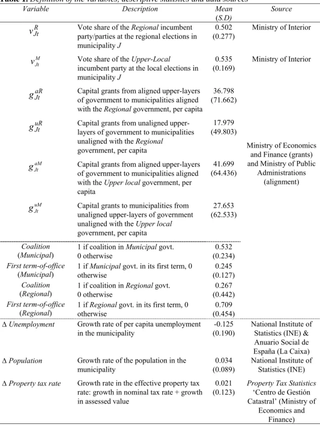
Table 1. Definition of the variables, descriptive statistics and data sources

Variable Description Mean

(S.D)

Source

R Jt

v

Vote share of the Regional incumbent

party/parties at the regional elections in municipality J 0.502 (0.277) Ministry of Interior M Jt

v

Vote share of the Upper-Local

incumbent party at the local elections in municipality J 0.535 (0.169) Ministry of Interior aR Jt

g

Capital grants from aligned upper-layers

of government to municipalities aligned with the Regional government, per capita

36.798 (71.662)

uR Jt

g

Capital grants from unaligned

upper-layers of government to municipalities unaligned with the Regional

government, per capita

17.979 (49.803)

aM Jt

g

Capital grants from aligned upper-layers

of government to municipalities aligned with the Upper local government, per capita

41.699 (64.436)

uM Jt

g

Capital grants to municipalities from unaligned upper-layers of government unaligned with the Upper local

government, per capita

27.653 (62.533)

Coalition

(Municipal) 1 if coalition in 0 otherwise Municipal govt.

0.532 (0.234)

First term-of-office

(Municipal) 1 if otherwise Municipal govt. in its first term, 0

0.245 (0.127)

Coalition

(Regional) 1 if coalition in 0 otherwise Regional govt.

0.267 (0.442)

First term-of-office

(Regional) 1 if otherwise Regional govt. in its first term, 0

0.709 (0.454)

Ministry of Economics and Finance (grants) and Ministry of Public

Administrations (alignment)

Δ Unemployment Growth rate of per capita unemployment in the municipality

-0.125 (0.190)

National Institute of Statistics (INE) & Anuario Social de España (La Caixa) ΔPopulation Growth rate of the population in the

municipality

0.034 (0.089)

National Institute of Statistics (INE) ΔProperty tax rate Growth rate in the effective property tax

rate: growth in nominal tax rate + growth in assessed value

0.021 (0.123)

Property Tax Statistics

‘Centro de Gestión Catastral’ (Ministry of

Economics and Finance)

Measuring alignment. As discussed in Solé-Ollé & Sorribas-Navarro (2007), the concept of

alignment is straightforward when dealing with single-party governments. In such instances, a municipality is said to be aligned with an upper-layer grantor government if the party controlling the government at both layers is the same. However, in Spain a large number of governments (at all layers) are coalitions. Coalitions make the definition of alignment between layers more difficult. A party at a given layer of government may play at least three different roles: i) the single party in government, ii) the main partner or the leader of a coalition, and iii) a mere partner of the leading party in a coalition.

As explained in the theoretical discussion above, the amount of grants transferred to municipalities belonging to each of these government types depends on the credit lost by the grantor government. If both layers are controlled by the same single party, no credit is lost, but when this party is the leader of a municipal coalition, part of the credit will flow to its local partner(s). If this party is a mere partner in the municipal coalition, the leading party may obtain a larger share of the credit. These considerations do not seem to depend on the status of the upper layer. For this reason, we have decided to use a dummy variable to identify the alignment status that is equal to one when either the single-party or the leader of the coalition in the municipal government is the same party as that in the upper layer of government (also a single party or coalition leader). Otherwise, this alignment dummy variable is equal to zero.

To compute these measures of alignment, we use a database provided by the Spanish Ministry of Public Administration, which gives information about the party of the mayoralty and (in the case of coalitions) the other parties in the municipal governments, following the local elections of 1991, 1995, 1999 and 2003. For the upper tier of local government, this database provides information about the party of the president and the composition of the assembly. Data regarding the party of the president of the AC and the other parties in the regional governments come from www.eleweb.com. In all cases, minority governments have been considered as coalitions. The party of the president or of the mayor is considered the Leader while the other parties in the coalition are considered as being the Partners.

Control variables. In both vote equations we include variables that account for the ideological

attachment of the voting population and for the popularity shock experienced by the incumbent prior to each election (i.e., termed and in equations (10a) and (10b)). First, we include the lagged vote-share of the incumbent party/parties in order to account for the persistence of ideological attachments and popularity shocks. Second, to account for popularity shifts that have a differential effect on each of the parties at each election, we include a set of Election×

mR Jt

ρ mL

Jt ρ

Party and Election × Region dummies; we also tried with Election×Region×Party dummies, but adding the interaction of the party and regional dimension did not improve the fit of the equations significantly. Third, we also include certain government traits which might either be rewarded or punished by the voters. We include a dummy for coalition governments and a dummy reflecting whether it is the first term that this party is in the government or not. A government is considered a coalition if the incumbent party had less than 50% of the seats. A government is classified as being in its first term of office if the party of the incumbent had changed between one four-year period and the next. We expect a negative sign for the first variable, indicating that voters dislike coalitions because of their inability to take decisions, and a positive one for the second one, suggesting that voters are more likely to give a second chance to new governments. Our expectations are based on previous results recorded in the Spanish municipal elections (see, e.g., Bosch & Solé-Ollé, 2007a and 2007b). We also experimented with a more detailed breakdown of both variables, including dummies for minority governments and for those in their second and third terms-of-office, but these variables were excluded from the final regressions as they were not significant.

Fourth, to account for the structural ideological attachment to some parties among voters in certain municipalities we include the average vote of the party/parties in all the elections held since 1979. Fifth, since this ideological attachment might evolve over time with a change in the socio-economic traits of the voting population, we also include the rate of unemployment and three population size dummies (i.e., smaller than 5,000, between 5,000 and 20,000, and bigger than 20,000) interacted with the party dummies. As we will explain in greater detail in the next section, these interactions were barely significant and did not alter our main results. Thus, we decided not to include them in the tables.

Finally, we control for other variables that might have an impact on popularity, including the growth rate of per capita unemployment and population, and the increase in the property tax rate, which is the main municipal tax in Spain and previous papers have shown that it has a significant impact on the vote for the party/parties in the local government (see, e.g., Bosch & Solé-Ollé, 2007a and 2007b). The increase in the unemployment rate is included in both equations (local and regional elections). The population growth and property tax increase variables are included only in the case of the local elections, since in the eyes of the voters it is the local councils that are largely responsible for these matters.

6. Results

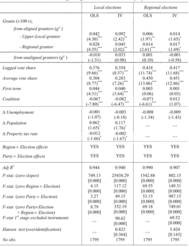
The results of the estimation of the effects of grants on votes for the incumbent are presented in Tables 2, 3 and 4. Table 2 presents the basic results, that is, the effect of total grants on the vote share of the incumbent at the local government and their effect when allowing for a differential effect of grants coming from aligned or unaligned grantors. Table 3 reports the same results for the vote share at the regional government. In both tables, the first two columns show the OLS results and then the Instrumental Variable (IV) ones. Table 4 presents the results when allowing for a differential effect of grants depending on the grantee layer of government (Regional or

Upper-Local). All tables estimate the linear version of the vote equation (5b), and use a limited set of controls. A discussion of the estimation of the non-linear version (5a) and the use of additional controls is included at the end of this section.

Table 2 shows, first, that total grants have a positive and significant effect on the incumbent’s vote share at the local elections, result that does not hold when using IV. Second the results point out that the effect of grants is significantly different depending on whether they come from aligned or unaligned governments. Concretely, the OLS estimators conclude that grants

from aligned governments, , have a positive and significant impact on the incumbent’s vote share at the local election while those from unaligned governments, , do not have any impact on the vote. These results hold in the case of the IV using average grants as instruments. The first-stage F-statistic of the excluded instruments suggest that the set of instruments used are jointly highly significant predictors in the first stage (they are much bigger than the threshold proposed by Stock and Yogo, 2003), and thus, they are not weak. Moreover, the value of the Hansen overidentification test indicates that the instruments are not correlated with the error term. These tests corroborate the validity of the instruments. We perform the regression based Hausman endogeneity test (Wooldridge, 2002), which corroborates that there is a problem of endogeneity. The IV coefficients are higher than the OLS. Thus, the OLS estimates seem to be biased downwards.

aL Jt g uL Jt g

Table 2. Effects of grants on the vote share of parties

in the Local government at the Local elections

OLS IV

[1] [2] [3] [4] [5]

Grants (×100 є),

total grants _(2.71)0.013 *** -.- 0.016 _{(0.72) (0.57)} 0.013 -.-

from aligned grantors (ga_{) -.-} 0.032

(6.26)*** -.- -.- _(2.37)0.074 **

from unaligned grantors (gu_{) -.-} -0.010

(-1.48) -.- -.- (0.91) 0.031

Lagged vote share 0.378

(9.61)*** _(9.72)0.378 *** _(9.14)0.377 *** _(9.16)0.378 *** _(8.62)0.354 ***

Average vote share 0.307

(8.78)*** _(8.77)0.304 *** _(8.49)0.307 *** _(8.54)0.307 *** _(7.48)0.287 *** First term 0.041 (4.00)*** _(4.32)0.044 *** _(3.95)0.041 *** _(3.98)0.041 *** _(3.98)0.040 *** Coalition -0.064 (-7.21)*** _(-7.78)-0.068 *** _(-5.69)-0.065 *** _(-5.60)-0.064 *** _(-6.37)-0.080 *** Δ Unemployment -0.005 (-1.03) (-1.07) -0.001 -0.005 (-1.01) (-0.91) -0.005 (-1.13) -0.019 ΔPopulation 0.059 (1.69)* _(1.65)0.060 * _(1.68)0.063 * _(1.65)0.058 * _(1.77)0.118 *

ΔProperty tax rate -0.014

(-1.67)* _(-1.68)-0.019 * _(-1.66)-0.019 * _(-1.66)-0.014 * _(-1.69)-0.002 *

Region × Election effects YES YES YES YES YES

Party × Election effects YES YES YES YES YES

Adj R2 _{0.943 0.944 0.943 0.943 0.941} F-stat. (zero slopes) 678.64

[0.000] [0.000] 795.85 10322.52 [0.000] 10439.27 [0.000] 26244.54 [0.000]

F-stat. (zero Region × Election) 3.09

[0.000] [0.000] 3.42 [0.000] 108.40 [0.000] 108.25 [0.000] 105.21

F-stat (zero Party × Election) 2.77

[0.000] [0.000] 2.50 [0.000] 49.47 [0.000] 49.09 [0.000] 47.34

F-stat (zero Party × Election

+ Region × Election) 8.39 [0.000] 8.50 [0.000] 530.98 [0.000] 354.59 [0.000] 343.87 [0.000]

F-stat 1st _{stage excluded}

instruments -.- -.- [0.000] 39.04 [0.000] 21.65 [0.000] 131.05 Hansen test (overidentification) -.- -.- -.- 0.750 [0.386] 1.715 [0.424]

Hausman test (OLS IV) ≠ -.- -.- 0.89

(2.01)** _(2.04)0.87 ** _[0.039] 3.25

No obs. 1795 1795 1795 1795 1795 Notes: (1) t statistics are shown in parenthesis and p-values in brackets; *, ** & ***: significantly different from zero at the 90%, 95% and 99% levels; (2) Robust standard errors; (3) Dependent variable is the vote share of the party/parties in the local government in the local elections; (4) Hansen test for instrument validity, distributed as a χ2

( )

n with n = number of over-identifying restrictions (p-value in brackets). (5): The Hausman test is based on the residuals of the first stage regression. When there is only one instrument, we report the estimated coefficient of the residuals, otherwise the F-test of joint significance is reported. (6) Instruments used: [3]:

g

; [4]: gL(UL)_{, g}L_{(R); [5] g}aL_{(UL), g}uL_(UL), ,gaL(R) _guL_(R)

Table 3. Effects of grants on the vote share of parties

in the Regional government at the Regional elections

OLS IV

[1] [2] [3] [4] [5]

Grants (×100 є),

total grants _(2.08)0.004 ** -.- _(0.75) 0.004 _(0.81) 0.004 -.-

from aligned grantors (ga_{) -.-} 0.008

(3.35) **

-.- _-.- 0.009

(1.68)*

from unaligned grantors (gu_{) -.-} 0.001

(0.09) -.- -.- (-0.25) -0.001

Lagged vote share 0.428

(12.05)*** _(11.90)0.420 *** _(12.10) 0.428 _(12.12)0.428 *** _(11.72)0.417 ***

Average vote share 0.453

(13.08)*** _(13.07)0.449 *** _(13.11) 0.453 _(13.09)0.453 *** _(13.15)0.447 *** First term 0.001 (0.19) (0.14) 0.001 (0.19) 0.001 (0.19) 0.001 (0.12) 0.001 Coalition -0.063 (-5.69)*** -0.068 (-6.26) *** -0.053 _{(6.26) (-8.27)}-0.086 *** _(-6.01) -0.056 Δ Unemployment -0.006 (-1.29) (-1.39) -0.008 (-1.28) -0.007 (-1.27) -0.007 (-1.40) -0.008

Region × Election effects YES YES YES YES YES

Party × Election effects YES YES YES YES YES

Adj R2 _{0.990 0.990 0.990 0.990 0.990} F-stat. (zero slopes) 1789.02

[0.000] 1452.33 [0.000] 3901.22 [0.000] 3987.24 [0.000] 2157.44 [0.000]

F-stat. (zero Region × Election) 56.85

[0.000] [0.000] 61.45 [0.000] 889.90 [0.000] 890.11 [0.000] 731.61

F-stat

(zero Party × Election)

50.89 [0.000] 40.40 [0.000] 164.91 [0.000] 165.13 [0.000] 120.22 [0.000]

F-stat (zero Party×Election + Region × Election)

49.79

[0.000] [0.000] 50.56 1033.35 [0.000] 1034.01 [0.000] 1057.78 [0.000]

F-stat 1st _{stage excluded}

instruments -.- -.- [0.000] 129.90 [0.000] 66.06 [0.000]] 128.49

Hansen test (overidentification) _{-.- -.- -.-} 0.401

[0.526] [0.558] 0.342

Hausman test (OLS ≠IV) 0.47

(1.02) (1.03) 0.48 [0.375] 0.983

No obs. 1795 1795 1795 1795 1795

Notes: (1) See Table 2. (2): Instruments used: [4]: gR(UL)_{, g}R_{(R); [5]: , g}aR_{(R) g}aR_(UL), )

(R UL guR ₊