How Much Can We Learn from International Comparisons of Intergenerational Mobility?

CEE DP 111

How Much Can We Learn From International

Comparisons Of Intergenerational Mobility?

Jo Blanden

November 2009

Published by

Centre for the Economics of Education London School of Economics

Houghton Street London WC2A 2AE

© Jo Blanden, submitted September 2009 November 2009 of publication

The Centre for the Economics of Education is an independent research centre funded by the Department for Children, Schools and Families. The views expressed in this work are those of the author and do not reflect the views of the DCSF. All errors and omissions remain the authors.

How Much Can We Learn From International

Comparisons Of Intergenerational Mobility?

Jo Blanden

1. Introduction 1

2. Measures and Concepts 2

Income mobility 3

Socio-economic mobility and social class fluidity 7

Educational persistence across generations 11

Conceptual links across the measures 12

3. Is There a Consensus? 14

Income mobility 14

Social status and class fluidity 16

Educational persistence across generations 18

What are the similarities and differences? How can they be explained 19

Aside on changes over time 20

4. Can We Explain The Patterns? 22

Cross sectional income inequality 23

Educational investment 26 Returns to education 27 5. Conclusions 28 References 30 Tables 34 Figures 39 Appendix 46

Acknowledgments

Jo Blanden is a Lecturer at the Department of Economics, University of Surrey, a Research Associate at the Centre for Economic Performance, London School of Economics, and a CEE Associate.

The author would like to thank Harry Ganzeboom, Richard Breen and Kevin Denny for generously sharing their data. She is also grateful to Cetin Salih for research assistance and to Anders Björklund, Christopher Jencks, Paul Gregg and Robin Naylor for extremely helpful comments. This paper is based on work commissioned by the Sutton Trust and the Carnegie Corporation of New York and was first presented at their June 2008 conference ‘Social Mobility and Education’.

1

1 Introduction

Intergenerational mobility is concerned with the relationship between the socio-economic status of parents and the socio-economic outcomes of their children as adults. This can be measured in a variety of ways, by income and earnings, social class or status, or education. If an individual‟s income/social class/education is strongly related to his or her parental background, this means that a child from a poor family is unlikely to escape his or her start in life and consequently inequality will perpetuate. This has implications for economic efficiency if the talents of those from poorer families are under-developed or not fully utilized, as those from poorer backgrounds will not live up to their productive potential.

Most people would agree that equality of opportunity is an important goal; nonetheless it is difficult to imagine a world with no link between outcomes across generations. Genetic transmissions alone are likely to lead to a positive association between the educational achievements, career prospects and earning power of parents and children, while learning within the family will lead to children from better-off families being better equipped to succeed. Hence the policy implications of the study of intergenerational mobility are unclear. If intergenerational income inequality is solely a consequence of the automatic transmissions of ability and other attributes within the family, its reduction would require strong intervention by the state, and might lead to inefficiency. Our understanding of this can be improved by making comparisons of the levels of intergenerational mobility across countries. With comparisons in hand, it is possible to assess mobility as „relatively weak‟ and „relatively strong‟, and then begin to consider potential explanations for differences in intergenerational mobility.

The first task in this paper is to summarise the literature on the relative strength of intergenerational mobility across different countries. In contrast to most other summaries, work on income, social class, social status and education will all be considered with observations of mobility included from 65 countries. If our question of interest is „How does the importance of the influence of parental background for children‟s outcomes differ across countries?‟ it does not seem reasonable to concentrate only on one measure of background and outcome. In addition we know there is a great deal of uncertainty about comparisons made on the basis of the income mobility literature (as highlighted in Björklund and Jäntti,

2

2008). It is therefore helpful to look at how estimates compare across different literatures. In doing so, we consider methodological issues carefully and select our „preferred estimates‟ for each measurement approach to represent the most comparable picture of mobility across countries.

We find that the different measures used tend to be fairly well correlated, with South America and southern Europe having low mobility and the Nordic nations being rather more mobile. Measures of the association of social class across generations (social class fluidity) are the exception to this, with if anything, a negative relationship between the country rankings on these measures and others. We shall examine the possible reasons for this difference later in the paper.

In the second part of the paper we begin with a short review of the theoretical literature that seeks to model the determinants of intergenerational mobility within society. This includes income inequality, educational investment, and returns to education. Finally we take our preferred measures of mobility and correlate them with these variables paying particular attention to contrasting results from our measures of income, educational and occupational mobility. We find evidence that income, status and educational mobility are all related to inequality, education spending and the returns to education.

These descriptive correlations cannot be thought of as painting a picture of the causal relationships that drive intergenerational mobility. However, owing to the intense interest in the relationship between inequality and immobility, it seems worthwhile to explore the extent of our knowledge in this area. In the conclusions remarks are made about the policy implications of the results presented here and we are also careful to discuss the further evidence required to make more concrete suggestions about how public policy could be used to promote mobility.

2 Measures and Concepts

Before we can review the empirical literature on mobility we need to gain a solid understanding of the methodologies used by the different measurement approaches, and the

3

main data features that can influence the estimates obtained. This understanding is essential in making international comparisons, as an inconsistent measurement approach can lead to invalid inferences about the difference in mobility across countries. We begin by reviewing the key methodological issues that arise in obtaining estimates of income mobility, an issue that has achieved substantial attention in recent years. We then discuss the measures and concepts used when social status, class and education are used as outcome measures. In conclusion we provide a review of the relationship between measures based on different outcomes, this provides a framework to interpret differences in the country rankings provided by different measures.

Income mobility

Measures of intergenerational earnings and income mobility are based on estimation of  in the following model:

lnYichild   lnYiparents ageiparentsageichildi (1)

where ln child i

Y is the log of some measure of earnings or income for adult children, and ln parents

i

Y is the log of income or earnings for parents, i identifies the family to which parents and children belong and iis an error term.  is therefore the average elasticity of children‟s

income with respect to their parents‟ income.1

Hypothetically, 0 represents a case of complete mobility where the incomes of parents and children are completely unrelated, and  1 represents a case of complete immobility where the proportionate earnings advantage of parents is precisely mirrored in their children‟s generation. Estimates of  tend to lie between 0 and 1, implying that an initial income advantage will be wiped out over several generations.

1

This linear formation is common, but see Bratsberg et al (2007) for a discussion of how international comparisons are affected by allowing for nonlinear relationships in earnings across generations.

4

Intergenerational mobility can also be measured by the partial correlation of parents‟ and children‟s incomes. This adjusts for differences in income variance between the two generations. Mobility can be thought of as measured by 1-r.

parents child ln | lnY , lnY ln | =Corr ( ) parents child Y age Y age SD r SD   (2)

Economic mobility can be measured either through income or earnings; in reality, the literature is dominated by estimates of the elasticity of sons‟ earnings with respect to fathers‟ earnings. This means that the importance of non-labour income is not acknowledged, those without paid employment are dropped and that the experience of women as both mothers and daughters has been frequently neglected (Chadwick and Solon, 2002, is a notable exception regarding daughters). As this paper is seeking comparable measures of mobility we also focus on the earnings mobility of men, but this does not mean that other measures are uninteresting, and they certainly deserve more widespread attention.

Models of intergenerational persistence2 tend to imply that the measurement of intergenerational mobility should be based on the permanent income of parents and children; unfortunately in datasets where incomes of both generations are available they are often only short-term measures. Under classical measurement error assumptions3 it is straightforward to show that measurement error in the dependent variable (the child‟s income) will not bias the estimate of, although it will lead to a loss of precision and larger standard errors. As discussed by Solon (1992) and Zimmerman (1992), measurement error in the explanatory variable has more serious implications and will lead to inconsistent estimates of . Indeed, the estimated parameter,ˆ, will be an underestimate of the true, as shown in equation (3), where 2_y and 2

u

 are the variances of fathers‟ permanent income and the error, respectively.

2 2 2 ˆ lim y y u p        (3)

2 _{See Goldberger (1989) for a discussion of how inherited endowments lead to intergenerational persistence and}

Solon (2004) for a model based on parental investments. Both lead us to expect that permanent income is the relevant concept.

3

These assumptions are that the level of y_i is uncorrelated with the size of the measurement error, and that errors are uncorrelated across generations.

5 It is clear that the „signal to noise‟ ratio (

2

2 2

y y u



  ) is crucial to obtaining accurate estimates of intergenerational persistence. If the variance of the error contained in parents measured income is small compared to the true variance of permanent income, then ˆ will be close to

 and we will have a good estimate of intergenerational persistence.

One strategy for reducing the downward bias associated with measurement error is to average parental income over several periods to come closer to a measure of permanent income. Under the classical measurement error model there will be a fall in the attenuating factor as more periods of data are used to generate the average, as shown in equation (4). As T

approaches infinity,

2

u

T



will converge to zero and ˆwill approach the true value of .

2 2 2 ˆ lim y u y p T



 





Work by Mazumder (2005) has shown that Solon‟s approach to solving measurement error by averaging parental income over five years or so may not be sufficient to overcome measurement error as the observations used are generally too close together to be truly representative of lifecycle income.

This topic is taken up in a rigorous way by Haider and Solon (2006). The starting point of their article is that the classical measurement error formulation is inappropriate as the relationship between permanent income and current income varies through the lifecycle. 4 As described by Mincer (1974), age–earnings profiles are steeper for those with more human capital (higher permanent incomes). Hence, at young ages current income is low compared to permanent income for those with high permanent income, while at older ages current income is higher compared to permanent income for those with high permanent income.

4

Haider and Solon‟s paper has been followed up by Böhlmark and Lindquist (2006) using Swedish tax register data. The Swedish authors find that the broad patterns found for the US also hold in Sweden.

6

Haider and Solon (2006) show that with this type of measurement error the direction of the bias is determined by the age at which earnings are observed. In addition, and unlike the classical case, measurement error in the dependent variable (children‟s incomes) will have an impact. The data used for intergenerational mobility often focuses on young sons and older fathers. Haider and Solon show that this combination is likely to lead to downward bias through both the dependent variable and the explanatory variables, and possibly to substantial underestimation. To minimize the extent of measurement error, incomes for both generations should be taken at the point when they are most representative of permanent income. Haider and Solon (2006) estimate this to occur at around the age of 42. Reville‟s (1995) empirical results support Haider and Solon‟s hypotheses. He finds evidence that ˆ rises substantially with the age at which sons‟ earnings are observed, particularly between ages 27 and 31.

An alternative solution to the classical measurement error problem is to use instrumental variables (IV). A valid IV is correlated with fathers‟ permanent income but uncorrelated with measurement error. In addition it should not independently affect children‟s economic status. The obstacle to using instrumental variables in this context is that almost every variable that is correlated with parents‟ permanent income might also have an independent impact on sons‟ status. This leads to an unambiguous upward bias in IV estimates of intergenerational persistence, meaning that they tend to provide an upper bound on the true extent of intergenerational transmission in a country.

The standard measurement approach requires information parental incomes and then children‟s incomes twenty or thirty years down the line, this severely limits the number of countries for whom intergenerational mobility can be estimated. Björklund and Jäntti (1997) use a variation of the instrumental variables technique to overcome this problem for Sweden in a way that has become increasingly popular and has enabled a large expansion in the number of countries for which we have information on intergenerational income mobility.

The Two-Stage Instrumental Variable approach (TSIV) is used when researchers have matched information on sons‟ earnings and fathers‟ characteristics (such as education and occupation) but no information on fathers‟ earnings. Fathers‟ earnings during the child‟s teenage years are predicted using information on the relationship between earnings and education from other data. Sons‟ earnings were then regressed upon this prediction. Subject

7

to certain assumptions, this estimator will be upward biased in the same way as other IV estimators. As discussed by Ermisch and Nicoletti (2007) the extent of the bias will depend upon the degree to which the instruments are directly related to the child‟s income and the strength of their ability to predict father‟s earnings. The larger the R-squared in the first-stage regression the smaller the bias will be. More recently this approach has been extended to Italy (Mocetti, 2007, Piraino, 2007), France (LeFranc and Tannoy, 2005) and in the international comparison by Andrews and Leigh (forthcoming).

In making international comparisons of intergenerational income mobility it is therefore essential to take account of the issues highlighted above; the approach taken to measurement error and the age of the fathers and children when earnings are measured.

Socio-economic mobility and social class fluidity

Measuring mobility by the statistical association of income or earnings across generations is actually a rather recent literature, with the majority of breakthroughs occurring since 1990. Much more established is the measurement of mobility by the links between social class or occupational status of fathers and sons.

One advantage of measuring intergenerational mobility by class or occupation is that the data restrictions are much less stringent, retrospective information on father‟s occupation is not difficult to collect and does not require the investment in longitudinal data necessary for intergenerational income studies. We may also think that occupation, broadly defined, varies less over the lifecycle making age–related biases less problematic. However, the difficulty with making international comparisons of mobility in social class or occupation across generations is the need for the measures to be comparable. This is a huge undertaking and has led to some large scale international projects and considerable controversy within the sociology discipline.

One approach to measuring mobility taken by sociologists is to create an index of socio-economic status (SEI) associated with occupations, match this index to fathers‟ and sons‟ occupations and then associate this index across generations. Generally the index depends on a weighted contribution of the average income and education within an occupation (where

8

weightings are chosen to maximise the relationship between the index and the education and earnings of occupations). Ganzeboom and Treiman (1996, 2003) have worked extensively on applying this approach across countries and we discuss some of their results below. These socio-economic indices can be correlated across generations using similar approaches to those reviewed in the measurement of income mobility. The strength of these correlations can then be compared across countries. The raw correlations are often not the focus of papers; this data is more commonly used in structural models that distinguish the degree to which the child‟s education acts as a transmission mechanism for parent and child socio-economic status. Another approach, as in Ganzeboom and Treiman (2007), is to use the correlations as explanatory variables in a structural panel model which seeks to explain why intergenerational mobility varies across nations and time.

An alternative approach to measuring mobility is based on class. Class divisions are also based on occupation but are formed of broad occupational groupings, which are supposedly un-ordered. For example, a frequently used schema is based on Erikson et al (1979).

I + II Service class Professionals, administrators and managers; higher-grade technicians; supervisors of non-manual workers

III Routine non-manual workers

Routine non-manual employees in administration and commerce; sales personnel; other rank-and-file service workers

IVa + b Petty bourgeoisie

Small proprietors and artisans, etc., with and without employees

IVc Farmers Farmers, small holders and other self-empoyed workers in primary production V + VI Skilled

workers

Lower-grade technicians; supervisors of manual workers; skilled manual workers

VIIa Non-skilled workers

Semi- and unskilled manual workers (not in agriculture, etc.)

VIIb Agricultural labourers

Agricultural and other workers in primary production

As social class is not a continuous variable, the measurement of social class fluidity (as it is commonly called) is based on the analysis of two-way contingency tables which document the moves between classes across generations. Modelling the patterns of mobility in contingency tables is a more difficult enterprise than correlating continuous variables and a large literature has evolved on how this can best be achieved. The major difficulty stems

9

from the fact that structural class shifts between generations will necessarily force some families away from the diagonal; increasing the appearance of absolute mobility. As a consequence it is important to have a measure of relative mobility which is invariant to compositional changes across generations.

Relative mobility is defined in terms of the odds ratios. For a 2x2 contingency table this is

11 22

12 21

(F F )

F F



 where Fijis the frequency of observations in cellijwhere i and j index father and

son‟s classes respectively. Each set of four cells in the contingency table will generate an odds ratio, taken together these provide a complete description of the patterns of mobility in the data. Log linear models provide a more parsimonious way of describing the total pattern of mobility in a contingency table.

If we take as the dependent variable Fijthen this can be explained by a scaling parameter μ,

the influence of the origin class i, the influence of the destination class, jand the influence

of the association between origins and destinations for this particular cell, _ij. So that F_ij   _{i j ij}for all i and j.

If we take logs of this model it becomes linear

lnF_ij   _iOD_j _ijOD (5)

In this way the model is fully saturated by the inclusion of origin (superscript O), destination (superscript D) and full interaction effects (OD), so the frequencies in each cell will be predicted perfectly. In a model of perfect relative mobility the _ijODterms will be equal to zero. The aim of log linear modelling is to avoid including all the ijOD terms but still achieve

an acceptable fit for the model. The _ijODterms omitted depends on the particular pattern of mobility the researcher has in mind, models depicting different mobility schemes can be evaluated depending on how well they fit the observed data. For more detail on the precise nature of these models see Erikson and Goldthorpe (1992) or Breen (2004).

10

When a cross country approach is taken a third dimension is added to the model, k. If the researcher believes that association effects are common across countries the log linear model becomes.

lnFij   iODj kCikOCDCjk ijOD (6)

A way of measuring variations in fluidity across nations is to examine how well this model performs; if it provides a good fit then this indicates that variation in the extent of class associations across countries is limited. Models allowing variations in the extent of particular origin-destination effects across countries enable a more complex pattern of similarities and differences to be built up.

Erikson and Goldthorpe‟s book The Constant Flux compared the extent of class fluidity for a number of countries in the late 1960s and early 1970s. The study initially concentrated on Europe with England and Wales, France, Northern Ireland, Scotland, the Republic of Ireland, West Germany, Sweden, Poland, and Hungary all examined closely. Analysis was also added for Czechoslovakia, Italy, the Netherlands the United States, Australia, and Japan. More recently Breen (2004) has followed up this study with an analysis of 11 countries, with significant overlap with those included by Erikson and Goldthorpe, Breen‟s aim is to understand trends in mobility for these countries from the 1970s onwards.

The models estimated in both of these books produce a very large number of parameters, and a great deal of detail on changing mobility patterns. For the purpose of this summary we would benefit greatly from a single mobility parameter for each nation and point in time. Erikson and Goldthorpe‟s (1992) UniDiff model provides such a statistic.

lnF_ij   _iOD_j _kC _ikOC_jkDC_ijOD_kX_ij (7)

ij

X depicts some general pattern of mobility and the coefficientkindicates how the strength

of the association varies across countries. k is normalised to some baseline so that a

11

This has necessarily been a very brief introduction to measuring social class fluidity. However it should hopefully give some intuition about the processes involved in the complex world of log linear modelling, and give an idea of how these methods have been used to draw comparisons across countries.

Educational persistence across generations

An alternative measure of mobility is the extent to which parents and children‟s education are related. The literatures on intergenerational income and social class or status persistence emphasise the role of education as a transmission mechanism; it seems natural to measure this association directly.

As with occupation, information on educational achievements across generations is quite widely available. Once again there are difficulties in ensuring that education has the same meaning across countries. One approach is to measure education in years of schooling, assuming that the meaning of this variable is constant across nations and generations. In this case educational persistence can be measured using the intergenerational coefficient and correlation, similar to the approach used for income mobility.

children parents

i i i

YearsEd   YearsEd u

and Corr_YearsEdparents_{, YearsEd}child ( )

parents child YearsEd YearsEd SD SD   (8) (9)

Cross national comparisons and 50 year trends in the coefficient and correlation of years of schooling have recently been presented by Hertz et al (2007) for 42 nations. We will draw heavily on this work when we come to summarise the international findings.

The above approach assumes (as does the measurement of income mobility, as presented here) that the impact of years of education on the next generation is linear and monotonic. It seems unlikely that this will be true, and even more unlikely that this will be true in all countries. As an example, the structure of the UK schooling system means that it is inappropriate to estimate simple years of schooling effects here (Dearden et al, 2002). To

12

overcome this problem we might wish to consider education in terms of qualification levels. This is more demanding in terms of cross-national comparability. Chevalier et al (2009) use the UNESCO designed ISCED classification as the basis of the five-category coding of education to measure the intergenerational association of education in Europe and the US.

Using a categorical measure raises difficulties of the type faced in the social class fluidity literature: how can we measure associations in education across generations as successive generations become more educated? The approach taken to this question by Chevalier et al is to model the associations in education by two measures; the eigen value index which summarises the degree of mobility implicit in a transition matrix – how rapidly parental education origin is forgotten - and the Bartholomew index which computes the average number of categories moved between generations.5 Chevalier et al find a relatively weak correlation between these two measures. It seems that the modelling approach taken to education persistence matters. We will consider in more detail how different measures change country rankings in Section 3.

Conceptual links across the measures

Taking first the relationship between income and education measures of mobility. Recall the linear model of intergenerational income mobility (omitting age controls):

lnY_ikchildren _k_klnY_ikparents_ik (10)

where the subscript k indicates that the mobility relationship varies across countries. In each generation education has a return in the labour market so that

5

2

1

Eigen value index   

where 2 is the second largest eigen value, the largest eigen value of any transition matrix is one. If 2 is equal

to zero then the transition matrix equals to the limiting invariant matrix and corresponds to equality of opportunity.



f ij is the joint frequency in the i,jth cell of the transition index and the modulus of (i-j) is the number of changes

in education level made from one generation to the next. In essence it is summarizing how far the population is from the principal diagonal of the matrix.

13

1

lnY_kparent _k _kparentEd_ikparent v_ik

and lnY_ijchild _2k _kchildEd_ikchild u_ik.

(11) (12)

k

 is a linear measure of the persistence of education across generations. It can be easily be shown that the relationship between _k and _k is:

( , ) ₁ ( , ) ( , )

.

( ) ( ) ( )

ik ik ik

ik ik

child child parents

child

k ik ik ik

k

k parents k parents parents

k ik k

Cov Ed v Cov u Ed Cov u v

Var v Var Ed Var v

 

 

 

    (13)

The first term gives the relationship between intergenerational mobility in income and earnings if education were the only route for intergenerational transmission. In this case the relationship between the two would be moderated by the relative size of returns to education, if returns to education increase across generations then income persistence will be higher than educational persistence and vice versa. The second term is the impact of the relationship between parental income (orthogonal to education) and child‟s education while the third term is the other cross effect between parental education and the child‟s residual earnings. The final component shows the relationship across generations of those components of earnings/income that are independent of education. It is clear that while income and education persistence are likely to have a positive correlation there are many other components which will lead to this correlation being less than one. One important element of this is the extent to which parental income and education influence uik, which can be thought

of as the within-education inequality in income.

It is easy to see how the above equation could be modified to express the relationship between socio-economic status mobility and income mobility, with _kinstead indicating the association between status and the _k terms giving the income return to status. Björklund and Jäntti (2000) assert that differences in the extent of mobility by income and social class can be explained by the extent of inequality; the US is rather immobile on measures of income persistence, but rather more mobile in terms of class fluidity, the difference can be explained by the extent of income mobility, we shall return to this argument below. Blanden, Gregg and Macmillan (2008) make a similar argument about the relationship between social class

14

fluidity and income mobility in the UK; asserting that the transmission of income inequality within classes is essential to explaining differences in results across approaches.

3 Is There A Consensus?

Income mobility

The comparison of intergenerational income elasticities has become a reasonably well worn path, with studies by Solon (2002) Corak (2006) d‟Annio (2007) and Björklund and Jäntti (2008) all seeking to draw together the international evidence on mobility. The introduction to income mobility provided in Section 2 has outlined the crucial measurement issues which can cause estimates of income mobility to be biased. It is essential that the estimates of mobility chosen for different countries are similar in their approach to measurement error and the age at which income is measured for each generation. In addition, as income mobility may change over time it is important that comparisons are made for cohorts as close in birth date as possible. My preferred estimates are for cohorts born in the late 1950s or early 1960s and I consider the relationship between the earnings of fathers and sons.

The selected estimates are listed in Table 1. They are based on two techniques, OLS using a time average of fathers earnings (based on around 5 years of data) and TSIV where fathers‟ earnings are predicted on the basis of his other characteristics. As discussed in the methodology section, we would expect the TSIV estimates to be upward biased compared to those based on OLS. Here I follow Corak (2006) in scaling down the TSIV estimates to make them more comparable. This is done on the basis of the bias detected in Solon (1992) and Björklund and Jäntti (1997), in both cases the OLS estimates based on the US PSID are smaller than those based on IV approaches by a factor of 0.75. This is only a rough estimate of the likely bias in other countries, but seems preferable to leaving the estimates uncorrected.

For the UK Dearden, Machin and Reed (1997) uses IV approaches for the 1958 cohort to get an estimate of 0.58, this is scaled down to give 0.435, however this is extremely high compared to the estimate from the British Household Panel Study given in Ermisch and Nicoletti (2007), which is 0.29 for the relevant cohort. In order to recognise the fact that

15

„There is a lot of uncertainty about the UK‟ (Björklund and Jäntti, 2008) we average the two estimates to give our preferred figure. This is in contrast to other surveys; Solon (2002) and Corak (2002) rely exclusively on Dearden, Machin and Reed, while Björklund and Jäntti (2008) prefer Ermisch and Nicoletti‟s estimate.

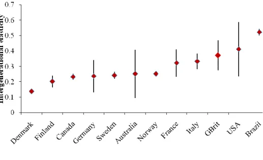
Figure 1 provides a visual comparison of our preferred estimates of intergenerational income persistence. There are 12 countries represented, and as we shall see this is small compared to the number of countries for which there is information on education and status mobility. While it is tempting to immediately form the estimates into a „league table‟ we must pay attention to the size of the standard errors; these are large in many cases. Although it does seem to be the case that the Nordic nations have higher mobility, it is impossible to statistically distinguish the estimates for Sweden and the US. The appropriate ranking at the top end is difficult with large standard errors on the Australian, French, British and US estimates making it unclear how these countries should be ranked.

Brazil sticks out clearly at the top of the graph as having low mobility (which is quite precisely measured). This is our first evidence that they may be stark differences between estimates of mobility for developed and developing countries or across different regions of the world. Grawe (2004) considers mobility for a broader range of countries and finds persistence in Ecuador, in particular, to be far higher than any estimate for developed countries.

The study by Andrews and Leigh (forthcoming) provides estimates of mobility for 15 nations using a TSIV methodology with the explicit purpose of considering the relationship between mobility and inequality. In this study Andrews and Leigh report both intergenerational elasticities and correlations and we use these to supplement the picture painted in Figure 1 (few of the studies used in Table 1 also report correlations). Figure 2 shows the estimates of mobility from this study. The set of countries considered here is rather different from those in Figure 1, but there is some similarity in the ranking, Sweden, Canada and Germany are fairly mobile, and the South American country included, Chile, is highly immobile. There is however some changing of the ordering of countries with the US appearing slightly more mobile than Australia. Overall the figures in Figure 1 are preferred as they are based on an extensive literature review, but the information from Andrews and Leigh is a useful

16

robustness check providing information on more countries as well as measures of the intergenerational correlation. 6

Social status and class fluidity

Erikson and Goldthorpe (1992) provided an analysis of international comparisons of social class fluidity for the 1970s which has been recently updated in Breen (2004). The discussion of cross national similarities and differences in both Erikson and Goldthorpe (1992) and Breen (2004) is incredibly rich with a great deal of detail concerning the extent of mobility between particular classes.

Both studies also provide summary measures from the UniDiff model. These are included here in Figures 3 and 4. In the earlier study the average extent of mobility is normed to 0 while in Breen this normalisation is on 1. Our discussion of mobility so far has indicated notable differences between the Nordic nations and the US. As discussed by Björklund and Jäntti (2000) and revealed clearly in Figure 3 Sweden and US both appear to be rather high mobility nations when measured by social class in the 1970s. Germany has the least mobility in Breen (2004) and is among the lower mobility nations in Erikson and Goldthorpe (the sample of comparator countries is rather different), this is in contrast to our earlier results for income mobility for which Germany looks rather mobile. It should be noted that Erikson and Goldthorpe consider mobility for all sons in the 1970s, they will be including those born several decades before the 1960s; the main cohort considered for our summary measure of income mobility.

Breen updates the UniDiff model up to the 1990s, again selecting all adult males rather than a particular cohort. His results for the most recent time period are given in the final bar for each country in Figure 4. Once again we see striking differences between these results and those for income mobility, the least mobile country is Germany, and Poland is found to be one of the most mobile countries (in contrast Andrews and Leigh found it to have high income persistence). There are clearly some striking differences between international

6 _{The TSIV estimations in this paper are based on finely graded occupation. This means that the estimates}

obtained will lie somewhere between a pure income and a social status approach. Differences in rankings between Figures 1 and 2 can be interpreted in this light.

17

rankings of mobility depending on whether they are measured by income or social class. Some of these differences might be explicable by dramatic changes in mobility across cohorts (this might be the case for Poland) but it seems unlikely that they are all explained by this. One plausible explanation is that within social class, differences in income mobility are sufficiently large such that the two measures do not correspond. We might anticipate such an effect with such large class groupings. An alternative is that the class groupings used are not equally good at representing the true occupational structure across nations. We next turn to results for status mobility to see if these results also differ to such an extent.

Ganzeboom and Treiman (2007a and 2007b) have been kind enough to supply some results from their latest international comparison of status mobility. Their results are based on pooling useable observations on fathers‟ and sons‟ occupations from a variety of data sources and then attempting to understand why correlations vary according by context, where a context is defined by the interaction of country, labour market entry cohort (5 year categoeis) and years of experience (10 year categories). As the authors have supplied the correlations by context we need to decide which is most comparable with the other results presented here. Our selected group are those entering the labour market in 1980-1985, whose occupations are observed with between 10 and 20 years of experience. Year of entry into the labour market is based on the year that education ended, so these cohorts were born between the mid-1950s and the late-1960s.

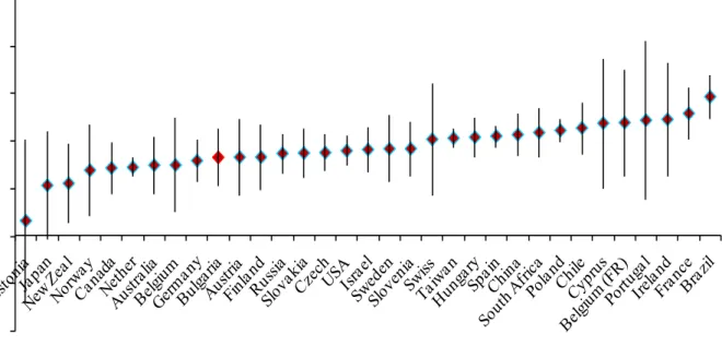
Figure 5 provides a graph of the correlations between fathers‟ International Socio-Economic Index (ISEI) and sons‟ ISEI across countries. This provides information on a larger number of countries than we have seen so far. As far as we can say, it seems that many of the patterns in the intergenerational income mobility literature are repeated: Norway and Canada are among the highest mobility countries while Brazil, France, Chile and Poland (along with other less developed nations and southern European countries) are at the other end of the scale. Once again the US and Sweden are close together in the centre of the graph. Germany‟s position is more similar to its ranking by income mobility than class fluidity. As with the income elasticities presented in Figure 1, it is noticeable that the standard errors are large, giving few clear differences between countries.

There are caveats to be borne in mind when using these results. It seems natural to consider the extent to which estimates vary within nations; how would the picture in Figure 5 look if

18

we had chosen a different cohort or experience level? Different measures for the same country are generally positively related but the correlation is not high (about .3 for the same cohort at different experience levels). It seems likely that this weak association is attributable to the mix of different data sources used to estimate the correlations, unfortunately the data provided does not allow us to assess the influence of the source dataset on the results. The dependence of the year at labour market entry on the education level means that the year of birth is negatively correlated with the time spent in education for our selected sample, a feature not present in the other estimating samples we use.

A limited review of the extensive social class and status mobility literature indicates that, despite the limitations of the estimates used here, measures of status appear to be capturing something similar to measures of income mobility while measures of class are more divergent. Notable exceptions to this statement are the US and Sweden which appear at opposite ends of the intergenerational income mobility ranking but are found rather more close together in the middle of the distribution when intergenerational associations are measured by status or class. Germany appears to be more immobile by class or status measures than it does by income. We will attempt an explanation of these findings at the end of this section after considering the findings from intergenerational correlations in education.

Educational persistence across generations

As mentioned in our discussion of measurement, intergenerational educational associations can be computed either for years of education or education categories. Hertz et al (2007) measure association using years of education for a large number of countries and results for both the regression coefficient and correlation are provided in Table 2. The first striking result is that Hertz et al (2007) find confirmation of two results found for a more limited range of countries elsewhere; that intergenerational mobility is low in South America and high in the Nordic nations. Of the western nations, Italy and the US are the least mobile as measured by the intergenerational correlation in years of education. Great Britain is immobile when measured by the intergenerational elasticity but mobile when measured by the correlation. This difference stems from the low variability in years of schooling for parents in the sample (almost everyone left at the end of compulsory schooling) and indicates

19

a limitation of measuring mobility in this way. For all countries in the sample the correlation between the coefficient and correlation is 0.40.

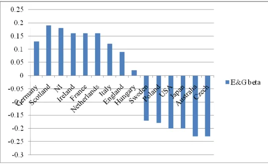
Results for the Bartholomew index and Eigen values from Chevalier et al (2009) are provided in Table 3, listed here from least to most mobile by the Eigen-value. The order of nations is becoming familiar, with Germany, Chile and Poland at the top and the Nordic countries at the bottom. In this ranking Great Britain appears to be rather immobile, less so than Italy. In contrast the US is in the lower-middle part of the Table in this case only a little less mobile than the Nordic nations. In the remainder of our analysis we take the eigen value as our preferred measure of categorical education persistence, because the meaning of this measure in terms of the speed at which origins are forgotten seems to have more in common with the intergenerational income parameters than the Bartholomex index does. We use (1-eigen value) as this has the same implication - higher equals less mobility – as the other measures we have used so far.

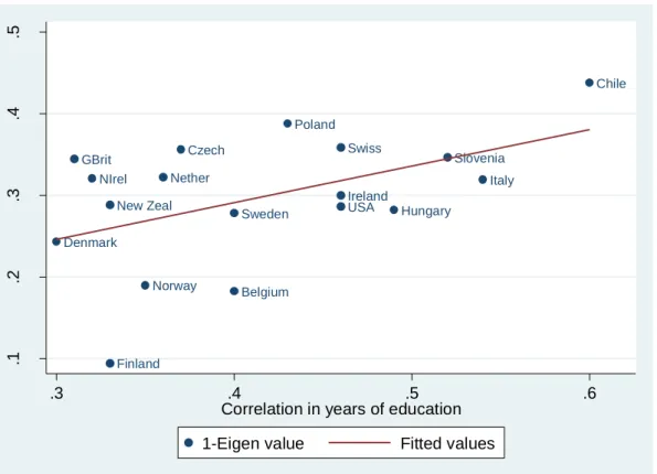
To complete this section we consider the relationship between our two preferred measures of educational mobility, Hertz et al‟s correlation and 1-eigen value. A scatter plot of these two measures is found in Figure 6 and shows a fairly strong relationship between the two measures with a correlation of 0.5.

What are the similarities and differences? How can they be explained?

Throughout our selected summaries of the income, social class, status and education mobility literature, we have made comments on the ways in which the measures and rankings have pointed towards common patterns of mobility across nations and we have also drawn attention to stark differences in the implications of these literatures for particular countries.

In terms of similarities; South America, other developing nations, southern European nations and France tend to have rather limited mobility by all measures. The Nordic countries tend to have rather high mobility, although Sweden often appears to be less mobile than the other nations. There are also some notable differences between the measures. Generally speaking the US appears rather immobile by income and education measures while appearing much more mobile by measures of social class and status. Germany in contrast is rather mobile on

20

income but immobile for social class and education. The UK tends to be towards the immobile end of the spectrum on all measures.

In Section 2.4 we considered the links between the different notions of intergenerational mobility. These suggest some ways in which differences in results can be reconciled. As discussed in Björklund and Jäntti (2000) the differing results for the US are explicable by the fact that it is a high inequality nation, with a large amount of income variation within the broad social class measures. An explanation of the differences for Germany might be lower inequalities within class and weaker income returns to class and education. An alternative explanation for the outlying results for social class may be that the ability of Erikson and Goldthorpe‟s measure to describing the class structure varies across countries. This might be because differences between the classes (in terms of some underlying latent variable) differs. Ganzeboom and Treiman‟s approach should mitigate this to some extent as their index is explicitly scaled by income and education, however, as we have seen, the ISEI correlations that are currently available have their own problems in terms of robustness and comparability with other measures.

Table 4 provides an overall picture of the similarities and differences in the different measures by listing the correlation coefficients between them. In many cases the sample of countries used do not overlap very much resulting in rather small sample sizes, we therefore would not want to over-emphasise these results. One thing that is very clear is that while the measures of income, education and status links across generations tend to be positively correlated this is not the case for the measures of social class fluidity. It appears that these constructs are tapping into rather different mechanisms; we therefore do not include them in the rest of our analysis. Note that the two measures of social class fluidity are closely linked for the eight countries that have both available; this is true even though they relate to different periods.

Aside on changes over time

Our analysis so far has concentrated on comparing intergenerational mobility across countries for people currently in the labour market, born around 1960. While we can learn a lot from these measures they are obviously not a measure of mobility for those growing up in the

21

policy environment of the 2000s. Before proceeding, it therefore seems worthwhile to make some comments about the changes in mobility over time as measured by the four different measures and to consider the picture for children growing up today.

The results for the UK included in this paper refer to the period before the fall in intergenerational mobility found in Blanden et al (2005). This picture of a relatively unfavourable trend in mobility for the UK is also confirmed by Hertz et al (2007) for educational correlations which show an increase over a fifty year period.The latest evidence for the UK indicates that this fall in mobility has not continued among cohorts born from the mid 1980s onwards (Blanden and Machin, 2008).

Changes in intergenerational income mobility in the US have been considered quite extensively in recent years. Corcoran (2001), Fertig (2003/4) and Mayer and Lopoo (2005) all find a fall in intergenerational persistence while studies by Levine and Mazumder (2002) and Lee and Solon (2006) have more ambiguous findings. Aaronson and Mazumder (2007) find a rise in the intergenerational elasticity from 1980 to 2000 but no change in the intergenerational income correlation. Results for the US on educational mobility in Hertz et al (2007) show a rise in the intergenerational correlation of education.

In the study we draw on for the French results in Table 1, Lefranc and Tannoy (2005) explore changes across cohorts considering cohorts born 1937–47, 1945–55 and 1963–73. The last two groups may be seen as broadly comparable with those considered for the UK but in contrast to the UK results, their estimates of remain very steady across all three cohorts. Two studies of changes over time have been carried out for Nordic countries. The analysis presented in Bratberg et al. (2005) for Norway compares intergenerational elasticities estimated for the 1950 and 1960 cohorts when they were in their early 30s, cohorts which slightly predate those used in Blanden et al.‟s (2005) analysis. The authors find a slight decline in intergenerational associations for sons. Österbacka (2004) considers this question for Finland and finds no clear trend.

In light of the concern that changes in mobility over time might lead to differences in the international ranking of countries for children growing up today, Figure 7 taken from

22

Scheutz, Ursprung and Woessman (2005) shows the relationship between family background and test scores in TIMSS which seeks to measure the achievement of children in a comparative way across nations. It is noticeable that the US and UK (alongside Germany) appear to have rather strong relationships between family background and test scores among children growing up today.7 For cohorts not yet in the labour market, those in Germany, the UK and the US (alongside some developing and transition nations) appear to have the poorest prospects for mobility through education.

4 Can We Explain The Patterns?

This paper has so far provided a (selective) review of the literature on international comparisons of intergenerational mobility and found some common themes in the story presented by the different approaches. The next step is to try to explain the differences we find between nations. We first consider the theoretical perspectives that have been taken on this question before considering the empirical evidence.

Becker and Tomes (1986) provide the original economic model of intergenerational income mobility. The framework is based on the idea that parents make investments in their children, in a model where parents and children have perfect access to credit markets there will be no direct relationship between parental income and investments. Any relationship between incomes across generations will be driven entirely through the inheritance of characteristics rewarded in the labour market (labelled endowments). Public policy could have an important role in encouraging mobility through the school system (weakening the heritability of endowments) or by supporting higher education in cases where credit constraints are binding.

Solon (2004) builds on the Becker-Tomes framework and provides an economic model which explains intergenerational mobility as a function of parental and state investments in children. He shows that intergenerational income persistence will be higher if heritability (the genetic transmission of endowments) is higher, if the productivity of investment in education is

23

higher, if the returns to education are higher and if government investment in human capital is less progressive. Solon also shows that the same parameters are important for generating income inequality so that inequality and intergenerational persistence will tend to have a positive relationship.

We might also think of other more direct connections between inequality and mobility. If the distribution of income is wider in country A than country B children at the bottom may be relatively more disadvantaged in country A and will face greater barriers to upward movement. The desire to improve intergenerational mobility in the UK is in part behind the policy aim to eradicate child poverty. This paper can only begin to investigate the relationship between inequality/poverty and mobility we consider this an area ripe for further research.

The preceding discussion leads us to focus on two broad dimensions by which countries may differ and which may help to explain differences in the extent of mobility; inequality and the education system. In the remainder of the paper we shall correlate measures of inequality, public educational investment and private educational returns with the measures of mobility used so far.

Cross sectional income inequality

The relationship between mobility and inequality is of considerable interest. The American Dream is based on the hypothesis that cross sectional income inequalities can be offset by equality of opportunities, and that inequality should be less of a concern if there is a high level of mobility. If greater inequalities go hand-in-hand with fewer opportunities it is much more alarming. Our basic picture of Nordic countries at the top of the mobility ranking and South America at the bottom certainly points towards a negative correlation between the two, and Andrews and Leigh (2008) confirm this statistically. We check this for the countries we have here and experiment with using different measures of inequality and child poverty.

Our inequality measures are predominantly taken from the Luxembourg Income Study (LIS) which provides cross-nationally comparable estimates for a variety of measures of income inequality and child poverty. Led by the theoretical discussion above we would like to

24

consider inequality measured at two points, when the children were growing up and at the point when their adult outcomes are measured. As we have focused on children who were born around 1960 we would ideally require income inequality measures for the 1970s. The number of nations for whom inequality data is available in the LIS increases as we consider more recent years. We start with 1982, but for those countries where this is not available we use later years. We supplement this information with income inequality taken from the World Bank dataset based on Deininger and Squire (1996), which is also used by Andrews and Leigh (2008). This provides inequality measures for the late 1970s/early 1980s. Information on inequality in the adult years is available for 1995 and 2000 from the LIS.8

Table 5 provides the correlations between income inequality and our measures of intergenerational immobility. In all cases these are positive. Nations with high inequality tend to have high persistence in social status for all of our measures. Although we would not want to make too much of it owing to the small sample sizes used there are some interesting variations in the strength of these correlations.

Taking the Table as a whole the majority of correlations are quite large, at over 0.5, indicating a strong positive relationship between inequality and intergenerational mobility. There are some interesting differences across the measures, with our preferred income beta tending to be most strongly correlated with income inequality in adulthood while the other measures show a larger association with inequality levels earlier in the relevant cohort‟s life. This is not surprising as the income beta is most likely to pick up the influence of labour market returns while the other measures are less influenced by this and dependent on the opportunities available to the cohort as young people.

It is also notable that we see the income elasticity from Andrews and Leigh is more closely related to inequality than is the case for their correlation measure. Aaronson and Mazumder (2007) find that as inequality increased for the US from 1980 onwards the income elasticity rose while the income correlation remained constant.

8 _{An alternative source of inequality information is the share of top incomes, as brought together by Leigh}

(2007b); unfortunately these are only available for seven of the countries for which we have information on intergenerational income mobility.

25

There is no consistent evidence that the child poverty measure is more strongly correlated with immobility than are the general measures of inequality. Indeed, rather counter-intuitively it appears that the measures related to income inequality at the top of the distribution (the 90-50 ratio) has a stronger association with immobility than the other measures of income inequality, although the size of these differences is too small for us to discriminate such patterns with any certainty.

Our theoretical discussion of the relationship between inequality and mobility highlighted two possible mechanisms. One was that inequality and immobility tend to be generated by the same factors and that we would therefore expect the two to be correlated at the end of the process (when the second-generation are adults). The second is that inequality in childhood inhibits equality of opportunity. The limited evidence presented in Table 5 indicates that it is inequality in childhood that matters for the non-income measures while our preferred income mobility estimates are also very strongly correlated with inequality in adulthood. This is because intergenerational income mobility is influenced by the adult returns to characteristics such as education and occupation.

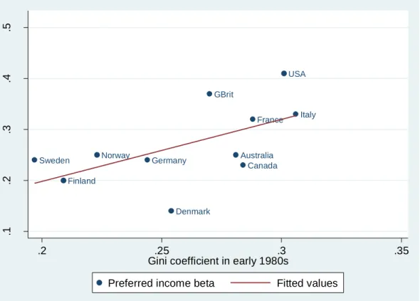
Figures 8a and 8b shows the relationship between the preferred beta and the gini-coefficient in the early 1980s and in 1995. This reveals why the correlation with income mobility is stronger for inequality measured in 1995 than in the early 1980s. The two key observations seem to be Denmark, for which inequality fell by about an eighth to match the low level of intergenerational persistence, and the UK where inequality rose by 25 percent over the period. One should be cautious in interpreting these results as a consequence, especially given the large standard error on the British estimate of beta.

This preliminary analysis of the relationship between inequality and mobility has indicated several interesting pieces of evidence. 1) There is the expected relationship between inequality and mobility. 2) The relationship between mobility and poverty is not driving this, inequality at the top is important as well. 3) Inequality in childhood appears crucial for all measures, but inequality in adulthood also matters for our preferred measure of income persistence.

26 Educational investment

Solon (2004) highlights the importance of the progressivity of educational expenditure as a factor leading to greater mobility. We are rather limited in the way we can operationalise this concept, the OECD Education at a Glance provides a large amount of information on education spending such as the proportion of spending coming from private and public sources, however this information is difficult to obtain for the 1970s. Instead we use information from Barro and Lee‟s (1994) international panel dataset. This provides Government education spending as a proportion of GDP, for both total and recurring expenditures. This measure will certainly compound different aspects; the level of total spending relative to GDP, and the extent to which spending on the education is carried out by Government. We take average figures from 1965-1969 (the primary school years for the 1960 cohort) and 1970-1974 (the early secondary school years) and once again correlate these with our measures of mobility.

As we would expect, there is a negative relationship between education spending and intergenerational persistence. Those countries which devote more of their income to public spending on human capital investment tend to be more mobile. This correlation is slightly stronger with the income beta than with other measures, and these two variables are graphed in Figure 9. Interestingly Andrews and Leigh‟s correlation measure is more closely related to education spending than their elasticity is, so it is not the case that the previous result that elasticities correlate more strongly with inequality is replicated for all the explanators. Total education spending tends to be more closely related to mobility than recurring spending and there is no consistent pattern on the most important period of schooling, primary or secondary.

A possible explanation for the results is that education spending and inequality are picking up the same characteristics of nations. The correlation between the gini coefficient and education spending is in the region of -0.3 to -0.5. However some positive evidence comes from the status correlation measure; a regression of this on both the World Bank gini and educational expenditure in the 1970s gives a significant coefficient of the expected direction on both (although the coefficient on inequality is very small in magnitude). However, while this is indicative we do not really have enough data to robustly compare the influence of individual variables.

27 Returns to education

A further prediction from Solon is that income mobility will be weaker when the returns to education are larger. Recall the relationship between intergenerational income mobility in country k (_k) and the correlation in education across generations (_k). Clearly the return to education for the child has a positive relationship with the income _k. We might also suspect that k will have a positive link to the return to education as better educated parents

will have a greater incentive to invest their extra resources in their children‟s education if the return to this is higher.

( , ) 1 ( , ) ( , )

.

( ) ( ) ( )

ik ik ik

ik ik

child child parents

child

k ik ik ik

k

k parents k parents parents

k ik k

Cov Ed v Cov u Ed Cov u v

Var v Var Ed Var v

 

 

 

    (14)

Table 7 gives correlations between our mobility measures and the returns to education as listed in Psacharopoulos and Patrinos (2004). Once again the correlation is as expected. Two measures are used, the average return to a year of education and the return to higher education. The higher education measure is more strongly related to mobility than the average measure. This could be interpreted as being because higher education is the most important route for intergenerational persistence/mobility, but it may also be the case that the higher education return is subject to less measurement error across countries. Our predictions concerning the relative strength of correlations with different measures of mobility are also found to be accurate. Both measures of returns are found to be correlated more strongly with income mobility (all three measures of this) than with status or educational mobility. This is because income mobility is influenced by income returns through the final outcome (earnings) while educational mobility will only be influenced by returns because of the incentives to invest.

Figure 10 shows a scatter-plot of the relationship between higher education returns and the income beta. This graph gives further evidence as to why the income and education rankings differ for Germany; Germany has a low return to education compared with Italy and France.