Turkish Economic Review
www.kspjournals.org
Volume 4 September 2017 Issue 3
What determines the growth of services sector in
Pakistan? A comparison of ARDL bound testing and
time varying parametric estimation with general to
specific approach
By
Muhammad AJMAIR
a†Khadim HUSSAIN
abSabahat AKRAM
ac& Ambreen ZEB
dAbstract. This empirical study followed time varying parametric approach (Kalman Filter) and auto regression distributed lag (ARDL) with general to specific approach to find out relevant macroeconomic determinants of Pakistan’s services sector’s growth. To our best of knowledge, no author has made such study that employed these estimation techniques to find out determinants of services sector growth in Pakistan while employing general to specific approach. Current study bridges this gap. Annual data was taken from World Development Indicators (2014) during period 1976-2014. Main findings of the study are that rolling regression estimates of explanatory variables justify the use of Kalman filtering approach. Results show that inflation has negative effect on services sector output growth in case of TVP approach. This result does match with ARDL results. Net foreign direct investment has positive and significant effect on services sector output growth in both techniques of estimation. Gross national expenditures with positive effect are the relevant significant determinants of services sector output growth at five percent significance level in case of TVP approach while relationship was insignificant in case of ARDL estimation. Impact of remittances received on services sector growth is negative in case of time varying parametric approach. This result is different from ARDL results where relationship is positive and significant at five percent level of significance. All the one step ahead state vectors confirmed the stability of models in case of time varying parametric approach. Cumulative sum of recursive residuals (CUSUM) and cumulative sum of recursive residuals square (CUSUMQ) also confirmed the stability of results of auto regression distributed lag. Based on these empirical findings, we conclude that government should focus on service sector growth augmenting factors while formulating any policy relevant to the concerned sector.
Keywords. Services sector, Kalman filter, Rolling regression. JEL. C22, O11, O40.
1. Introduction
gricultural, industrial and services sectors are the major components of economic growth of Pakistan. In the very beginning years of Pakistan Independence, contribution of agriculture sector in economic growth was aa†
Department of Economics, Mirpur University of Science & Technology, Mirpur, AJK, Pakistan. . +92 300 621 5532
b
Department of Economics, Mirpur University of Science & Technology, Mirpur, AJK, Pakistan. . [email protected]
c
Director Planning & Development/Chairperson Department of Economics, University of Management Sciences & Information Technology, Kotli, AJK, Pakistan.
d
Department of Economics , University of Sindh, Jamshoro, Pakistan. . [email protected]
more than industrial and services sectors. With the passage of time, contribution of services sector has increased. Services sector’s contribution to economic growth is 58.8 percent, industrial sector has 20.30 percent and agricultural sector has 20.90 percent share (Economic Survey of Pakistan, 2014-15). Both industrial and services sector contribution adds up to approximately 80 percent of overall GDP growth of the country. In such a situation, it is necessary to find out the relevant determinants of services sector growth in Pakistan. It will make capable us to recommend policy measures to boost up services sector for better economic growth of the country. No author has made such study that could collect a number of variables from existing empirical literature and capture the effect of structural changes on relevant determinants of services sector growth in Pakistan while employing general to specific approach. Current study will bridge this gap.
Over the time, the structure of any economy changes and the constancy of estimated parameters are affected significantly by these structural changes. According to , Engle & Granger (1987), Philips & Perron (1988) and Johanson & Juselius (1990) the fixed parametric approaches like auto regressive distributed lag (ARDL) don’t take into account impact of structural changes on estimated constant parameters. It is compulsory to employ a time varying parameter approach to evaluate the impact of structural changes on constant estimated parameters (Gilal & Chandio, 2013). Kalman Filter is applied as a time varying parametric approach. Thamae et al. (2015) preferred Kalman filter (1960, 1963) estimation strategy than other conventional method of estimation due to following advantages. First, Kalman Filter is an ideal approach as the impact of variables used changes with time (Slade, 1989). Second, Kalman filter is considered to be better than the least squares methods particularly when the parameters are not stable (Morisson & Pike, 1977). Third, this approach of estimation is prognostic and adaptive and it can be applied without checking the stationarity of variables (Inglesi, 2011).
To justify the usage of time-varying parameter approach rolling regression methodology was applied. We used annual data for the sake of reduction variation and serial correlation in selected data. Annual data was also used by authors in different studies of (Moosa, 1997; Viren, 2001). Parametric rolling regression was estimated through ordinary least square method during period 1976–2014. K1
was set to 12 year. Same process was adopted by authors in their studies (Moosa, 1997;
Gilal & Chandio, 2013). The Kalman filter (1960) is employed recursively by time to find out forecasts and variance of forecast. The Kalman filter is crucial because it may be employed in real time. That is, as each value of the annual data is noticed the forecast for the next observation can be calculated (Hyndman & Snyder, 2016). Organization of study is as the section two includes literature review, section three includes methodology: data, model and estimation technique. Section four discusses results, fifth section concludes the study.
2. Literature review
Gross domestic product is sum of the value of products produced by three sectors namely agriculture, industry and services. During year 2014-15, sectoral share of services sector was 58.80 percent. It can be divided into further five sub sectors: Transport storage and communication, wholesale and retail trade, finance and insurance, public administration and defense, ownership of dwellings and community services. Since services sector has major contribution in economic growth therefore, it is important to discuss in detail the factors affecting its output level. A few research papers were found in the existing literature where authors found out determinants of services sector growth or related topics.
Gordon & Gupta (2003) conducted comprehensive study to understand the services sector revolution in India. They applied simple ordinary least square methods on annual data during period 1952-2000 to check the impact of high income elasticity of demand, input usage of services in other sectors, exports of services and economic reforms on services sector growth. Based on empirical findings the authors concluded that growth rate of commodity producing sector,
growth rate of foreign trade, growth of exports in services and trade liberalizations affected the services sector growth positively and significantly.
Another study was conducted by Agostino et al., (2006) to check the role of services in employment in European countries2
. The author used panel data from 1970 to 2003 and applied generalized least square method3
proposed by Baltagi & Wu (1999) to find out the main determinants of share of services sector in employment. They concluded that macroeconomic variables (per capita income, private consumption and productivity) are main determinants of gap between the US and European share of employment in services sector. In Europe, institutional framework played an important role in share of employment in services sector.
Wu (2005) applied panel estimation techniques including fixed effect and random effect models to find out the determinants of services sector in India and China. The author used panel data for period 1978-2004. It was concluded that per capita income, foreign demand for services and urbanization have positive and significant impact on growth of services sector in India and China.
Singh & Kaur (2014) applied vector autoregressive analysis (VAR)4
on annual data for period 2000-2013 to check the determinants of Indian services sector. The authors suggested that GNP per capita, domestic investment and foreign trade have positive impact on share of services sector in gross domestic product while foreign direct investment affected the share of services sector in GDP negatively and significantly.
Jain et al., (2015) applied ordinary least square methods for annual data from 2000 to 2012 to identify the factors affecting services sector in India. Based on empirical findings they concluded that foreign direct investment, net foreign institutional investment equity and imports have positive impact on services sector growth while foreign institutional investment, debt and exports affected services sector negatively.
3. Methodology
Time varying parametric approach (Kalman Filter) and autoregressive distributive lag(ARDL) bound testing approach with general to specific approach were employed to find out the relevant determinants of services sector growth in Pakistan. Specific estimation of models of both approaches are shown in results section5
.
ARDL bound testing approach is used for estimating equation (1)This method is preferred over other cointegrating approaches because (a) it does not care about integrating order of variables, (b) can be used even for small sample size, (c) is very simple and can be estimated by ordinary least square method if lag order of the model is confirmed and (d) short and long run relationships can be estimated simultaneously. ARDL version of equation (1) can be written as equation (2):
ARDL approach is also called Pesaran et al., (2001) approach (Oyakhilomen & Zibah; 2014). We employed Augmented Dickey Fuller test to confirm that all variables are not stationary at second difference.
ARDL bound test is based on Wald Test (F-statistic). Pesaran et al., (2001) has given two critical values for testing cointegrating relationship among the variables examined. The lower bound critical values assume no cointegrating relationship and hence all variables included in the analysis are I(0). Upper bound critical values on the other hand, reject null of no cointegration and hence all variables are
I(1). Null of no cointegration is rejected if calculated Wald test (F-statistic) is greater than upper bound critical value. Null of no cointegration on the other hand, is not rejected if calculated F-statistic is less than lower critical bound value. Results are inconclusive if calculated F-statistic falls between upper and lower bound critical values. We use the Akaike Information criterion (AIC) for selecting optimal lag length because it is useful for small sample size (Tsadkan, 2013). Selection of optimal lag length is essential in ARDL because it helps us explain over parameterization issue and saves the degrees of freedom (Taban, 2010).
Furthermore, ARDL estimates are sensitive to chosen lag length. Based on Akaike Information Criterion, we used 1 as lag length6
while estimating eqn. 1.
Models having fixed parameters are inherently dangerous to possible changes in structure of the economy as fixed parameters cannot capture the effect of structural changes and the estimation results based on such parameters could be misleading. Accordingly, the empirical findings of fixed parametric approaches could be deceptive if the model parameters are actually time varying. Consequently, times varying parametric approach can support nullifying such a trouble and permit us to integrate structural changes efficaciously (Kim et al., 2010).
The structure of the economy keeps changing and these changes have serious repercussions for fixed parameters stability. Fixed parameter methods of estimation do not allow the effect of structural changes on parameter constancy. This justifies employing time varying parameter approach (state space model) for evaluating effect of structural changes on parameter constancy (Gilal & Chandio: 2013).
3.1. Data
Annualized data from 1976 to 2014 is used. The data is taken from World Bank World Development Indicators. The choice of sample is based on two factors (a) disintegration of the country in December, 1971 and (b) data on most of the variables is available after 1975. Since data on most of the variables shows strong trend therefore, it is used in log form. Log transformation makes linear the exponential function because log function and exponential are inversely related with each other (Asteriou & Prices, 2007). Finally, log transformation allows us to interpret estimated parameters in terms of elasticities.
3.2. Model (ARDL)
Services sector output growth equation is given as:
t t t t t t t t s t i t p i i i t p i i t p i i i t p i i t p i i i t p i i p i i t i s i t p i i s t to rem k gne fdi fd cpi y to rem k gne fdi fd cpi y y
1 16 1 15 1 14 1 13 1 12 1 11 1 10 1 9 0 8 0 7 0 6 0 5 0 4 0 3 0 2 1 1 (1)Equation (1) is services sector’s output growth and its determinants. The relevant determinants of services sector contribution ( s
t
y ) to overall economic growth are: Inflation (
cpi
t), domestic credit to private sector (fd
t), foreign direct investment (fdi
t), government national expenditures(
gne
t)
, gross fixed capitalformation (
k
t), personal remittance (rem
t) and trade openness (to
t). Subscript tis used to denote time series data and
t is error term. All
s are constant elasticities. represents the first difference,
1i,
2i,
3i,
4i,
5i,
6i,
7i,
8i , show the short run dynamics of the model and
9i,
10,
11,
12,
13,
14,
15,and16
indicate the long run association.pis the optimal lag lengths. Wald test or F-statistics is computed to check whether the whole series have cointegration or not.The null hypothesis is tested,
0
H
:
9i=
10=
11=
12=
13=
14=
15=
16=0 (the long run relationship does not exist)a
H
:
9i≠
10≠
11≠
12≠
13≠
14≠
15≠
16≠0 (the long run relationship exists)3.3. Model time varying approach
The services sector growth equation is given as:
t t t t t t t t t t t t t t t t t s to rem k gne fdi fd cpi y
0
1
2
3
4
5
6
7
(2) Where s ty is services sector growth,
cpi
tis inflation,fd
t is domestic credit to private sector,fdi
tis foreign direct investment,gne
tis Government expenditures,t
k
is gross fixed capital formation,rem
t is remittances andto
tis trade openness. Subscript‘t’ shows that slope parameters are time varying.State space form of eq. (2) can be written as measurement equation in eq. (3):
t t t
t
x
v
y
(3)Where
y
t is GDP growth,x
tis representing the set of explanatory variables andt
B
is the vector of time varying coefficients.v
t is error term with zero mean and constant variance.It is supposed that slope parameter follows random walk:
t t t
B
1
(4)Equation 3 represents evolution of slope parameters and it is called transition equation (Lutkepohl, 2005). It is clear from the equation (4) that current period slope parameter is determined by its past value and error term that is normally distributed with zero mean and constant variance. It is supposed that error terms in measurement equation (3) and transition equation (4) are not dependent on each other. State space system can be estimated with the help of Kalman filtering algorithm.
State space equations can be written in matrix form as under:
t t t t t t t t 7 6 5 4 3 2 1 0 = 1 0 0 0 0 0 0 0 0 1 0 0 0 0 0 0 0 0 1 0 0 0 0 0 0 0 0 1 0 0 0 0 0 0 0 0 1 0 0 0 0 0 0 0 0 1 0 0 0 0 0 0 0 0 1 0 0 0 0 0 0 0 0 1 x 1 7 1 6 1 5 1 4 1 3 1 2 1 1 1 0 t t t t t t t t + t t t t t t t t 7 6 5 4 3 2 1 0 (5)
Once the new information becomes available, Kalman filter updates the system. Suppose that
t andP
t are the optimal estimate of state vector
t and its covariance. Further assume that the estimation begins in period t, then optimal state vector and covariance in period t+1 can be written as:t t t
Q
P
P
t1/t
t
(7)Equation (6) and (7) are called one step ahead state vector and its covariance. One can estimate
t t
y
1/
on the basis of information available in period t as:
1 1
x
t ty
(8)And prediction error can be estimated as:
)
(
1/ 1 1/ 1 / 1 / 1t t t t t t t t t t ty
y
k
y
x
(9)Optimal state vector and its covariance can be estimated, when new observation becomes available, as:
)
(
1/ 1 1/ 1 / 1 / 1t t t t t t t t t tB
k
y
x
B
(10) and t t t t t t t tk
x
P
P
1/
1/
1 1/ (11)Equation (10) and (11) are updated means of state vector and its covariance once new observation becomes available. Equation 3 to 11 is called Kalman filter. Once the initial values of state vector
t and its covarianceP
t becomes available, Kalman filter estimates optimal state vector as new observation is brought in the estimation process.4. Results
4.1. Unit root test
The Augmented Dickey-Fuller (ADF) test is considered superior because of its popularity and wide application. The ADF (1981) test adjusts the DF (1979) test to take care of possible autocorrelation in the error terms by adding the lagged difference term of the dependent variable. In case of Philip-Perron (1988) test it also take cares of the autocorrelation in the error term and, its asymptotic distribution is the same as the ADF test statistic. However, ADF is commonly used because of its easy applicability (Nkoro & Uko, 2016).
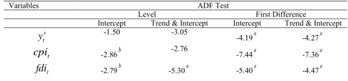
Augmented Dickey-Fuller (1979) and Phillips-Perron (1988) test were applied to check the stationarity of variables. Table 1 includes results of ADF test. According to table 1, inflation
(
cpi
t)
and trade openness (to
t ) are intercept stationary in level. Foreign direct investment(
fdi
t)
on the other hand is stationary in both specifications in level. All other variables are stationary at first difference.Table 1. ADF Unit Root Test
Variables ADF Test
Level First Difference
Intercept Trend & Intercept Intercept Trend & Intercept
s t
y
-1.50 -3.05 -4.19a -4.27a tcpi
-2.86b -2.76 -7.44a -7.36a tfdi
-2.79b -5.30a -5.40a -4.47at
k
-1.47 -2.39 -5.92a -5.83a tgne
-1.80 -1.92 -6.78a -6.72a trem
-1.44 -1.58 -5.77a -5.71a tfd
-0.86 -1.25 -5.29a -5.57a tto
-3.01b -2.97 -7.45a -7.55a 10 % critical values -2.60 -3.19 -2.61 -3.20 1% critical values -3.61 -4.21 -3.62 -4.22Note:
y
ts,cpi
t ,fdi
t,k
t,gne
t,rem
t ,fd
t,to
t Services, etc., value added (% of GDP),Inflation, consumer prices (annual %), external debt as percentage of gross national income, net foreign direct investment, gross fixed capital formation, gross national expenditures, personal remittances received, domestic credit to private sector, money and quasi money ,real exchange rate,
Trade (% of GDP), total population (popt), Permanent cropland (% of land area), respectively.
Superscripts
a
and b show the significance of the estimated parameter at one and ten percentsignificance level respectively.
4.2. Rolling regression
Rolling regressionparameter estimates were obtained by employing OLS within the rolling regression framework for the period 1976–2014. K7 was
set to 12 years. The first observation then dropped and another one added and re-estimated. This process continues until the last observation is used in the analysis. This is in line with the duration of almost one business cycle8
and is in agreement with the choice of Moosa (1997) and Gilal (2013).9
4.3. Rolling regression: Determinants of services sector growth
Graph 1 indicates that the rolling regression estimates of foreign direct investment (
fdi
t ), remittances (rem
t ), inflation (cpi
t ), gross national expenditures (gne
t), gross fixed capital formation (k
t), domestic credit to private sector (fd
t) and trade openness (to
t) with services sector growth (y
st) asdependent variable show some fluctuation. Justification of the use of Kalman filtering approach is that the variables should show some fluctuations.
-.3 -.2 -.1 .0 .1 .2 .3 .4 88909294969800 02040608101214 CPI -.1 .0 .1 .2 .3 .4 .5 8890929496980002040608 101214 FD -.4 -.2 .0 .2 .4 .6 8890 9294969800020406081012 14 FDI -.3 -.2 -.1 .0 .1 .2 .3 88909294969800 02040608101214 GE -.3 -.2 -.1 .0 .1 .2 .3 .4 8890929496980002040608 101214 K -.3 -.2 -.1 .0 .1 .2 .3 .4 8890 9294969800020406081012 14 REM -.2 -.1 .0 .1 .2 .3 88909294969800 02040608101214 TO
Graph 1. Rolling Regression Estimates: Sample period is from 1975 to 2014. In rolling regression window, twelve observations are used. These graphs show rolling regression estimates on equation (1) for inflation(cpi), domestic credit to private sector (fd), foreign direct investment (fdi), gross national expenditures (gne), gross fixed capital formation (k),
4.4. Results comparison: Determinants of services sector growth
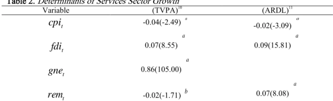
Table 2 shows that inflation ( ) has negative effect on services sector output growth ( ) in case of TVP approach. This result does match with ARDL results. Net foreign direct investment has positive and significant effect on services sector output growth ( ) in both techniques of estimation. Gross national expenditures with positive effect are the relevant significant determinants of services sector output growth ( ) at five percent significance level in case of TVP approach while relationship was insignificant in case of ARDL estimation. Impact of remittances received ( ) on services sector growth ( ) is negative in case of time varying parametric approach. This result is different from ARDL results where relationship was positive and significant at five percent level of significance. The difference of signs is may be due to the impact of structural changes in time varying parametric approach.
Table 2. Determinants of Services Sector Growth
Variable (TVPA)10 (ARDL)11 -0.04(-2.49) -0.02(-3.09) 0.07(8.55) 0.09(15.81) 0.86(105.00) -0.02(-1.71) 0.07(8.08)
Note: and show the significance of estimated parameters at five and ten percent significance
level respectively. Calculated t statistics are given in parentheses.
4.5. State space one step ahead graph (TVPA)
Graph 2 shows one step ahead state vectors that have significant effect on services sector output growth. These state vectors are SV1 (represents inflation), SV2 (represents foreign direct investment) and SV3 (represents gross national expenditure). Graph 2 shows ± two root mean square error one step ahead estimates, after recursive estimation of inflation ( ), foreign direct investment (
) and gross national expenditure ( ) with services sector growth ( ) as dependent variable. It is clear that initially, the estimated parameters show more fluctuation with increased root mean square errors. This is due to a small number of observations that are used for estimating additional parameter of interest. Once the information that is used for predicting t+1 observation increases, the estimated parameters stabilize and their corresponding root mean square errors are reduced. It is further clear from the graph 2 that estimated parameters are stable as they are found to be within the range of ±2 root mean square error.
t cpi t s y t s y t s y t rem yst t cpi a a t fdi a a t gne a t rem b a
a
b t cpi t fdi gnet t s yGraph 2. One step ahead state prediction: SV1, SV2 and SV3 represent inflation (
cpi
t),foreign direct investment (
fdi
t) and gross national expenditure (gne
t)4.6. Stability tests ARDL
Stability of short run and long run model is tested using cumulative sum of recursive residuals (CUSUM) and cumulative sum of recursive residuals square (CUSUMQ). The tests find serious parameter instability if the cumulative sum goes outside the lower and upper critical lines. As it can be seen from graphs 3 and 4, CUMSUM and CUSUMSQ do not cross their critical limits. Hence we conclude that both long run and short run estimates of the model are stable and there is no any structural break.
Graph 3. Testing parameter stability using CUSUM -.3 -.2 -.1 .0 .1 .2 .3 1980 1985 1990 1995 2000 2005 2010 SV1 ± 2 RMSE
One-step-ahead SV1 State Predic tion
-.12 -.08 -.04 .00 .04 .08 .12 .16 1980 1985 1990 1995 2000 2005 2010 SV2 ± 2 RMSE
One-step-ahead SV2 State Predic tion
.70 .75 .80 .85 .90 .95 1980 1985 1990 1995 2000 2005 2010 SV3 ± 2 RMSE
One-step-ahead SV3 State Predic tion
-10.0 -7.5 -5.0 -2.5 0.0 2.5 5.0 7.5 10.0 04 05 06 07 08 09 10 11 12 13 14 CUSUM 5% Significance
Graph 4. Testing parameter stability using CUSUMQ
5. Conclusion
In this study, we examined the determinants services sector growth in Pakistan using time varying parametric estimation technique (Kalman Filter) and auto regression distributed lag(ARDL) bound testing with general to specific approach. Annual data from 1976 to 2014 was used. Choice of sample was based on structural break that resulted country’s disintegration in two wings in 1971. Furthermore, data on most of the variables used in the analysis is available after 1975-76. Rolling regression estimates of explanatory variables justify the use of Kalman filtering approach. Results show that inflation has negative effect on services sector output growth in case of TVP approach. This result does match with ARDL results. Net foreign direct investment has positive and significant effect on services sector output growth in both techniques of estimation. Gross national expenditures with positive effect are the relevant significant determinants of services sector output growth at five percent significance level in case of TVP approach while relationship was insignificant in case of ARDL estimation. Impact of remittances received on services sector growth is negative in case of time varying parametric approach. This result is different from ARDL results where relationship is positive and significant at five percent level of significance. All the one step ahead state vectors confirmed the stability of models in case of time varying parametric approach. Cumulative sum of recursive residuals (CUSUM) and cumulative sum of recursive residuals square (CUSUMQ) also confirmed the stability of results of auto regression distributed lag. Based on these empirical findings, we conclude that government should focus on service sector growth augmenting factors while formulating any policy relevant to the concerned sector.
-0.4 0.0 0.4 0.8 1.2 1.6 04 05 06 07 08 09 10 11 12 13 14
Notes
1
K is used for window size in years i.e. number of observations in rolling regression
2
Belgium, Germany, Greece, Spain, France, Italy, Luxembourg, Netherlands, Austria, Portugal, Finland, Denmark, Sweden and United Kingdom.
3
Generalized least squares is a technique for estimating the unknown parameters in a linear regression model. This technique can be used to perform linear regression when there is a certain degree of correlation between the residuals in a regression model.
4
Through this methodology one can find out the long run relationship in between different time series variables.
5
The detailed discussion of results from both estimation techniques with general to specific approach is not shown here, however, it is available on request.
6
Calculation of F statics, lower and upper bound critical values, and estimation of short run analysis is not shown here, however are available on request.
7
K is used for window size in years i.e. number of observations in rolling regression.
8
The cycles are of the types :1- the Kitchin inventory cycle having duration of 3 to 5 years , 2- the Juglar fixed investment cycle of duration: 7 to 11 years , 4- the Kuznets infrastructural investment cycle having duration of 5 to 25 years and 5- the Kondratieff wave or long technological cycle with duration of 45 to 60 years (Thamae et. al., 2015).
9
Moosa (1997) used 14 observations and Gilal (2013) used 13 observations.
10
These results are taken after employing time varying parametric estimation (TVP) with general to specific approach.
11
Results are taken by employing autoregressive distributive lag (ARDL) bound testing estimation technique with general to specific approach.
References
Agostino, A.D., Serafini, R. & Warmedinger, M.W. (2006). Sectoral explanations of employment in
Europe the role of services. European Central Bank, Working Paper Series, No.625.
Asteriou, D. & Hall, S.G. (2007). Applied Econometrics - A Modern Approach, Basingstoke:
Palgrave Macmillan.
Dickey, D.A., & Fuller, W.A., (1981). Likelihood ratio statistics for autoregressive time series with a
unit root. Econometrica, 49(4), 1057-1072. doi. 10.2307/1912517
Engle, R.F., & Granger, C.W. (1987). Co-integration and error correction: Representation, estimation,
and testing. Econometrica, 55(2), 251-276. doi. 10.2307/1913236
Gilal, A.M., & Chandio, R. (2013). Exchange market pressure and intervention index for Pakistan:
Evidence from a time-varying parameter approach, GSTFJournal on Business Review, 2(4),
18-24. doi. 10.5176/2010-4804_2.4.246
Greiner, A. (2005). Models of economic growth and mathematical models in economics,
Encyclopedia of Life Support Systems (EOLSS), Vol. II.
Gordon, J., & Gupta, P. (2003) Understanding India's services revolution, IMF-NCAER Conference,
A tale of two giants: India’s and China’s experience with reform. pp.1-34.
Hussain, I. (2012). Economic Reforms in Pakistan: One Step Forward, Two Steps Backwards, A
lecture at PIDE.
Hyndman, R., & Snyder, R. (2001). Kalman Filter. [Retrieved from].
Inglesi-Lotz, R. (2011). The evolution of price elasticity of electricity demand in South Africa: A
Kalman Filter application. Energy Policy, 39(6), 3690-3696. doi. 10.1016/j.enpol.2011.03.078
Jain, D., Nair, K.S., & Jain, V. (2015). Factors affecting GDP (Manufacturing, Services, Industry):
An Indian perspective, Annual Research Journal of Symbiosis Centre for Management Studies
Pune, 3, 38-56.
Johansen, S., & Juselius, K. (1990). Maximum likelihood estimation and inference on
cointegration-with applications to the demand for money, Oxford Bulletin of Economics and Statistics, 52(2),
169-210. doi. 10.1111/j.1468-0084.1990.mp52002003.x
Kim, K.H., Zhou, Z., & Wub, W.B. (2010). Non-stationary structural model with time-varying
demand elasticities, Journal of Statistical Planning and Inference, 140(12), 3809-3819. doi.
10.1016/j.jspi.2010.04.045
Lucas, R.E. (1988). On the mechanics of economic development. Journal of Monetary Economics,
22(1), 3-42. doi. 10.1016/0304-3932(88)90168-7
Lutkepohl, H. (2005). New Introduction to Multiple Time Series Analysis. First Edition,
Springer-Verlag Berlin Heidelberg, Germany.
Moosa, I.A. (1997). A cross-country comparison of Okun’s coefficient, Journal of Comparative
Economics, 24(3), 335-356. doi. 10.1006/jcec.1997.1433
Morisson, G.W. & Pike, D.H. (1977). Kalman Filter applied to statistical forecasting, Journal of
Management Sciences, 23(7), 768-774. doi. 10.1287/mnsc.23.7.768
Nkoro, E., & Uko, K.A. (2016). Autoregressive distributed lag (ARDL) cointegration technique:
application and interpretation, Journal of Statistical and Econometric Methods, 5(4), 63-91.
Oyakhilomen, O., & Zibah, R.G. (2014). Agricultural production and economic growth in Nigeria:
implications for rural poverty alleviation. Quarterly Journal of International Agriculture, 53(4),
Pesaran, M.H., Shin, Y., & Smith, R.J. (2001). Bounds testing approaches to the analysis of level
relationship, Journal of Applied Econometrics, 16, 289-326. doi. 10.1002/jae.616
Phillips, P.C.B. & Perron, P. (1988). Testing for unit roots in time series regression, Biometrika,
75(2), 335-346. doi. 10.1093/biomet/75.2.335
Singh, M., & Kaur, K. (2014). India’s services sector and its determinants: An empirical
investigation, Journal of Economics and Development Studies, 2(2), 385-406.
Slade, M.E. (1989). Modeling stochastic and cyclical components of technical change: An application
of the Kalman Filter, Journal of Econometrics, 41(3), 363-383. doi.
10.1016/0304-4076(89)90067-5
Stockman, A. (1981). Anticipated inflation and the capital stock in a cash in-advance economy.
Journal of Monetary Economics, 8(3), 387-393. doi. 10.1016/0304-3932(81)90018-0
Taban, S. (2010). An examinations of governmental spending economic growth nexus for Turkey
using the bound test approach, International Research Journal of Finance and Economics, 48,
184-193.
Thamae, R.I., Thamae, L.Z., & Thamae, T.M. (2015). Dynamics of electricity demand in Lesotho: A
Kalman Filter approach. Studies in Business and Economics, 10(1), 1-10. doi.
10.1515/sbe-2015-0012
Tsadkan, A. (2013). The nexus between public spending and economic growth in Ethiopia: Empirical
investigation. Unpublished Master Thesis, Addis Ababa University.
Viren, M. (2001). The Okun curve is non-linear, Economics Letters, 70(2), 253-57. doi.
10.1016/S0165-1765(00)00370-0
Wu, Y. (2007) Service sector growth in China and India: A comparison. China: An International
Journal, 5(1), 1-20. doi. 10.1142/S021974720700009X
Copyrights
Copyright for this article is retained by the author(s), with first publication rights granted to the journal. This is an open-access article distributed under the terms and conditions of the Creative Commons Attribution license (http://creativecommons.org/licenses/by-nc/4.0).