Abstract. The crowd-sourced Naturewatch GBIF dataset is used to obtain a species classification dataset containing approximately 1.2 mil-lion photos of nearly 20 thousand different species of biological organ-isms observed in their natural habitat. We present a general hierarchical species identification system based on deep convolutional neural networks trained on the NatureWatch dataset. The dataset contains images taken under a wide variety of conditions and is heavily imbalanced, with most species associated with only few images. We apply multi-view classifica-tion as a way to lend more influence to high frequency details, hierarchi-cal fine-tuning to help with class imbalance and provide regularisation, and automatic specificity control for optimising classification depth. Our system achieves 55.8% accuracy when identifying individual species and around 90% accuracy at an average taxonomy depth of 5.1—equivalent to the taxonomic rank of ”family”—when applying automatic specificity control.
Keywords: species identification, convolutional neural networks
1
Introduction
Can we use a commodity camera to take a snapshot of an animal or a plant in the wild and identify its species automatically using convolutional neural networks? This is the question we investigate in this paper, based on a large crowd-sourced image dataset3provided by iNaturalist.org. The data, annotated by experts and deemed research grade, comprises approximately 1.2 million photographs of more than 20 thousand species observed in their natural habitat. It contains images taken by ordinary people under a wide variety of uncontrolled conditions and is heavily imbalanced. On the other hand, the data poses a hierarchical classifica-tion problem, making it possible to abstain from a species-level classificaclassifica-tion if the classification model is insufficiently confident, returning a classification at a higher level of the taxonomy instead.
We use a state-of-the-art pre-trained convolutional neural network, the In-ceptionResnetV2 [10] network trained on the Imagenet [8] data, and fine-tuned it
3
on the Naturewatch data. We introduce two novel techniques—multi-view clas-sification, and hierarchical fine-tuning—along with automatic specificity control for optimising classification depth. Multi-view classification enables the network to retain high frequency details while also increasing representational power, and can be generalised to problems requiring multiple correlated views of an object, while hierarchical fine-tuning helps with class imbalance and provides regularisation.
Our system achieves 55.8% accuracy when identifying species and around 90% accuracy at an average taxonomy depth of 5.1—equivalent to the taxonomic rank of ’family’—when applying automatic specificity control.
Species identification using machine learning is not a new idea and has been attempted before, but in a much more constraint setting on a much smaller scale. We review related work in the next section before presenting our deep-learning-based system in Section 3. Section 4 describes how we prepared the data and Section 5 presents our results. Section 6 concludes the paper.
2
Related work
Classification of moths is the subject of [6], based on a dataset containing 774 images across 35 classes. Images are mostly dorsal views of moths on a uni-formly coloured background. Prior to classification with a support vector ma-chine, global image statistics, colour histograms, local patch intensity statistics and other features are extracted from each image. The system achieves an accu-racy of 85% in 10-fold cross validation.
Colour histogram features are also used for species classification in [7], but in the context of constructing hierarchically structured ensembles of neural net-works trained using evolutionary optimisers. The classification hierarchy is tra-versed from the topmost level (genus) down to the species level to produce labels. If insufficient information is provided to the classifier, traversal is stopped and a less specific label produced. This is similar to the hierarchical approach we present in this paper. The classifier is evaluated on images of orchids.
A different set of features is used in [13], which presents experiments on a dataset of 120 images across seven species. The images are processed by an edge detector and have their contours digitised with the elliptic Fourier transform. A support vector machine classifier is trained on the elliptic Fourier coefficients, yielding a final per-species accuracy ranging from 90% to 98% .
Deep convolutional networks have also been considered for species classifica-tion. In [5], a fine-tuned deep convolutional neural network classifier for plant leaves is presented, using a dataset consisting of 2816 images across 44 classes of plant leaves. The system achieves an accuracy of 99.5%, demonstrating the efficacy of convolutional neural networks.
Deep neural networks are also used in [2], which applies a technique similar to HD-CNN [12] over a base network of fine-tuned VGGNets. With 200k im-ages spread across 277 classes, this method attains an accuracy of 44.6%. As in our work, the images are commodity images taken in various conditions and
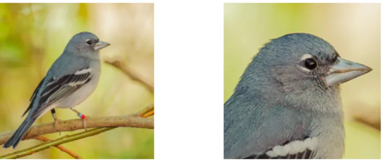
Fig. 1: A visualisation of the two views the network receives
backgrounds. Along with the relatively large number of classes this is a likely explanation for the relatively low accuracy.
3
Hierarchical species classification with deep learning
We use a modified version of the InceptionResnetV2 network trained on the Imagenet data as the starting point for our experiments. The modified version of the network has a different architecture than the one described in [10], and makes use of auxiliary classifiers as in [11]. In the following, we describe how we apply multi-view classification, hierarchical knowledge transfer, and automatic specificity control to yield our final system.
3.1 Multi-view classification
Our multi-view network architecture is inspired by three related works. In [3], two different scales of video frames are used for video classification—one neural network is trained on the entire image region, and another on only the central region. The outputs of the two networks are merged at the ”bottleneck” layer and classification is performed from there. In [9], a network composed of multiple views of an object is trained and combined using pooling, with the results being passed to another convolutional neural network for final classification. All views of the object are passed through the same initial network which acts as a feature extractor. Finally, in TreeNets, as presented in [4], the authors demonstrate that branching of networks after a few layers and ensembling the results, instead of branching at input—as for normal ensembles—results in useful sharing of common early-level convolutional filters general to most images, and leads to increased accuracy.
Our multi-view classification technique uses two sections of the input image, both at the same resolution but at different magnification scales, to perform training and classification.This is important for species identification as both the high frequency details and the overall shape of the image have a significant impact on what the species is. The first five convolution layers of our architec-ture act as a shared feaarchitec-ture extractor for both views. Parameters are shared
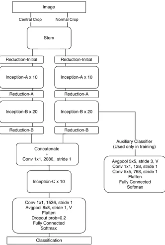
up to and including the stem block of the architecture, after which the network splits into two, each with its own set of parameters. To allow features from the different input images to correlate with each other, we concatenate the output of the two branches, doubling the depth, and perform a 1x1 convolution with output depth equal to that before concatenation. We then use the rest of the InceptionResnetV2 network’s pipeline as normal. See Figure 2 for the overall network architecture.
One issue with our multi-view technique is that during training time, the region of interest is not known and thus we compromise and take the central region. However, if the object of interest is not within the central region, then this may lead to an unexpected combination of features leading to a possibly misinformed classification. One way of overcoming this obstacle would be to use a training set with bounding boxes on objects of interest. Then, during classification, the user could be asked to specify a bounding box for the region of interest.
Network specific adjustments Google’s Inception series of networks use an auxiliary classifier [11] as an additional source to optimise for. We keep the auxiliary classifier only on the whole-view branch. Another adjustment we make is that the crop-view branch is not initialised from a pretrained network but randomly, to encourage diversity between the two branch networks. As the layers before and after this branch both have pretrained weights, this branch should quickly adapt [14] to the training data.
3.2 Hierarchical knowledge transfer
Overfitting is an acute problem when dealing with very small classes containing few observations. Given the hierarchical nature of our dataset, we combat this problem by translating labels to those of their superclasses, effectively reducing the number of classes and increasing the number of samples per class.4This can be applied recursively up the hierarchy until a desired number of samples-per-class is achieved. We then first train against this reduced-complexity problem, progressively increasing the difficulty of the dataset by translating labels down the hierarchy and copying final-layer weights to the corresponding subclasses. This is done recursively until the original problem is recovered.
Formally, letkd be the number of different classes at depthd,X be the set of input examples,d0∈ {0, . . . , dmax−1} be the starting depth, andwd be the weights of the (currently) final layer of the network, for classifying at depth d. Moreover, let f : X×W → {1, . . . , kd} be the model classifying an example using weightswandtd :{1, . . . , kd} → {1, . . . , kd−1}be the translation function at depthdthat maps a label to its parent label.
We optimisef using wd0 until convergence, then create new weightswd+1, where weights for each class i are set according to wd(i+1) = w(td(i))
d . Finally, 4
Fig. 2: Multi-view network architecture
to obtain diversity in the weight vectors, we mix in randomisation for wd+1 as explained below. We continue this process, incrementingduntil d=dmax.
The aim of this process—through the combined effect of smoother error sur-faces due to the simpler problems being initially tackled, and superclass-based weight initialisation—is to achieve a strong regularising effect and enhance clas-sification accuracy for under-represented classes. This technique also aids conver-gence speed as superclasses usually have more distinguishing features between them, helping the network quickly locate the features that actually matter.
Weight vector randomization Here we will derive the expression for mixing weights. We will be using uniform distributions for adding randomness as it was the initialisation method used in the base network architecture InceptionRes-netV2. We want to mix the two weights using a user-determined scalar factor
vari-ance. LetX,Y be independent random variables with equal variances such that
V ar[X] =V ar[Y]. For any scaled distribution,
V ar[kX] =k2V ar[X]
thus to recover the original variance we need to scaleX andY by√aand√1−a:
V ar[√aX+√1−aY] =aV ar[X] + (1−a)V ar[Y] =V ar[X] =V ar[Y]
Therefore, to maintain the original variance, we mix weights according to: w=√aw0+√1−awrandom
3.3 Automatic specificity adjustment
Given the nature of our data it is clear that we will not achieve high accuracy across the full set of species. We can try to avoid presenting misleading infor-mation to the user of our system by classifying at higher levels of the hierarchy when necessary. The method presented in [1] classifies the input along a given hierarchy such that maximum information gain is achieved, while maintaining a targeted accuracy. It is based on the observation that classifying at the root node of the hierarchy would result in perfect accuracy, but with zero information gain, while always classifying at a leaf node would maximise information gain, but yield potentially low accuracy. A threshold dictates the cut-off point that is used to determine which level of the hierarchy an input is classified at, such that information gain is maximised while satisfying an accuracy target. The optimal threshold is found using binary search on accuracy values obtained through eval-uating the test set against the current threshold. In operation, real data is, of course, different from that in the test set, and thus this method cannot guarantee accuracy given unseen examples.
For our work, we use the absolute depth as the metric instead of information gain, as information gain has little bearing in terms of species classification. We classify at the deepest node that provides an estimated class probability greater or equal to the user-provided confidence threshold. Additionally, we allow one to specify a series of prior nodes to begin search from, instead of always using the hierarchy root, such that users with additional information can improve their classification accuracy and granularity.
To classify at a level higher than leaf level, some method must be employed to produce class probability estimates for those higher level nodes. One method is to climb up the hierarchy from the most likely leaf class but this does not yield a probability; another is to use separate classifiers for each branching point, which is unsuitable for large and computationally complex networks such as InceptionResnetV2. Yet another one is to approximate class probabilities for higher-level nodes as the sums of all probabilities of successor nodes. The last method is what we use in this paper.
The goal is the to find argmax
n
Depth(n) +N odeP robability(n) subject to N odeP robability(n)< t
An optimal way to find this node is to traverse the tree in a depth-first manner such that depths and probabilities are obtained whenever a node’s children have been traversed.
As the test set is not an exact representation of real data, there is little need for having a mathematically guaranteed accuracy in practical scenarios. A probabilistic approximation may serve the purpose whilst taking significantly less time to optimise. Under this assumption, we build on the prior work in [1] in that instead of using full binary search for the best threshold, we use hill-climbing to optimise the threshold parameter with regards to a target accuracy while running the evaluation. With a learning factor that reduces as optimisation proceeds, we can converge to a threshold that nearly maximises specificity while hitting the target accuracy. Hill climbing is effective in this case as an increase in threshold and will always lead to an increase in accuracy.
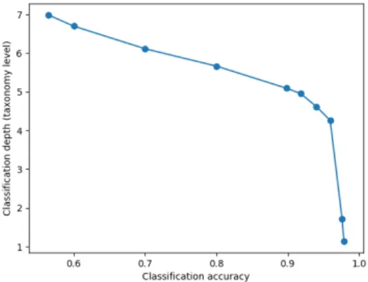
One can see in Figure 3 that there is always a trade-off between target accu-racy and classification depth. As we approach a target accuaccu-racy of 1, classification depth decreases sharply, as even root level nodes fail to classify to the specified accuracy. A graph like this can be useful in inferring a target accuracy that still provides results at a meaningful depth.
4
Data preparation
Our image set exhibits a significant number of challenges. The distance from camera, lighting conditions, background, and image quality are very variable. The same species could look drastically different in two given images. Further-more, species may be at any stage in their lifecycle—for example images labelled as a monarch butterfly may represent this species in egg or butterfly form. The image may not contain the labelled species at all—foot prints, faecal matter, and other identifiable aspects may be present in the image set, which leads to the next point: the expert labelling may be based on more than the image itself, taking into account location, time and the submitted text brief to produce a la-belling. The images may also contain more than one species. These issues make it extremely challenging for the classifier to build a robust model. We should also note that our species hierarchy is a taxonomic hierarchy and not necessarily based on visual differences. Behaviour, habitat, and genome sequence are often key differentiators in the taxonomy but cannot necessarily be captured in images. Given a hierarchy corresponding to the visual similarity between the classes, the accuracy of classification would likely improve.
The full dataset consisted of images separated into over 100,000 different species. These images are mostly in JPEG format with resolutions ranging from 0.3 to over eight megapixels. Non-JPEG images were not downloaded for our experiments. Also, during the downloading process, some images could not be retrieved, and some of the species had an unusual taxonomy and were discarded. Many species had fewer than five images under their name, making it unsuitable for training a deep learning type model. Such images were also discarded. Finally, the dataset of usable images consisted of 1,214,141 images across 19,027 classes. The dataset was randomly separated into 2 sets, training and validation, in a 80-20 split. The training set was used for training, while the validation set was used to test and measure classification accuracy. In total, 16,583 species were present in the validation set, instead of the full 19,027 in the training set. As a standard practice to improve accuracy, these selected images underwent random augmentation when training the network, where each image entered into the network was cropped, horizontal-flipped with a random chance, and had its brightness adjusted by ±12.5%, contrast adjusted by ±50%, hue adjusted by
±20% and saturation adjusted by±50%. Vertical flipping and rotation was not used for augmentation as almost all plant or animals are captured at a certain angle. The augmentation was performed in a stream-wise manner as images were loaded in for training.
– Adam optimiser withβ1= 0.9,β2= 0.999 and= 1
Parameter tuning was not performed, to enable a more controlled comparison between the different networks used. Further optimising hyperparameters may lead to an increase in accuracy.
For automatic specificity adjustment, we targeted an accuracy of 90%. We split the validation set into two even parts, with one part not being used to affect the confidence threshold. The average classification depth and accuracy was based solely off the unseen set of 100,000 images. We reused this configuration for all three of our experiments concerning automatic specificity adjustment.
Our first experiment with the large dataset was with a pretrained and un-modified InceptionResnetV2 network. For this experiment, a batch size of 32 was used. We trained for a total of six epochs, using a learning rate of 0.01 for the first three epochs, followed by 0.001 for the next two, and 0.0001 for the final one. A final accuracy of 46.6% was attained. Using automatic specificity adjustment, we achieved an accuracy of 90.0% at an average taxonomy depth of 4.78.
Our second experiment used the modified multi-view InceptionResnetV2 net-work. For this experiment, a batch size of 16 was used, due to the increased model size, forcing us to reduce batch size to free up enough memory. We trained for a total of four epochs, using a learning rate of 0.1 for the first two epochs, followed by 0.01 for the next one-and-a-half, 0.001 for the next half, and 0.0001 for the final half epoch. A final accuracy of 54.8% was attained, an increase of 9.2% above the state-of-the-art InceptionResnetV2 network. Using automatic speci-ficity adjustment, we achieved an accuracy of 90.0% at an average taxonomy depth of 4.96, which is a 5.6% increase in depth. When testing on the training set, an accuracy of 68.2% was attained—a significant increase over that on the validation set, which shows signs that the network is overfitting.
Our third experiment used the multi-view InceptionResnetV2 network along with the hierarchical knowledge transfer technique. A batch size of 16 was again used. Training was done in two stages—first we trained at the genus level (tax-onomy level 6) over one-and-a-half epochs using a learning rate of 0.1. Then we translated and trained at the species level (taxonomy level 7) for three more epochs, using a learning rate of 0.1 for the first epoch, 0.01 for the next one, 0.001 for the next half, and 0.001 for the final half. A final accuracy of 55.8% was attained, an increase of 1.0% above what we achieved with the multi-view Incep-tionResnetV2 network. Using automatic specificity adjustment, we achieved an
accuracy of 90.0% at an average taxonomy depth of 5.09, which is a further 3.3% increase above the depth in the previous experiment. Interestingly, when tested on the training set, an accuracy of 57.8% was attained. Compared to using the multi-view approach alone, we see that applying hierarchical knowledge transfer reduces the amount of overfitting significantly.
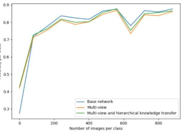
Fig. 4: The differences in accuracy for classes of different sizes, for the three experiments.
In Figure 4 we can see that multi-view networks provided a large improve-ment in accuracy for small classes, at the cost of reduced accuracy for larger classes. We speculate that this is due to the improved model being more able to distinguish the small difficult classes, thus no longer sacrificing their accuracy for those of the larger, easier classes. Surprisingly, hierarchical knowledge transfer provided gains across all class sizes. This goes against the initial hypothesis in Section 3.2 and means that, at least in this dataset, not only under-represented classes but all classes, benefit from the pretraining and initialisation from pa-rameters of superclasses. It is interesting to note from Table 1 that although hierarchical knowledge transfer gains only 1% improvement in raw accuracy, it delivers 3.3% increased classification depth at the same target accuracy when automatic specificity adjustment is applied, while multi-view learning alone de-livered a 9.2% increase in raw accuracy but only a 5.6% increase in classification depth.
6
Conclusions
We investigated the viability of large-scale species identification from commodity images using state-of-the-art image recognition based on a convolutional neural
network. The experimental results are highly encouraging, with 55.8% classifica-tion accuracy when discriminating between the almost 20,000 individual species in the dataset and 90.0% accuracy at an average taxonomy depth of 5.1 when applying automatic specificity control.
There is potential for the developed system to be used in a diverse range of applications, for example, identifying tree species in autonomous UAV surveys, or classifying harmful pests in one’s backyard. However, for more critical ap-plications, the granularity or accuracy may not yet be sufficient. The primary reason for this is that many species in the dataset are represented by very few images.
Two of the methods considered in this paper, hierarchical knowledge transfer and multi-view classification, may warrant investigation in other classification settings as well. Moreover, it would be useful to consider the effect of tuning the parameters for hierarchical knowledge transfer and experimenting with ar-chitecture variations for multi-view classification. The latter technique could be generalised to any classification task that requires different views of an object. For each additional view, we can add another column after the initial split point in the network and merge at the concatenation point. These multiple views may stem from different images or from sub-regions of the same image as in this pa-per. Depending on the similarity of features in these views, the network should be tuned such that an appropriate amount of parameters is shared between views.
Acknowledgements
We would like to acknowledge financial support from the MBIE Endeavour re-search grant ”Biosecure-ID”. We would like to thank Dr. Michael Cree for many useful discussions and Dr. Jerry Cooper and Dr. Aaron Wilton as the experts behind NatureWatch for their contribution.
References
1. Deng, J., Krause, J., Berg, A.C., Fei-Fei, L.: Hedging your bets: Optimizing accuracy-specificity trade-offs in large scale visual recognition. In: Proceedings of the 2012 IEEE Conference on Computer Vision and Pattern Recognition. pp. 3450– 3457. IEEE (2012)
2. Glick, J., Miller, K.: Insect classification with heirarchical deep convolutional neural networks (2016), http://cs231n.stanford.edu/reports/2016/pdfs/283 Report.pdf, Final report for Convolutional Neural Networks for Visual Recognition (CS231N), Stanford University
3. Karpathy, A., Toderici, G., Shetty, S., Leung, T., Sukthankar, R., Fei-Fei, L.: Large-scale video classification with convolutional neural networks. In: Proceedings of the 2014 IEEE Conference on Computer Vision and Pattern Recognition. pp. 1725– 1732. IEEE (2014)
4. Lee, S., Purushwalkam, S., Cogswell, M., Crandall, D., Batra, D.: Whym heads are better than one: Training a diverse ensemble of deep networks. arXiv preprint arXiv:1511.06314 (2015)
5. Lee, S.H., Chan, C.S., Wilkin, P., Remagnino, P.: Deep-plant: Plant identification with convolutional neural networks. In: Proceedings of the 2015 IEEE International Conference on Image Processing. pp. 452–456. IEEE (2015)
6. Mayo, M., Watson, A.T.: Automatic species identification of live moths. Know.-Based Syst. 20(2), 195–202 (Mar 2007)
7. Pereira, S., Gravendeel, B., Wijntjes, P., Vos, R.: Orchid: a generalized frame-work for taxonomic classification of images using evolved artificial neural netframe-works. bioRxiv preprint 070904 (2016)
8. Russakovsky, O., Deng, J., Su, H., Krause, J., Satheesh, S., Ma, S., Huang, Z., Karpathy, A., Khosla, A., Bernstein, M., Berg, A.C., Fei-Fei, L.: ImageNet Large Scale Visual Recognition Challenge. International Journal of Computer Vision 115(3), 211–252 (2015)
9. Su, H., Maji, S., Kalogerakis, E., Learned-Miller, E.: Multi-view convolutional neural networks for 3d shape recognition. In: Proceedings of the 2015 IEEE Inter-national Conference on Computer Vision. pp. 945–953. IEEE (2015)
10. Szegedy, C., Ioffe, S., Vanhoucke, V., Alemi, A.A.: Inception-v4, inception-resnet and the impact of residual connections on learning. Proceedings of the 3st AAAI Conference on Artificial Intelligence (2017)
11. Szegedy, C., Vanhoucke, V., Ioffe, S., Shlens, J., Wojna, Z.: Rethinking the incep-tion architecture for computer vision. In: Proceedings of the 2016 IEEE Conference on Computer Vision and Pattern Recognition. pp. 2818–2826. IEEE (2016) 12. Yan, Z., Zhang, H., Piramuthu, R., Jagadeesh, V., DeCoste, D., Di, W., Yu, Y.:
HD-CNN: Hierarchical deep convolutional neural network for large scale visual recognition. In: Proceedings of the 2015 IEEE Conference on Computer Vision and Pattern Recognition. pp. 2740–2748. IEEE (2015)
13. Yang, H.P., Ma, C.S., Wen, H., Zhan, Q.B., Wang, X.L.: A tool for developing an automatic insect identification system based on wing outlines. Scientific Reports 5(12786) (2015)
14. Yosinski, J., Clune, J., Bengio, Y., Lipson, H.: How transferable are features in deep neural networks? In: Advances in Neural Information Processing Systems 27. pp. 3320–3328. Curran Associates, Inc. (2014)