Institutional Knowledge at Singapore Management University
Research Collection School Of Information Systems
School of Information Systems
2014
Online Multiple Kernel Similarity Learning for
Visual Search
Hao Xia
Chu Hong HOI
Singapore Management University, [email protected]
Rong Jin
Peilin Zhao
DOI:
https://doi.org/10.1109/TPAMI.2013.149
Follow this and additional works at:
https://ink.library.smu.edu.sg/sis_research
Part of the
Computer Sciences Commons
This Journal Article is brought to you for free and open access by the School of Information Systems at Institutional Knowledge at Singapore Management University. It has been accepted for inclusion in Research Collection School Of Information Systems by an authorized administrator of Institutional Knowledge at Singapore Management University. For more information, please [email protected].
Citation
Xia, Hao; HOI, Chu Hong; Jin, Rong; and Zhao, Peilin. Online Multiple Kernel Similarity Learning for Visual Search. (2014).IEEE Transactions on Pattern Analysis Machine Intelligence (TPAMI). 36, (3), 536-549. Research Collection School Of Information Systems. Available at:https://ink.library.smu.edu.sg/sis_research/2284
Online Multiple Kernel Similarity Learning for
Visual Search
Hao Xia, Steven C.H. Hoi, Rong Jin, Peilin Zhao
Abstract—Recent years have witnessed a number of studies on distance metric learning to improve visual similarity search in
Content-Based Image Retrieval (CBIR). Despite their successes, most existing methods on distance metric learning are limited in two aspects. First, they usually assume the target proximity function follows the family of Mahalanobis distances, which limits their capacity of measuring similarity of complex patterns in real applications. Second, they often cannot effectively handle the similarity measure of multi-modal data that may originate from multiple resources. To overcome these limitations, this paper investigates an online kernel similarity learning framework for learning kernel-based proximity functions, which goes beyond the conventional linear distance metric learning approaches. Based on the framework, we propose a novel Online Multiple Kernel Similarity (OMKS) learning method, which learns a flexible nonlinear proximity function with multiple kernels to improve visual similarity search in CBIR. We evaluate the proposed technique for CBIR on a variety of image data sets, in which encouraging results show that OMKS outperforms the state-of-the-art techniques significantly.
Index Terms—Similarity search, kernel methods, multiple kernel learning, online learning, content-based image retrieval
✦
1
I
NTRODUCTIONSimilarity search plays a fundamental role in a variety of multimedia retrieval tasks [1], [2], [3], which has been extensively studied in multimedia and computer vi-sion fields, especially for Content-Based Image Retrieval (CBIR) [4], [5], [6]. The crux of visual similarity search is to find some proximity function that can effectively measure distance/similarity between images [7], [8]. In a conventional CBIR system, given images represented in a vector space, the typical choices of such proximity functions are Euclidean distance and its variants, which are often not flexible enough to measure the proximity of images due to the nature of the fixed rigid functions. In recent years, researchers have noticed the limita-tions of conventional rigid proximity funclimita-tions in image similarity search. To address this issue, one group of active research studies are the Distance Metric Learning (DML) algorithms [5], [9], [10], [11], which usually learn to optimize the distance metric of proximity measure to improve image similarity search in CBIR. Despite the success of various DML algorithms to improve similar-ity search of CBIR, most existing DML algorithms are limited in two aspects. First, they typically assume the target proximity function follows the form of general Mahalanobis distances and restricts the DML task in finding an optimal linear distance metric, which may limit its capacity of measuring similarity of complex image patterns in real applications. Second, even though
• H. Xia, S.C.H. Hoi, and P. Zhao are with the School of Computer
Engineering, Nanyang Technological University, Singapore.
R. Jin is with the Department of Computer Science and Engineering, Michigan State University, United States.
Corresponding E-mail: [email protected]
there are few existing works [12], [13] for learning non-linear similarity function with kernel, they usually do not handle the similarity with multiple kernels.
To overcome the limitations of existing work, in this paper, we propose a novel Online Multiple Kernel Sim-ilarity (OMKS) learning scheme, which ranks images by learning pairwise similarity of images that are rep-resented in multiple modalities using multiple kernels. Unlike the conventional DML techniques, the target similarity function learned by OMKS can be any nonlin-ear function in some reproducing kernel Hilbert spaces induced by some predefined kernels. And different from some batch kernel-based DML algorithms, OMKS learns with multiple kernels in an online learning fashion [14]. Thus, OMKS is able to learn a much more flexible and powerful proximity function to improve image similarity search in CBIR.
The OMKS task is however very challenging because it must on one hand learn an optimal kernel-based similar-ity function for each kernel in each modalsimilar-ity, and on the other hand determine an optimal combination of multi-ple kernels in building the final similarity function for similarity search with all modalities. To attack the chal-lenges, we propose a unifying online learning scheme for OMKS, which learns both the optimal similarity function with each individual kernel and the optimal combi-nation of multiple kernels in a coherent and scalable online learning framework. In particular, we apply the online passive aggressive learning technique [15] to learn the kernel-based similarity function for each individual kernel, and the well-known Hedging online learning technique to learn the optimal combination weights of multiple kernels, from a sequence of triplet training data. As a summary, our key contributions include:
kernel-based proximity functions with multiple kernels for visual similarity search. To the best of our knowl-edge, this is the first online learning work in CBIR that learns to rank images based on kernel-based similarity function using multiple kernels.
• We present an online learning algorithm for OMKS,
which learns both the optimal kernel-based simi-larity function with an individual kernel and the optimal combination of multiple kernels.
• We conduct an extensive set of experiments to
eval-uate the performance of the proposed technique for CBIR on several image data sets.
The rest of this paper is organized as follows. Section 2 reviews related work. Section 3 gives some preliminaries of the related techniques. Section 4 introduces the prob-lem definition and presents the proposed online learning algorithm for OMKS, followed by theoretical analysis in Section 5. Section 6 discusses the experimental results, and section 7 sets out the conclusion of this work.
2
R
ELATEDW
ORKThis section reviews related work which can be generally grouped into three major categories as follows.
2.1 Distance Metric Learning
Distance Metric Learning (DML) from side information (e.g., relevance feedback logs [16] or user-generated con-tents of social images [17]) has been actively studied in CBIR for several years. In general, most DML works aim to learn an optimal distance metric in the family of Ma-halanobis distances, which can be viewed as an equiva-lent problem of learning an optimal linear projection of original data into a new space, where Euclidean distance is adopted to measure proximity between objects.
In literature, various DML techniques have been proposed in both machine learning [18], [19], [20] and multimedia [5], [9], [10], [21], [22]. Some well-known techniques include Relevant Component Anal-ysis (RCA) [18], Discriminative Component AnalAnal-ysis (DCA) [5] using the idea of Fisher’s Linear Discriminant Analysis, Large Margin Nearest Neighbor (LMNN) [20], Metric Learning by Collapsing Classes [23], learning globally-consistent local distance functions [24], Reg-ularized Distance Metric Learning [9] and Laplacian Regularized Metric Learning (LRML) [11], and so on.
In general, the DML task is cast as a Semi-Definite Pro-gramming (SDP) problem due to the impose of Positive Semi-Definite (PSD) constraint on the solution, which is computationally intensive, especially when data is of high dimensionality. Some recent work has attempted to resolve the challenge, such as ITML [25] and OA-SIS [26]. ITML uses LogDet divergence which can en-force positive semi-definiteness automatically to bypass the PSD constraint. OASIS drops the PSD constraint and resolves the DML task by an online learning algorithm to maximize the large margin criterion. OASIS is in
general a linear metric learning method. Our technique is partially inspired to overcome the limitations of OASIS by studying kernel-based learning techniques.
2.2 Kernel-based Learning for Image Retrieval
Kernel-based learning techniques are not new for image retrieval. Our technique differs from the existing kernel-based learning techniques proposed for image retrieval in literature. For example, kernel SVM algorithms have been proposed for active learning in CBIR [27], which however address different types of problems as ours.
In literature, several kernel-based distance metric learning algorithms [28], [29] were proposed for learning similarity functions in CBIR. Also, a family of metric learning algorithms including LMNN and NCA have been shown to be able to be kernelized by KPCA trick [12]. Some recent work also reveals the connections between metric and kernel learning in [13], which may naturally provide kernelization for a larger class of met-ric learning methods. Our techniques differ from these approaches in two key aspects. First, they are designed to learn with a single kernel while the proposed algorithm learns with multiple kernels; and second, they usually run in a batch learning approach, which does not scale to large-scale applications. In contrast, we present online learning algorithms for learning a similarity function with multiple kernels.
We also note that our work is very different from exist-ing kernel learnexist-ing studies, such as KernelBoost [30] and nonparametric kernel learning [31], [32], which mainly aim to learn a kernel function/matrix consistent with given constraints. Unlike these studies, the proposed technique learns a kernel-based similarity function, in-stead of a kernel function, from constraints.
Finally, some recent studies also proposed online learning techniques to learn kernel-based similarity func-tion for text-based image search. For example, PAMIR [3] proposed to learn a discriminative model for the image retrieval from text queries using online learning tech-niques. Our study differs from PAMIR because PAMIR is specially designed for text-based queries and thus cannot be directly applied to the CBIR task.
2.3 Multiple Kernel Learning
Our work is also closely related to Multiple Kernel Learning (MKL) studies [33], [34], which aim to find the optimal combination of multiple kernels for learning classifiers towards a given classification task. Exemplar algorithms include the convex optimization [33], the Semi-Infinite Linear Program (SILP) approach [34], and the level method [35]. In addition, several recent stud-ies [36], [37] address multiple kernel learning for multi-class and multi-labeled data, and some other works aim at improving its efficiency and generality [38], [39], [40]. Despite sharing the common goal of finding the op-timal combination of multiple kernels, our technique differs significantly from the existing MKL studies in two
key aspects. First, we aim to learn kernel-based proxim-ity functions for image ranking tasks while conventional MKL studies often address classification tasks. Second, the training data used by conventional MKL studies are in the regular form of single data instances with class label, while the training data in our problem are in the form of triplet instances.
We should note that this work was also inspired by our previous work on Online Multiple Kernel Learning (OMKL) [41], [42]. The OMKL technique was proposed to learn classifiers by finding an optimal combination of multiple kernels for classification tasks, while the goal of this work is to learn the image similarity function from triplets for retrieval tasks in CBIR. In particular, special care is needed in the design of algorithms to handle the triple constraints. Finally, although MKL has successfully been applied to several computer vision applications [43], [44], to the best of our knowledge, this is the first online learning work that learns a similarity function using multiple kernels for CBIR.
3
P
RELIMINARIESTo better motivate our work, we introduce some prelim-inaries of two closely related techniques: (1) online mul-tiple kernel learning, and (2) large scale online learning of image similarity through ranking.
3.1 OMKL
We briefly review the recent work on Online Multiple Kernel Learning (OMKL) [41], [42]. This technique in general aims to address a Multiple Kernel Learning (MKL) problem.
Specifically, given a set of training examples D =
{(xi, yi), i= 1, . . . , n} where yi ∈ {−1,+1}, i= 1, . . . , n,
and a collection ofmkernel functionsK={κi:X ×X →
R, i= 1, . . . , m}, the goal of an MKL task is to identify the optimal combination of the kernel matrices, denoted by θ= (θ1, . . . , θm), which minimizes the margin-based
classification error. This can be formulated as the follow-ing optimization task:
min θ∈∆f∈HminK(θ) 1 2kfk 2 HK(θ)+C n X i=1 l(f(xi), yi) (1) where K(θ)(·,·) = Pmi=1θiκi(·,·), l(f(xi), yi) =
max(0,1−yif(xi)), and∆ is defined by
∆ ={θ∈Rm+|θTem= 1}. (2)
The OMKL technique simplifies the MKL problem by learning the following classification function with multiple kernels: f(x) = m X i=1 θisign(fi(x)) (3)
The OMKL algorithm iteratively updates the predic-tion funcpredic-tion by the perceptron algorithm, i.e.,
ft+1,i(x) =ft,i(x) +zi(t)ytκi(xt, x) (4)
and learns the combination weights by applying the Hedging online learning technique, i.e.,
θi(t+ 1) =θi(t)βzi(t) (5)
whereβ∈(0,1)is a discount weight parameter, which is employed to penalize the kernel classifier that performs incorrect prediction at each learning step, andzi(t)
indi-cates if thei-th kernel classifier makes a mistake on the prediction of the examplext.
3.2 OASIS
Below we briefly introduce another related work of large scale online learning of image similarity through ranking [26]. Specially, the goal of this problem is to learn a similarity function S(pi, pj) that assigns higher
similarity scores to pairs of more relevant images, i.e.,
S(pi, p+i )> S(pi, pi−), ∀pi, p+i , p−i ∈P (6)
such that r(pi, p+i)> r(pi, p−i ) (7)
wherer(·,·)reflects the relevance between two images. Consider a parametric similarity function that has a bi-linear form, SW(pi, pj) = piTW pj where W ∈ Rd×d, the
goal is to find a parametric similarity function S such that all triplets obey the following constraints:
SW(pi, p+i)> SW(pi, p−i ) + 1 (8)
One can define the following hinge loss function for the triplet:
lW(pi, p+i , p−i ) = max{0,1−SW(pi, p+i )+SW(pi, p−i )} (9)
As a result, thebatch optimization problem of this task can be formulated as:
W = arg min W kWk 2 F ro+C X i ℓW(pi, p+i , p−i ) (10)
Theonline optimization problem is formulated as:
Wi= arg min W 1 2kW−Wi−1k 2 F ro+CℓW(pi, p+i , p−i ) (11)
By initializing W0 =I, the online solution of updating W is given as: Wi=Wi−1+τiVi (12) whereτi= min{C, lWi−1(pi,p+i,p−i) kVik2 }andVi=pi(p + i −p−i )T.
4
O
NLINEM
ULTIPLEK
ERNELS
IMILARITYWe first present our framework for online kernel similar-ity learning, and then extend it to online multiple kernel similarity learning.
Training Triplet (pt,pt+,pt-)
Model Updating
OKS Model forκ1
S1(q,p)
OMKS Model f(q,p)=∑iθiSi(q,p)
θ1
OKS Model forκi
Si(q,p)
θi
OKS Model forκm
Sm(q,p) θm .. . Image Database Query Image Computing Similarity Scores
Similarity Scores Ranked List
Training Phase Retrieval Phase
Model Updating
Model Updating
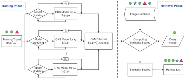
Fig. 1. The system flow of the proposed online multiple kernel similarity learning scheme for visual search.
4.1 Online Kernel Similarity
Our challenge is how to extend the linear similarity function used in OASIS to its kernel version. To this end, for a given kernel κ(·,·) and the corresponding Hilbert spaceH, we introduce a linear operatorL:H 7→ Hthat maps a function f ∈ H to another function L[f] ∈ H. Given the linear operator L, we define the similarity function SL(p, q)as
SL(q, p) =hκ(q,·), L[κ(p,·)]iH (13)
q ∈ X is a query image and p ∈ X is an image in
database to be retrieved. Compared to the similarity function SW(p, q) = p⊤W q, we observe that the linear
operator L plays the same role as matrix W. Let L be
the space that includes all the linear operators inH, i.e.,
L={L:H 7→ H, Lis a linear operator} (14) Following the framework of OASIS, we develop a frame-work of kernel similarity learning based on the linear operator. It searches for the optimal linear operator by minimizing the rank loss, i.e.,
L∗ = arg min L∈LkLk 2 HS+C X i ℓL(pi, p+i , p−i ) (15)
where k · kHS is the Hilbert Schmidt norm
of the linear operator, and ℓL(pi, p+i , p−i ) =
max 0,1−SL(pi, pi+) +SL(pi, p−i )
.
Next, we develop an online learning algorithm for ef-ficiently solving (15) based on the online Passive Aggres-sive (PA) learning [15]. Similar to the OASIS algorithm, in the proposed online learning algorithm, at each trial
t, given tripletpt, p+t, p−t, we solve the following simple
optimization problem Lt= arg min L∈L 1 2kL−Lt−1k 2 HS+CℓL(pt, p+t, p−t) (16)
where we initialize L0 to be an identity operator at the
beginning of online learning. The following proposition
gives the closed-form solution to the above optimization.
Proposition 1: The optimal solution to the optimization problem in (16) can be expressed as:
Lt=Lt−1+τtZt (17)
whereZt∈ Lis a rank one linear operator and is given
byZt[h](·) =κ(pt,·) h(p+t)−h(p−t)
for anyh∈ H. The coefficientτt in (17) is calculated as τt= min ( C, max{0,1−SLt−1(pt, p + t) +SLt−1(pt, p−t)} κ(pt, pt)(κ(p+t, p+t)−2κ(p+t, p−t) +κ(p−t, p−t)) ) (18)
Proof: We rewrite the problem into a constrained form: min L∈L,ξ≥0 1 2kL−Lt−1k 2 HS+Cξ s. t. 1− hκ(pt,·), L[κ(pt+,·)−κ(p−t,·)]iH ≤ξ
We define the Lagrangian as
g(L, ξ, τ, λ) = 1 2kL−Lt−1k 2 HS+Cξ−λξ +τ1−ξ−tr(LZt†)
where τ≥0 and λ≥0 are Lagrangian multipliers, and
Zt:H 7→ His a rank one linear operator defined as Zt[h](·) =κ(pt,·)hκ(p+t,·)−κ(p−t,·), hiH
andZt† is the adjoint ofZt. By setting ∂g(L,ξ,τ,λ∂L )= 0, we
have the following
∂g(L, ξ, τ, λ)
∂L =L−Lt−1−τ Zt= 0
and therefore L = Lt−1 + τ Zt. Next, by setting
∂g(L,ξ,τ,λ)
∂ξ = 0, we have
Sinceλ≥0, we haveτ ≤C. Thus, we have: g(τ) =1 2τ 2kZ tk2HS+τ(1−tr(LZt†)) =−12τ2kZtk2HS+τ(1−tr(Lt−1Zt†))
Further, by setting ∂g∂τ(τ) = 0, we have
∂g(τ) ∂τ = −τkZtk 2 HS+ 1−tr(LZt†) = −τkZtk2HS+ℓLt−1(pt, p + t, p−t) = 0 Thus, we have τ= ℓLt−1(pt, p + t, p−t) kZtk2HS
Combining the fact thatτ≤C, we prove the proposition by using the fact
kZtk2HS = kκ(pt,·)k2HSkκ(p+t,·)−κ(p−t,·)k2HS
= κ(pt, pt) κ(p+t, p+t) +κ(p−t, p−t)−2κ(p+t, p−t)
Using the above result, we can rewrite SLt(q, p)as SLt(q, p) =hκ(q,·), Lt[κ(p,·)]iH = κ(q, p) + t X l=1 τlκ(q, pl)(κ(pl+, p)−κ(p−l , p)) (19)
Similar to the function learned by support vector ma-chines (SVM), we slightly abuse the concept of Support Vectors (SV) to define each triplet(pl, p+l , p−l )of nonzero
coefficient τl > 0 as a support vector for the learned
linear operator. Thus, during the whole training process, we should only keep trace of the support vectors and their coefficients. Algorithm 1 summarizes the proposed algorithm for Online Kernel Similarity (OKS).
Algorithm 1Online Kernel Similarity (OKS)
INPUT: parameterC, training triplets:(pt, p+t, p−t), an
in-put kernelκ(·,·) :χ×χ→R
1: Initialization:L0=I
2: fort= 1,2, . . . , T do
3: Receive a training triplet:(pt, p+t, p−t)
4: Computeτtin (18)
5: UpdateLtas (17)
6: end for
OUTPUT: S(p, q) =hκ(p,·), LT[κ(q,·)]i
4.2 Online Multiple Kernel Similarity
We now extend the above online kernel similarity learn-ing problem to the settlearn-ing of learnlearn-ing with multiple ker-nels, i.e., the Online Multiple Kernel Similarity (OMKS) learning task. Figure 1 shows the system flow of the proposed OMKS scheme.
Let K = {κi : X × X → R, i = 1, . . . , m} be a
collection of mkernel functions. Our goal is to identify
the optimal combination of the m kernels, denoted by
θ= (θ1, . . . , θm), and consequentially learn the combined
kernel similarity function that can be used effectively for image similarity search, i.e.,
f(q, p) = m X i=1 θiSi(q, p) = m X i=1 θihκi(q,·), Li[κi(p,·)]iHκi (20) whereLi∈ Li={L:Hκi7→ Hκi, Lis a linear operator}
and Si(q, p) = hκi(q,·), Li[κi(p,·)]iHκi is the similarity
function based on the linear operator Li. To
simultane-ously learn both the combination weights{θi}mi=1and the
linear operators{Li}mi=1, we cast multiple kernel
similar-ity learning into the following optimization problem
min θ∈∆{Lmini}mi=1 1 2 m X i=1 θikLik2HS+C T X t=1 ℓ(f(pt, p+t)−f(pt, p−t)) (21) wheref(p, q)is given in (20),∆is defined in (2) andℓ(z)
is the hinge loss.
Remark. At the first glance, the formulation of mul-tiple kernel similarity learning in (21) may be very different from that for multiple kernel learning in (1). This difference is in fact superficial. According to [41], [42], the problem in (1) is equivalent to the following optimization problem min θ∈∆{fmini}mi=1 1 2 m X i=1 θikfik2HS+C T X t=1 ℓ(f(xi), yi) (22) where f(x) = Pmi=1θifi(x). By comparing (22) to (21),
we can find that multiple kernel similarity learning is almost identical to multiple kernel learning except that the kernel prediction functions fi in (1) is replaced with
the linear operatorLi in (21), and the loss functions are
somewhat different.
There are two sets of target variables to be learned in the OMKS task, i.e., the combination weights of multiple kernels, and the set of linear operators with respect to each of different kernels. Following the idea of the online multiple kernel learning [41], [42], we apply the Hedging algorithm to online learn the combination weights of multiple kernels, and then apply the online kernel simi-larity learning algorithm to learn the simisimi-larity function of each individual kernel.
Specifically, for each of themkernels, e.g.,κi, on every
online learning trial, we apply Proposition 1 to find the optimal coefficient for learning the similarity function with respect to kernel κi, and then apply the Hedging
algorithm to update the combination weights as follows:
θi(t) =θi(t−1)βzi(t)
where β ∈ (0,1) is a discounting parameter, and zi(t)
equals to1whenSLt−1,i(pt, p + t)−SLt−1,i(pt, p − t)≤0, and 0 otherwise.
Algorithm 2 summarizes the proposed algorithm for Online Multiple Kernel Similarity (OMKS). Finally, we
Algorithm 2Online Multiple Kernel Similarity (OMKS) INPUT: • Kernels: κi(·,·) :χ×χ→R, i= 1,· · · , m • Combination weights θi(0) = 1, i= 1, . . . , m • Discount weightβ ∈(0,1) 1: InitializeL0,i=I, i∈[m] 2: fort= 1,2, . . . , T do
3: Receive a training triplet:(pt, p+t, p−t) 4: fori= 1,2, . . . , mdo
5: Computeτt,i in (18) usingLt−1,i forLt−1
6: UpdateLt,iby (17) withZt,igiven byZt,i[h](·) = κi(pt,·) hκi(p+t,·), hiHκi − hκi(p − t,·), hiHκi 7: ifSLt−1,i(pt, p + t)−SLt−1,i(pt, p − t)≤0 then 8: Setzi(t) = 1 9: else 10: Setzi(t) = 0 11: end if 12: Updateθi(t) =θi(t−1)βzi(t) 13: end for 14: end for
OUTPUT: f(q, p) =Pmi=1θi(T)hκi(q,·), LT,i[κi(p,·)]iHκi.
also analyze the theoretical bounds of the two proposed OKS and OMKS algorithms in Section 5.
Remark. It is not difficult to analyze the time com-plexity of the proposed OKS and OMKS algorithms. Specifically, the time complexity of OKS is O(T|SV|), where |SV| denotes the size of support vectors of the similarity function, and the time complexity of OMKS is O(T|SV|m). By assuming small |SV| and m values, both algorithms are generally linear w.r.t. the number of training instances, making the proposed learning scheme efficient and scalable for large applications.
5
T
HEORETICALA
NALYSISFirst of all, we analyze the mistake bound of the proposed Online Kernel Similarity (OKS) algorithm as shown in Algorithm 1 in the following theorem.
Theorem 1: Let (p1, p+1, p−1), . . . ,(pT, p+T, p−T) be a
se-quence of triplet examples, where pt, p+t, p−t ∈ Rn, and
assume kZtk2HS = κ(pt, pt)(κ(p+t, p+t) − 2κ(p+t, p−t) + κ(p−t, p−t))≤R for all t. Then the number of prediction
mistakesM made by OKS on this sequence of examples
is bounded by: M ≤min L ( 1 min(1/R, C) h kL−Ik2 H S+ 2C T X t=1 lL(pt, p+t, p−t) i ) Proof: ∆t = kLt−1−Lk2HS− kLt−Lk2HS = kLt−1−Lk2HS− kLt−1−L+τtZtk2HS = −2τt[(SLt−1(pt, p + t)−SLt−1(pt, p−t)) −(SLt(pt, p + t)−SLt(pt, p − t))]−τ 2 tkZtk2HS ≥ τt(2ℓt−τtkZtk2HS−2ℓ∗t) whereℓt=ℓLt−1(pt, p + t, p−t)andℓ∗t =ℓL(pt, p+t, p−t), thus T X t=1 τt(2ℓt−τtkZtk2HS−2ℓ∗t)≤ X ∆t≤ kL−Ik2HS (23)
Sinceτt= min(ℓt/kZtk2HS, C),τtkZtk2HS≤ℓtandτt≤C. T X t=1 τt(2ℓt−τtkZtk2HS−2ℓ∗t)≥ T X t=1 (τtℓt−2Cℓ∗t) (24)
Combining Equation (23) and (24), we have
T X t=1 τtℓt≤ kL−Ik2HS+ 2C T X t=1 ℓ∗t (25)
If the algorithm makes a mistake on roundtthenℓt≥1.
In addition, according to the assumption, we haveτt=
min(ℓt/kZtk2HS, C)≥min(1/R, C). Thus, we have: T
X
t=1
τtℓt≥min(1/R, C)M
Plugging the above result into the previous equation will result in the conclusion stated in the theorem.
Secondly, we analyze the mistake bound of the pro-posed Online Multiple Kernel Similarity (OMKS) algo-rithm in Algoalgo-rithm 2. For the convenience of discussions, we define the following notations:
θt = m X i=1 θi(t), qi(t) = θi(t) θt zi(t) = I SLt−1,i(pt, p + t)−SLt−1,i(pt, p−t)≤0
whereI(x)is an indicator function that outputs1when
xis true and0 otherwise. Here,qi(t)essentially defines
the mixture of kernel similarity functions, and zi(t)
indicates if training example(pt, p+t, p−t)is misclassified
by the ith kernel similarity function at trial t. Finally, we define the optimal margin error g(κi, l,L) for the
kernel κi(·,·) with respect to a collection of training
examples L = {(pt, pt+, p−t), t = 1, . . . , T} satisfying κi(pt, pt)(κi(p+t, p+t)−2κi(p+t, p−t) +κi(p−t, p−t))≤Ri as g(κi, l,L) = min L h kL−Ik2 H S+ 2C PT t=1ℓL(pt, p + t, p−t) i min(1/Ri, C)
Theorem 2: After receiving a sequence of T training examples, denoted byL={(pt, pt+, p−t ), t= 1, . . . , T}
sat-isfyingκi(pt, pt)(κi(p+t, p+t)−2κi(p+t, p−t) +κi(p−t, p−t))≤
Ri, the number of mistakes M made by running the
algorithm in Algorithm 2, denoted by
M = T X t=1 I(SLt−1(pt, p + t)−SLt−1(pt, p−t)≤0) = T X t=1 I m X i=1 qi(t−1)zi(t)≥0.5 !
is bounded as follows M ≤ 2 ln(11 /β) −β 1≤mini≤m T X t=1 zi(t) + 2 lnm 1−β (26) ≤ 2 ln(1/β) 1−β 1≤mini≤mg(κi, l,L) + 2 lnm 1−β (27)
By choosing the value of β asβ =√ √T
T+√lnm,we have M ≤2 1 + r lnm T min 1≤i≤mg(κi, l,L) + lnm+ √ Tlnm !
The proof to the above theorem essentially combines the results of the passive aggressive learning algorithm [15] and the Hedge learning algorithm. We omit the details of our proof due to space limitation.
6
E
XPERIMENTSIn this section, we conduct an extensive set of experi-ments to evaluate the efficacy of the proposed algorithms for visual similarity search in CBIR. The data sets and code of our experiments can be found in our project web site http://OMKS.stevenhoi.org/.
6.1 Experimental Testbed
We adopt five publicly available image data sets1. These five data sets have been widely used for the benchmark of image retrieval, classification and recognition tasks.
The first testbed is the “Indoor” database2, which was used for the research of recognizing indoor scenes [45]. This data set consists of 67 indoor categories, and a total of 15620 images. The number of images contained in different categories are diverse, but each category contains at least 100 images. It is further divided into five subsets: store, home, public spaces, leisure, working place. We evaluate the performance of different algorithms individually on a randomly picked subset:public spaces( we name it “Public”, it is also used to evaluate the effect of parameters) as well as the whole indoor collection.
The second testbed is the “Caltech256” database3,
which has been widely adopted for object recognition and image retrieval tasks [46], [26]. This database con-tains 256 object categories (excluding the background category) and a total of 30607 images. Following the similar experiments as the previous work [26], we pick 10, 20 or 50 out of the 256 classes to form three subsets (the same sets as used in [26]), which are named as “Caltech10”, “Caltech20”, and “Caltech50”, respectively. The third testbed is the “Corel5000” database [5]. The image testbed consists of real-world photos from COREL image CDs. It has 50 categories, with each category contains exactly 100 images that are randomly selected from relevant examples in the COREL image CDs.
1. The data sets used in our experiments are all available in our project website:http://www.cais.ntu.edu.sg/∼chhoi/OMKS/
2. http://web.mit.edu/torralba/www/indoor.html
3. http://www.vision.caltech.edu/Image Datasets/Caltech256/
The fourth testbed is the “ImageCLEF” database4,
which was also used in [22]. It is a medical image data set. We also combine “ImageCLEF” with a collection of 100,000 social photos crawled from Flickr, this larger set is named “ImageCLEF+”. For the Flickr photos, we treat all of them as the background noisy photos, which are mainly used to test the scalability of our algorithms.
The fifth testbed is the “Oxford Buildings” database5, which was first used in [47]. It consists of 5062 images collected from Flickr by searching for particular Oxford landmarks. The query set contains 55 queries from 11 different landmarks. We name it “Oxford” for short.
6.2 Experimental Setup
For each data set (except “Oxford” which has no catego-rial info), we randomly select a subset from each class to make sure that all classes have the same number of images as the one has least images in the original data set. This can avoid the performance being dominated by some single class of large number of images. Based
on the data set, we then randomly select 50%examples
from each class to form a training set, 10% examples
to form a validation set, 10%examples to form a query set, and the rest 30%examples to form the test set for retrieval evaluation. The validation set is mainly used to determine the best parameters and the best cases of the compared algorithms. The final results are averages over 5 splits. We measure both mean and standard deviation of the results, and highlight the best case by performing student t-tests with the significance levelα= 0.05.
We need to generate side information in the forms of triplet training instances for learning the similarity func-tions by OASIS and the proposed algorithms, and also pairwise training data instances for the kernelized ITML algorithm (KITML) [13]. In our approach, we generate the side information by sampling triplet constraints from the images in the training set according to their ground truth class labels. Specifically, we generate all positive pairs (two images belong to the same class), and for each positive pair we randomly select another image from another class to form a triplet. Then two pairwise con-straints (p, p+,+1) and (p, p−,−1) can be derived from
the triplet (p, p+, p−). After that we randomly sample 20% (i.e., RatioT rain = 20%) of all training instances to form the training set in order to speed up the exper-iments (as we can see in section 6.6, the performance improves along with the number of training instances increases and then arrives at a saturated value).
For the “Oxford” data set, we randomly split the query set into 5 portions. Then for each split, we test the algorithms 5 times, each time select a different portion as query set, one portion as validation set, the others are left as training set. This can make sure that the average of these 5 runs is the evaluation of the whole query set. The same as the other data sets, the final results are averaged
4. http://imageclef.org/
over 5 splits. The side information can be generated easily from the ground truth, we use all positives, and for each positive we randomly select a negative.
We evaluated the performance of all algorithms using some standard performance metrics for ranking in multi-media retrieval. Specifically, for each query image in the query set, all the test images are ranked according to their similarities to the query image, which returns a set
of top n similar images for the query. We can measure
the precision at top n returned images by computing
the number of top-n images of the same class label as the query image. We also adopt the standard mean Average Precision (mAP) to evaluate the retrieval result. In particular, the Average Precision (AP) value is the area under precision-recall curve for a query. The mAP value is calculated based on the average AP value of all the queries. The precision value is the ratio of relevant examples over the total retrieved examples, while recall is the ratio of the relevant examples retrieved over the total relevant examples in the database.
Finally, all of the experiments were run in MATLAB environment on a Linux machine with 3GHz Intel CPU and 16GB RAM.
6.3 Image Descriptors and Kernel Functions
Here we describe how to to extract features from images by different descriptors, and how to compute different kernel functions based on different kinds of features.
6.3.1 Image Descriptors
We adopt both global and local feature descriptors to extract features for representing images in our experi-ments. We have done some preprocessing of resizing all the images to the scale of500×500pixels while keeping the aspect ratio unchanged.
For global features, we extract five kinds of features, including (1) color histogram and color moments (81 dimensions), (2) edge direction histogram (37 dimen-sions), (3) Gabor wavelets transform (120 dimendimen-sions), (4) Local Binary Pattern (59 dimensions), and (5) GIST features (512 dimensions). These global features have been widely used in previous CBIR studies.
For local features, we extract the bag-of-visual-words features using two types of descriptors: (i) the SIFT descriptor — we adopt the Hessian-Affine interest region detector with threshold 500; and (ii) the SURF descriptor — we adopt the SURF detector with threshold 500. For the clustering step, we adopt a forest of 16 kd-trees and search 2048 neighbors to speed up the clustering task. Fi-nally, we adopt the TF-IDF weighing scheme to generate the final bag-of-visual-words representation. By choos-ing different descriptors (SIFT/SURF) and vocabulary sizes (200/1000), we totally extracted four kinds of local features: SIFT200, SIFT1000, SURF200 and SURF1000. For the “Oxford” data set, we use larger vocabulary sizes (20,000 and 100,000) instead, because it prefers larger code book size.
We apply PCA to all kinds of features and keep the first 50 dimensions (if the original dimension is less than 50, we keep all dimensions) to improve the efficiency of the experiment. For those features whose dimension is larger than 10,000, Singular Value Decomposition (SVD) is performed to keep the first 1,000 dimensions. After dimension reduction, we normalize all feature vectors to unit length.
6.3.2 Kernel Functions
In the above, we represent each image in our database by a total of 9 types of different features. Based on these features, we can build a series of kernel functions on these features. To facilitate the learning tasks, we normalize all the kernel values to the range of [0,1].
We adopt 4 kernel functions to build kernels on each kind of feature, which thus results in a total of 36 different kernels. The 4 kernels used in our approach are described as follows:
• RBF kernel: κ(x, x′) = exp(−d(x,x
′)
γσ2 ), whered(·,·) is
the Euclidean distance, the kernel parameterγis se-lected as the mean of the pairwise distance,σis used to control the bandwidth, we selectσ∈ {2−1,20,21}. • Kernel using cosine similarity: κ(x, x′) = kx<x,xk2kx′>′k2.
We normalize the kernelκ(x, x′) = 0.5 <x,x′>
kxk2kx′k2+ 0.5
to the range of [0,1].
6.4 Comparison Algorithms
To extensively examine the efficacy of the proposed algo-rithms, we have implemented the following algorithms:
• Eucl.-Best: We test the retrieval performance of all
kinds of features on the validation set by ranking with Euclidean distance, and then select the best feature of the highest mAP. We report the result of this feature by ranking with Euclidean distance.
• RCA-Best: We train the RCA [48] model on the
training set for all the features and test the retrieval performance of all kinds of features on the valida-tion set by RCA, and then select the best feature of the highest mAP value. We report the result of this feature by RCA.
• LMNN-Best: We train the LMNN [20] model on
the training set for all the features and test the retrieval performance of all kinds of features on the validation set by LMNN, and then select the best feature of the highest mAP value. We report the result of this feature by LMNN.
• OASIS-Best: We train the OASIS [26] model on the
training set for all the features and test the retrieval performance of all kinds of features on the valida-tion set by OASIS, and then select the best feature of the highest mAP value. We report the result of this feature by OASIS.
• KRCA-Best: We train the KRCA [49] model on the
training set for all the kernels and test the retrieval performance of all kinds of kernels on the validation
TABLE 1
Experimental results of mAP performance.
Alg. Metric Public Indoor Caltech10 Caltech20 Caltech50 Corel5000 ImageCLEF ImageCLEF+ Oxford
Eucl.-Best mAP 0.1628 0.0439 0.2220 0.1668 0.0982 0.1833 0.4125 0.1224 0.4360 std ±0.0017 ±0.0007 ±0.0068 ±0.0017 ±0.0028 ±0.0047 ±0.0131 ±0.0105 ±0.0000 RCA-Best mAP 0.1595 0.0435 0.2203 0.1656 0.0995 0.1831 0.4563 0.1413 -std ±0.0073 ±0.0006 ±0.0085 ±0.0011 ±0.0031 ±0.0040 ±0.0130 ±0.0129 LMNN-Best mAP 0.1618 0.0447 0.2281 0.1639 0.1021 0.1958 0.4840 0.1367 -std ±0.0096 ±0.0005 ±0.0040 ±0.0085 ±0.0029 ±0.0072 ±0.0092 ±0.0124 OASIS-Best mAP 0.1681 0.0462 0.2365 0.1777 0.0997 0.1841 0.4530 0.1388 0.6078 std ±0.0047 ±0.0009 ±0.0061 ±0.0062 ±0.0023 ±0.0056 ±0.0138 ±0.0121 ±0.0422 KRCA-Best mAP 0.1657 0.0446 0.2451 0.1855 0.1114 0.2292 0.5520 0.1222 -std ±0.0040 ±0.0007 ±0.0052 ±0.0038 ±0.0016 ±0.0052 ±0.0165 ±0.0133 KITML-Best mAP 0.1754 0.0460 0.2513 0.1774 0.0993 0.1909 0.5434 0.1962 -std ±0.0048 ±0.0022 ±0.0047 ±0.0079 ±0.0030 ±0.0075 ±0.0108 ±0.0164 KITML-Avg mAP 0.2083 0.0625 0.2501 0.2291 0.1298 0.3273 0.4839 0.2360 -std ±0.0178 ±0.0038 ±0.0096 ±0.0145 ±0.0040 ±0.0059 ±0.0279 ±0.0197 Eucl.-Con mAP 0.1921 0.0568 0.2052 0.1562 0.1013 0.2542 0.3919 0.1118 0.2032 std ±0.0033 ±0.0019 ±0.0093 ±0.0038 ±0.0032 ±0.0066 ±0.0184 ±0.0092 ±0.0000 RCA-Con mAP 0.1916 0.0566 0.2137 0.1727 0.1061 0.2606 0.4974 0.1509 -std ±0.0039 ±0.0019 ±0.0088 ±0.0046 ±0.0029 ±0.0059 ±0.0174 ±0.0128 LMNN-Con mAP 0.2009 0.0593 0.2265 0.1709 0.1114 0.2808 0.5251 0.1553 -std ±0.0049 ±0.0020 ±0.0103 ±0.0048 ±0.0034 ±0.0080 ±0.0150 ±0.0185 OASIS-Con mAP 0.2004 0.0581 0.2249 0.1659 0.1023 0.2518 0.4751 0.1540 0.4580 std ±0.0090 ±0.0028 ±0.0088 ±0.0055 ±0.0031 ±0.0103 ±0.0166 ±0.0114 ±0.0277 KRCA-Con mAP 0.1958 0.0589 0.241 0.1971 0.1226 0.3376 0.5762 0.1624 -std ±0.0037 ±0.0021 ±0.0153 ±0.0055 ±0.0021 ±0.0091 ±0.0222 ±0.0098 KITML-Con mAP 0.2049 0.0572 0.2468 0.1891 0.1044 0.2757 0.5597 0.1919 -std ±0.0090 ±0.0055 ±0.0164 ±0.0096 ±0.0034 ±0.0073 ±0.0215 ±0.0104 OKS-Best mAP 0.1897 0.0513 0.2653 0.1972 0.1192 0.2407 0.5785 0.2804 0.6698 std ±0.0044 ±0.0014 ±0.0088 ±0.0099 ±0.0058 ±0.0091 ±0.0099 ±0.0114 ±0.0142 OKS-Avg mAP 0.2152 0.0677 0.2601 0.2335 0.1433 0.3542 0.5036 0.2802 0.2312 std ±0.0088 ±0.0024 ±0.0160 ±0.0041 ±0.0049 ±0.0060 ±0.0150 ±0.0104 ±0.0051 OMKS-U mAP 0.218 0.0678 0.252 0.224 0.1382 0.3633 0.5766 0.3794 0.2187 std ±0.0085 ±0.0023 ±0.0088 ±0.0056 ±0.0035 ±0.0085 ±0.0316 ±0.0234 ±0.0192 OMKS-W mAP 0.2187 0.068 0.2559 0.2255 0.1389 0.3654 0.5966 0.3991 0.2709 std ±0.0084 ±0.0024 ±0.0084 ±0.0056 ±0.0035 ±0.0085 ±0.0289 ±0.0214 ±0.2709 OMKS mAP 0.2453 0.0794 0.3253 0.2690 0.1592 0.3858 0.6681 0.4442 0.7411 std ±0.0082 ±0.0022 ±0.0035 ±0.0089 ±0.0045 ±0.0091 ±0.0176 ±0.0084 ±0.0151
Note: KITML algorithms are too computationally intensive to run on large data sets, so we report the results by a low rank scheme proposed in [13] instead; some algorithms cannot run on “Oxford” dataset without class labels.
set by KRCA, and then select the best kernel of the highest mAP value. We report the result of this kernel by KRCA.
• KITML-Best: We train the kernelized ITML
(KITML) [13] model on the training set for all the kernels, then test the retrieval performance of all kinds of kernels by KITML on the validation set, and finally select the best kernel of the highest mAP value. We report the result of this scheme using KITML with this kernel.
• KITML-Avg: We build an average kernel at first
by κ(x, x′) = Pm
i=1m1κi(x, x′). Then we report the
result of this kernel by KITML.
• Eucl.-Con: We first concatenate all kinds of features
together, and then report the result of this feature by ranking with Euclidean distance.
• RCA-Con: We first concatenate all kinds of features
together, and then report the result of this feature by RCA [48].
• LMNN-Con: We first concatenate all kinds of
fea-tures together, and then report the result of this feature by LMNN [20].
• OASIS-Con: We first concatenate all kinds of
fea-tures together, and then report the result of this feature by OASIS [26].
• KRCA-Con: We first concatenate all kinds of
fea-tures together, then train the KRCA [49] model on the training set for all 4 kernels of this feature and test the retrieval performance of theses 4 kinds of kernels on the validation set by KRCA, and select the best kernel of the highest mAP value. We report the result of this kernel by KRCA.
• KITML-Con: We first concatenate all kinds of
fea-tures together, then train the KITML [13] model on the training set for all 4 kernels of this feature, then test the retrieval performance of theses 4 kinds of kernels by KITML on the validation set, and finally select the best kernel of the highest mAP value. We report the result by KITML using this kernel.
• OKS-Best: We train the OKS model by Algorithm 1
on the training set for all the kernels and test the retrieval performance of all kinds of kernels on the validation set by OKS, and then select the best kernel of the highest mAP value. We report the result of this kernel by OKS.
κ(x, x′) = Pm
i=1m1κi(x, x′). Then we report the
result of this kernel by Algorithm 1.
• OMKS-U: Use f(q, p) = Pmi=1 m1Si(q, p) instead of f(q, p) =Pmi=1θiSi(q, p)for OMKS.
• OMKS-W: Use f(q, p) =Pmi=1θiSi(q, p) for OMKS,
but the weight is computed as θi=emAPi.mAPi is
obtained by training the OKS model on the training set and test it on the validation set.
• OMKS: The proposed OMKS algorithm as shown in
Algorithm 2.
6.5 Experimental Results
We now present the experimental results of performance evaluations on the data sets. We measure the perfor-mance in terms of top-n (n = 1,2,· · ·,5) precision and the mAP values. We summarize in TABLE 1 the experimental results, measured by mAP, of the compared algorithms on all data sets. Fig. 2 illustrate the details of the top-n precision results on two sampled data sets. In TABLE 1, we highlight the best result in each group in bold font by conducting student t-tests with the significance level α = 0.05. We draw several empirical observations from the experimental results as follows.
First of all, by comparing the linear methods based on the best feature, we notice that RCA-Best and LMNN-Best are not guaranteed to outperform Eucl.-LMNN-Best, while OASIS-Best can achieve consistent improvements over Eucl.-Best.
Second, by comparing the linear methods based on the best feature (RCA-Best and OASIS-Best) with the kernel-based methods using the best kernel (KRCA-Best and OKS-Best), we observed that the kernel methods can improve the performance of the linear methods significantly. OKS-Best consistently outperforms all the other methods based on either single feature or single kernel. We also got the results of full rank KIMTL-Best (KITMLFR-KIMTL-Best) on three small scale data sets ”Public”, ”Caltech10” and ”Caltech20”, their mAP val-ues are 0.1911, 0.2754, 0.1989 respectively. It seems that KITMLFR-Best performs slightly better than OKS-Best (though their difference is not statistically significant). We believe this result is fairly encouraging since OKS-Best is an online learning method while KITMLFR-OKS-Best is a batch learning method. Despite their comparable per-formance, we emphasize OKS-Best is empirically more attractive due to its significant advantage in efficiency and scalability over KITMLFR-Best. In particular, as the time efficiency evaluation shown in TABLE 2, the run-ning time of KITMLFR-Best is at least 700 times of that of OKS-Best, and the gain becomes more significant when the data set size increases. Because of the extremely high computational cost, KITMLFR-Best simply cannot run on large data sets as it will take several months to run these data sets on the same machine, so we report the results by a low rank scheme proposed in [13] instead. The dimension of KITML is set to 1/5 that of the original dimension and no more than 200. It can be observed that
though this low rank scheme can improve the efficiency, it causes some loss in performance, such as for ”Oxford” data set when the dimension is reduced from bout 5,000 to 200, KITML failed to beat the baseline, so they were not include in TABLE 1. These promising results show that the proposed OKS algorithm is able to learn the similarity function more effectively and efficiently than the state-of-the-art techniques.
TABLE 2
Training time (seconds) of KITML versus OKS. Public Caltech10 Caltech20
KITMLFR-Best 887.76 63.54 888.80
KITML-Best 15.07 2.34 15.16
OKS-Best 0.59 0.09 0.43
Third, we found that the methods based on the con-catenated feature do not always outperform those based on the best feature. For example, consider the “Eu-clidean” distance, the feature concatenation approach outperforms the best feature only on dataset ”Public”, ”Indoor”, ”Caltech50”, ”Corel5000”, but fails on the other datasets. This observation implies that the feature concatenation is not optimal for combining different kinds of features.
Fourth, OKS-Avg outperforms OKS-Best on
dataset ”Public”, ”Indoor”, ”Caltech20”, ”Caltech50”, ”Corel5000”, but fails on the other data sets. In general, it is hard to conclude which is always better the other. We believe whether or not the average kernel outperforms the best kernel should depend on the properties of the underlying data set and individual kernels. If the best kernel significantly outperforms the other kernels or there are a number of very poor kernels for the given data set, OKS-Best would be more likely to outperform OKS-Avg on such data set.
Fifth, OMKS-U and OMKS-W outperform OKS-Best in most cases, but fail on “Caltech10” and ”Oxford”. This is primarily because some kernels have very poor performance, which in turn reduces the effectiveness of the uniform and the simple weighted combination. This result again motivates the importance of studying more advanced kernel combination approaches.
Finally, by examining the results of the proposed algorithm, we found that it consistently outperforms the other algorithms on all the data sets. This promising result shows that OMKS is able to learn an effective similarity function with multiple kernels by learning the optimal combination weights.
6.6 Evaluation with Varied-Size Training Data
In the previous experiments, we fixed training data by
setting the parameter of RatioT rain to 20%. In this
section, we evaluate the impact of varied amounts of training triplets for the proposed algorithms, as well as OASIS-Best which also adopts the same amounts of triplets as input.
1 2 3 4 5 0 0.1 0.2 0.3 0.4 0.5 n precision
best feature (kernel) versus proposed algorithms on "Public"
Eucl.−Best RCA−Best LMNN−Best OASIS−Best KRCA−Best KITML−Best OKS−Best OKS−Avg OMKS−U OMKS−W OMKS 1 2 3 4 5 0 0.1 0.2 0.3 0.4 0.5 n precision
concatenate feature versus proposed algorithms on "Public"
Eucl.−Con RCA−Con LMNN−Con OASIS−Con KRCA−Con KITML−Con OKS−Best OKS−Avg OMKS−U OMKS−W OMKS 1 2 3 4 5 0 0.1 0.2 0.3 0.4 0.5 n precision
best feature (kernel) versus proposed algorithms on "Caltech10"
1 2 3 4 5 0 0.1 0.2 0.3 0.4 0.5 n precision
concatenate feature versus proposed algorithms on "Caltech10"
Fig. 2. Top-n precision results on “Public” and “Caltech10” data set.
Fig. 3 shows the evaluation results under varied values ofRatioT rainused for building the similarity functions on two sampled data sets. From the results, we observed that all the algorithms in comparison share the similar performance trend as the number of training triplets in-creases. In particular, the larger the value ofRatioT rain, the better the retrieval performance can be achieved by the learning algorithms. Moreover, when RatioT rainis large enough, e.g., over40%, the improvements by most of the learning algorithms tend to become smaller, which is mainly attributed to sufficiently large amount of train-ing data. Finally, similar to the previous experiments, for all the cases under varied values of RatioT rain, the proposed OMKS algorithm can perform significantly better than the other competing algorithms.
6.7 Experiments Under Another Setup
Table 3 shows the experimental results obtained by following exactly the same settings as the previous work of OASIS [26], where “OASIS-Ori” is our implementation of OASIS based on the original features used in [26], and the others are the same as those described in Section 6.4 using our own features.
First of all, by comparing “OASIS-Ori” with the results published in [26], they are very similar, where the only slight differences were caused due to the randomization issues, i.e., different random splits, random generated training triplets and cross validation ranges.
Second, as our implemented algorithms adopt differ-ent features, the results of ”OASIS-Best” are differdiffer-ent from those of ”OASIS-Ori”. In general, our single best feature tends to perform worse than the original features used in [26]; we conjecture this may be because they have adopted a well-design feature for this particular data set. Third, by comparing the results of ”OMKS”, ”OKS-Best”, ”OASIS-Best” and ”Eucl.-”OKS-Best”, it is again to validate that our proposed algorithms ”OMKS” and ”OKS-Best” are significantly more effective by following another different experimental setup.
Finally, no matter which kinds of features used by OASIS, our algorithms can always make consistent im-provements over the results of OASIS by following the same experimental setup in [26] .
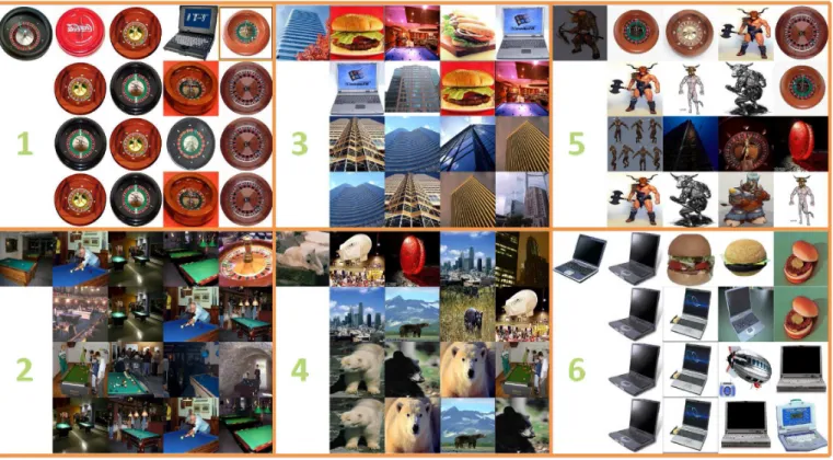
6.8 Qualitative Comparison
In the last experiment, we sample several query images, and compare the top ranked images retrieved by differ-ent methods. Fig. 4 shows the qualitative comparisons of six different query examples obtained by four dif-ferent algorithms, including “OASIS-Best”, “OKS-Best”, “OMKS-U” and “OMKS”. From the visual results, we observe that in general, “OKS-Best” retrieves more rel-evant images than “OASIS-Best”, as illustrated by the results for the first two queries. This result implies the importance of introducing nonlinear similarity functions in ranking. But at the same time, we notice that for all the other 4 queries, the results by “OKS-Best” are
0.1 0.2 0.3 0.4 0.5 0.6 0.7 0.8 0.9 1 0.16 0.18 0.2 0.22 0.24 0.26 0.28 0.3 RatioTrain m A P OASIS−Best OKS−Best OMKS−U OMKS−W OMKS 0.1 0.2 0.3 0.4 0.5 0.6 0.7 0.8 0.9 1 0.22 0.24 0.26 0.28 0.3 0.32 0.34 0.36 0.38 RatioTrain m A P OASIS−Best OKS−Best OMKS−U OMKS−W OMKS
(a) “Public” (b) “Caltech10”
Fig. 3. Evaluation ofRatioTrainon both “Public” and “Caltech10” data set. TABLE 3
Mean average precision and precision at top 1, 10 and 50 on the Caltech object data sets.
Caltech10 OMKS OKS-Best OASIS-Best OASIS-Ori Mean avg prec. 40±1.7 35±1.3 24±1.1 31±1.1
Top 1 prec. 59±1.8 49±3.3 35±3.4 45±2.1
Top 10 prec. 49±2.5 41±1.2 29±1.4 38±1.8
Top 50 prec. 27±1.3 25±1.0 20±0.5 23±0.3
Caltech20 OMKS OKS-Best OASIS-Best OASIS-Ori Mean avg prec. 31±0.6 25±0.7 20±0.5 19±0.7
Top 1 prec. 49±2.1 39±0.9 29±1.1 28±2.5
Top 10 prec. 39±0.8 31±1.0 24±0.9 23±1.1
Top 50 prec. 22±0.3 18±0.6 16±0.4 15±0.7
Caltech50 OMKS OKS-Best OASIS-Best OASIS-Ori Mean avg prec. 20±0.5 15±0.6 10±0.3 12±0.4
Top 1 prec. 36±1.5 26±1.5 16±1.5 20±0.6
Top 10 prec. 27±0.7 20±0.9 13±0.5 16±0.5
Top 50 prec. 15±0.2 12±0.3 9±0.1 10±0.3
not so perfect, which often returns irrelevant images similar to OASIS-Best. The result of query 3 and 4 indicates that “OMKS-U” tends to perform better than “OKS-Best”, validating the importance of incorporating multiple kernels built from diverse modalities. On the other hand, “OMKS-U” does not outperform “OKS-Best”. For example, for query 5, “OKS-Best” obtained 3 relevant images out of 4, while “OMKS-U” only obtained 1. Overall, OMKS overcomes the limitations of OMKS-U and is able to always find relevant images for all the queries, showing the significance of appropriately weighing individual kernels.
7
C
ONCLUSIONSThis paper addressed a fundamental problem of learning similarity functions for ranking images towards visual similarity search. To overcome the limitations of conven-tional distance metric learning techniques, we proposed a novel Online Multiple Kernel Similarity (OMKS) learn-ing scheme that can effectively improve image similarity
search by learning nonlinear proximity functions beyond conventional linear distance metric learning framework. By exploring the power of multiple kernels in combining multi-modal data, OMKS learns a much more flexible and powerful kernel-based proximity function to im-prove image similarity search in CBIR. We developed an efficient online learning algorithm and extensively evaluated the proposed algorithms for image similarity search on a number of public image databases. Our em-pirical results showed that OMKS significantly surpasses the state-of-the-art linear and nonlinear metric learning techniques for image similarity search. Despite being tested on image retrieval tasks, the proposed framework is rather generic for any multimedia retrieval tasks [50]. For future work, we plan to explore more applications and address other practical challenges of the proposed OMKS framework for large-scale applications, such as the convergence rate [51] and budget online learning issues [52].
A
CKNOWLEDGMENTSThis research was supported by Singapore MOE tier 1 grant (RG33/11).
R
EFERENCES[1] M. S. Lew, N. Sebe, C. Djeraba, and R. Jain, “Content-based multimedia information retrieval: State of the art and challenges,”
ACM Trans. Multimedia Comput. Commun. Appl., vol. 2, no. 1, pp. 1–19, 2006.
[2] Y. Jing and S. Baluja, “Visualrank: Applying pagerank to large-scale image search,”IEEE Trans. Pattern Anal. Mach. Intell., vol. 30, no. 11, pp. 1877–1890, 2008.
[3] D. Grangier and S. Bengio, “A discriminative kernel-based ap-proach to rank images from text queries,”IEEE Trans. Pattern Anal. Mach. Intell., vol. 30, no. 8, pp. 1371–1384, 2008.
[4] A. W. M. Smeulders, M. Worring, S. Santini, A. Gupta, and R. Jain, “Content-based image retrieval at the end of the early years,”
Fig. 4. Qualitative comparison of image similarity search results on the “Caltech10” database by different algorithms. For each block, the first image is the query, and the results from the first line to the fourth line represents “OASIS-Best”, “OKS-“OASIS-Best”, “OMKS-U” and “OMKS”, respectively. The category names for the queries are as follows: 1 (roulette wheel), 2 (billard), 3 (skyscraper), 4 (bear), 5 (minotaur), 6 (laptop).
[5] S. C. Hoi, W. Liu, M. R. Lyu, and W.-Y. Ma, “Learning dis-tance metrics with contextual constraints for image retrieval,” inProceedings of IEEE Conference on Computer Vision and Pattern Recognition, New York, US, Jun. 17–22 2006.
[6] R. Rahmani, S. A. Goldman, H. Zhang, S. R. Cholleti, and J. E. Fritts, “Localized content-based image retrieval,” IEEE Trans. Pattern Anal. Mach. Intell., vol. 30, no. 11, pp. 1902–1912, 2008. [7] S. Aksoy and R. M. Haralick, “Probabilistic vs. geometric
similar-ity measures for image retrieval,” inProceedings of IEEE Conference on Computer Vision and Pattern Recognition, 2000, pp. 2357–2362. [8] A. Qamra, Y. Meng, and E. Y. Chang, “Enhanced perceptual
distance functions and indexing for image replica recognition,”
IEEE Trans. Pattern Anal. Mach. Intell., vol. 27, no. 3, pp. 379–391, 2005.
[9] L. Si, R. Jin, S. C. Hoi, and M. R. Lyu, “Collaborative image re-trieval via regularized metric learning,”ACM Multimedia Systems Journal, vol. 12, no. 1, pp. 34–44, 2006.
[10] J.-E. Lee, R. Jin, and A. K. Jain, “Rank-based distance metric learning: An application to image retrieval,” inProceedings of IEEE Conference on Computer Vision and Pattern Recognition, Anchorage, AK, 2008.
[11] S. C. Hoi, W. Liu, and S.-F. Chang, “Semi-supervised distance metric learning for collaborative image retrieval and clustering,”
ACM Trans. Multimedia Comput. Commun. Appl., vol. 6, no. 3, pp. 18:1–18:26, Aug. 2010.
[12] R. Chatpatanasiri, T. Korsrilabutr, P. Tangchanachaianan, and B. Kijsirikul, “A new kernelization framework for mahalanobis distance learning algorithms,”Neurocomputing, vol. 73, no. 10-12, pp. 1570–1579, 2010.
[13] P. Jain, B. Kulis, J. V. Davis, and I. S. Dhillon, “Metric and kernel learning using a linear transformation,”Journal of Machine Learning Research, vol. 13, pp. 519–547, 2012.
[14] S. C. Hoi, J. Wang, and P. Zhao, LIBOL: A Library for Online Learning Algorithms, Nanyang Technological University, 2012. [Online]. Available: http://LIBOL.stevenhoi.org
[15] K. Crammer, O. Dekel, J. Keshet, S. Shalev-Shwartz, and Y. Singer,
“Online passive-aggressive algorithms,”Journal of Machine Learn-ing Research, vol. 7, pp. 551–585, 2006.
[16] S. C. Hoi, M. R. Lyu, and R. Jin, “A unified log-based relevance feedback scheme for image retrieval,”IEEE Trans. KDE, vol. 18, no. 4, pp. 509–204, 2006.
[17] P. Wu, S. C.-H. Hoi, P. Zhao, and Y. He, “Mining social images with distance metric learning for automated image tagging,” in
Proc. 4th ACM international conference on Web search and data mining (WSDM’11), Hong Kong, China, 2011, pp. 197–206.
[18] A. Bar-Hillel, T. Hertz, N. Shental, and D. Weinshall, “Learning a mahalanobis metric from equivalence constraints,” Journal of Machine Learning Research, vol. 6, pp. 937–965, 2005.
[19] E. P. Xing, A. Y. Ng, M. I. Jordan, and S. Russell, “Distance metric learning with application to clustering with side-information,” in
Advances in Neural Information Processing Systems, 2002.
[20] K. Weinberger, J. Blitzer, and L. Saul, “Distance metric learning for large margin nearest neighbor classification,” in Advances in Neural Information Processing Systems, 2006, pp. 1473–1480. [21] L. Wu, S. C. H. Hoi, R. Jin, J. Zhu, and N. Yu, “Distance metric
learning from uncertain side information with application to automated photo tagging,” in ACM Multimedia, 2009, pp. 135– 144.
[22] L. Yang, R. Jin, L. B. Mummert, R. Sukthankar, A. Goode, B. Zheng, S. C. H. Hoi, and M. Satyanarayanan, “A boosting framework for visuality-preserving distance metric learning and its application to medical image retrieval,” IEEE Trans. Pattern Anal. Mach. Intell., vol. 32, no. 1, pp. 30–44, 2010.
[23] A. Globerson and S. Roweis, “Metric learning by collapsing classes,” inAdvances in Neural Information Processing Systems, 2005. [24] A. Frome, Y. Singer, F. Sha, and J. Malik, “Learning globally-consistent local distance functions for shape-based image retrieval and classification,” inICCV, 2007, pp. 1–8.
[25] J. V. Davis, B. Kulis, P. Jain, S. Sra, and I. S. Dhillon, “Information-theoretic metric learning,” inICML, 2007, pp. 209–216.
online learning of image similarity through ranking,”Journal of Machine Learning Research, vol. 11, pp. 1109–1135, 2010.
[27] S. Tong and E. Chang, “Support vector machine active learning for image retrieval,” inProceedings of the ninth ACM international conference on Multimedia, Ottawa, Canada, 2001, pp. 107–118. [28] H. Chang and D.-Y. Yeung, “Kernel-based distance metric
learn-ing for content-based image retrieval,” Image Vision Comput., vol. 25, no. 5, pp. 695–703, 2007.
[29] D.-Y. Yeung and H. Chang, “A kernel approach for semisu-pervised metric learning,”IEEE Transactions on Neural Networks, vol. 18, no. 1, pp. 141–149, 2007.
[30] T. Hertz, A. Bar-Hillel, and D. Weinshall, “Learning a kernel function for classification with small training samples,” inICML, 2006, pp. 401–408.
[31] S. C. H. Hoi, R. Jin, and M. R. Lyu, “Learning nonparametric kernel matrices from pairwise constraints,” inProceedings of Inter-national Conference on Machine Learning, 2007, pp. 361–368. [32] J. Zhuang, I. W. Tsang, and S. C. H. Hoi, “A family of simple
non-parametric kernel learning algorithms,”J. Mach. Learn. Res., vol. 12, pp. 1313–1347, Jul. 2011.
[33] G. R. G. Lanckriet, N. Cristianini, P. Bartlett, L. E. Ghaoui, and M. I. Jordan, “Learning the kernel matrix with semidefinite programming,”Journal of Machine Learning Research, vol. 5, pp. 27–72, 2004.
[34] S. Sonnenburg, G. R¨atsch, C. Sch¨afer, and B. Sch ¨olkopf, “Large scale multiple kernel learning,”Journal of Machine Learning Re-search, vol. 7, pp. 1531–1565, 2006.
[35] Z. Xu, R. Jin, I. King, and M. R. Lyu, “An extended level method for efficient multiple kernel learning,” in Advances in Neural Information Processing Systems, 2008.
[36] A. Zien and C. S. Ong, “Multiclass multiple kernel learning,” in
Proceedings of International Conference on Machine Learning, Cor-valis, Oregon, 2007, pp. 1191–1198.
[37] S. Ji, L. Sun, R. Jin, and J. Ye, “Multi-label multiple kernel learning,” in Advances in Neural Information Processing Systems, 2008.
[38] M. Varma and B. R. Babu, “More generality in efficient multi-ple kernel learning,” inProceedings of International Conference on Machine Learning, 2009, pp. 1065–1072.
[39] S. V. N. Vishwanathan, Z. sun, N. Ampornpunt, and M. Varma, “Multiple kernel learning and the smo algorithm,” inNIPS, 2010, pp. 2361–2369.
[40] A. Jain, S. V. N. Vishwanathan, and M. Varma, “Spg-gmkl: Generalized multiple kernel learning with a million kernels,” in
Proceedings of the ACM SIGKDD Conference on Knowledge Discovery and Data Mining, August 2012.
[41] R. Jin, S. C. H. Hoi, and T. Yang, “Online multiple kernel learning: Algorithms and mistake bounds,” inALT, 2010, pp. 390–404. [42] S. C. Hoi, R. Jin, P. Zhao, and T. Yang, “Online multiple kernel
classification,”Machine Learning, vol. 90, no. 2, pp. 289–316, 2013. [43] M. Varma and D. Ray, “Learning the discriminative power-invariance trade-off,” inProceedings of IEEE International Conference on Computer Vision, 2007, pp. 1–8.
[44] A. Vedaldi, V. Gulshan, M. Varma, and A. Zisserman, “Multiple kernels for object detection,” inICCV, 2009, pp. 606–613. [45] A. Quattoni and A. Torralba, “Recognizing indoor scenes,” in
Proceedings of IEEE Conference on Computer Vision and Pattern Recognition, 2009, pp. 413–420.
[46] G. Griffin, A. Holub, and P. Perona, “Caltech-256 object category dataset,” California Institute of Technology, Tech. Rep. 7694, 2007. [47] J. Philbin, O. Chum, M. Isard, J. Sivic, and A. Zisserman, “Object retrieval with large vocabularies and fast spatial matching,” in
Proceedings of the IEEE Conference on Computer Vision and Pattern Recognition, 2007.
[48] A. Bar-Hillel, T. Hertz, N. Shental, and D. Weinshall, “Learning distance functions using equivalence relations,” inProceedings of International Conference on Machine Learning, 2003, pp. 11–18. [49] I. W. Tsang, P. ming Cheung, and J. T. Kwok, “Kernel relevant
component analysis for distance metric learning,” inIEEE Inter-national Joint Conference on Neural Networks (IJCNN), 2005, pp. 954– 959.
[50] S. C. Hoi and M. R. Lyu, “A multimodal and multilevel ranking scheme for large-scale video retrieval,”Multimedia, IEEE Transac-tions on, vol. 10, no. 4, pp. 607–619, 2008.
[51] P. Zhao, S. C. Hoi, and R. Jin, “Double updating online learning.”
Journal of Machine Learning Research, vol. 12, pp. 1587–1615, 2011.
[52] P. Zhao, J. Wang, P. Wu, R. Jin, and S. C. Hoi, “Fast bounded on-line gradient descent algorithms for scalable kernel-based onon-line learning,” 2012.
Hao Xia is currently a PhD candidate in the
School of Computer Engineering at the Nanyang Technological University, Singapore. He re-ceived his bachelor degree from Tsinghua Uni-versity, Beijing, P.R. China, in 2008. His research interests are statistical machine learning, data mining, and multimedia information retrieval.
Steven C. H. Hoi is an Associate
Profes-sor of the School of Computer Engineering at Nanyang Technological University, Singapore. He received his Bachelor degree from Tsinghua University, P.R. China, in 2002, and his Ph.D de-gree in computer science and engineering from The Chinese University of Hong Kong, in 2006. His research interests are machine learning and data mining and their applications to multimedia information retrieval (image and video retrieval), social media and web mining, and computational finance, etc. He has published over 100 referred papers in top con-ferences and journals in related areas. He has served as general co-chair for ACM SIGMM Workshops on Social Media (WSM’09, WSM’10, WSM’11), program co-chair for the fourth Asian Conference on Machine Learning (ACML’12), book editor for “Social Media Modeling and Com-puting”, guest editor for ACM Transactions on Intelligent Systems and Technology (ACM TIST), technical PC member for many international conferences, and external reviewer for many top journals and worldwide funding agencies, including NSF in US and RGC in Hong Kong. He is a member of IEEE and ACM.
Rong Jin is currently an Associate Professor
in the department of Computer Science and Engineering at Michigan State University. He received his Ph.D. degree in Computer Science from Carnegie Mellon University, 2003. His re-search interests are statistical learning and its application to large-scale information manage-ment, including web text retrieval, content-based image retrieval, gene regulatory network recon-struction, neuron data analysis, and visual object recognition.
Peilin Zhao is currently a PhD candidate in
the School of Computer Engineering at the Nanyang Technological University, Singapore. He received his bachelor degree from Zhejiang University, Hangzhou, P.R. China, in 2008. His research interests are statistical machine learn-ing, and data mining.