Anomaly Detection
Alexander T. M. Fisch BA, MMath, MRes
Submitted for the degree of Doctor of
Philosophy at Lancaster University.
Anomaly detection is of increasing importance in the data rich world of today. It can be applied to a broad range of challenges ranging from fault detection to fraud preven-tion and cyber-security. Many of these applicapreven-tion require algorithms which are very scalable, as well as accurate, due to large data volumes and/or limited computational resources.
This thesis contributes three novel approaches to the field of anomaly detection. The first contribution, Collective And Point Anomalies (CAPA) detects and distin-guishes between both collective and point anomalies in linear time. The second contri-bution, MultiVariate Collective And Point Anomalies (MVCAPA) extends CAPA to the multivariate setting. The third contribution is a novel particle based kalman filter which detects and distinguished between additive outliers and innovative outliers.
First and foremost, I would like to thank my Lancaster supervisors Paul Fearnhead and Idris Eckley for their help and guidance throughout my PhD. I am especially grateful for their willingness to wade through the rather long proofs. I would also like to thank Dan Grose, for helping with packaging up the various methods developed as part of this thesis. Thanks also to the wider time-series, changepoint, and com-putational stats community for stimulating discussions. Thanks also to my external examiner Jean-Philippe Vert and my internal examiner Azadeh Khaleghi for a very stimulating and thought provoking viva.
I am very grateful to the STOR-i CDT, EPSRC, and British Telecommunications PLC (BT) for funding this thesis. BT and its employees, especially Trevor Burbridge, Kjeld Jensen, and David Yearling, have also been very helpful by providing data examples and helpful discussions which have inspired much of this work. I am also very grateful for having been given the opportunity to visit their office on several occasions to get my hands dirty on real data.
On a more personal level, I would like to thank my wife, Sol`ene, for bearing with me – and with the “brilliant ideas” that seem to come at 1am. I would also like to
thank the wider STOR-i and StatScale community for providing such a pleasant work environment. AMDG.
I declare that the work in this thesis has been done by myself and has not been submitted elsewhere for the award of any other degree.
Chapter 3 is currently under review with Data Mining and Knowledge Discovery. Chapter 4 is currently under review with the Journal of Computational and Graph-ical Statistics.
Chapter 5 is currently under review with IEEE Transactions on Signal Processing.
Alexander T. M. Fisch
Abstract I
Acknowledgements II
Declaration IV
Contents XI
List of Figures XIII
List of Tables XIV
1 Introduction 1
2 Background and Literature Review 4
2.1 Robust Statistics . . . 4
2.1.1 Definitions Around Robustness . . . 5
2.1.2 M-Estimators . . . 7
2.2 Kalman Filtering Approaches . . . 8
2.2.1 The Classical Kalman Filter . . . 9
2.2.2 Variational Bayes and t-Distributed Noise . . . 10
2.2.3 Huberisation and Robust Statistics . . . 12
2.2.4 Other Approaches . . . 13
2.3 Changepoint Approaches . . . 13
2.3.1 Univariate Changepoint Models . . . 14
2.3.2 Epidemic Changepoint Models for Univariate Data . . . 20
2.3.3 Epidemic Changepoint Models for Multivariate Data . . . 24
3 Collective And Point Anomalies 30 3.1 Introduction . . . 30
3.2 A Modelling Framework for Collective Anomalies . . . 35
3.3 Estimation of Collective and Point Anomalies . . . 38
3.4 Theory for Joint Changes in Mean and Variance . . . 41
3.4.1 Consistency of Classical Changepoint Detection . . . 41
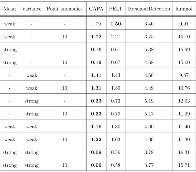
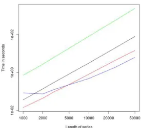
3.4.2 Consistency of CAPA . . . 44 3.4.3 Penalties . . . 47 3.5 Simulation Study . . . 49 3.5.1 ROC . . . 50 3.5.2 Precision . . . 52 3.5.3 Runtime . . . 54 3.6 Applications . . . 55
3.6.1 Kepler Light Curve Data . . . 58
4 Multivariate Collective And Point Anomalies 62
4.1 Introduction . . . 62
4.2 Model and Inference for a Single Collective Anomaly . . . 67
4.2.1 Penalised Cost Approach . . . 67
4.2.2 Choosing Appropriate Penalties . . . 70
4.2.3 Results on Power . . . 74
4.3 Inference for Multiple Anomalies . . . 76
4.4 Computation . . . 78
4.5 Accuracy of Detecting and Locating Multiple Collective Anomalies . 80 4.6 Incorporating Lags . . . 83
4.6.1 Extending the Test Statistic . . . 83
4.6.2 Result on Power . . . 85
4.6.3 Computational Considerations . . . 86
4.7 Simulation Study . . . 87
4.7.1 ROC Curves . . . 89
4.7.2 Precision . . . 92
4.8 Detecting Copy Number Variation . . . 94
5 Innovative And Additive Outlier Robust Kalman Filtering 97 5.1 Introduction And Literature Review . . . 97
5.2 Model And Examples . . . 102
5.3 Particle Filter . . . 105
5.3.2 Choices of Parameters . . . 111
5.3.3 Example 1 - revisited . . . 112
5.4 Particle Filter With Back-Sampling – CE-BASS . . . 113
5.4.1 Back-Sampling Particles Using the Last k+ 1 Observations . . 113
5.4.2 Example . . . 118
5.5 Simulations . . . 119
5.6 Application . . . 123
5.6.1 Machine Temperature Data . . . 123
5.6.2 Router Data . . . 125
6 Conclusions And Further Research 129 A CAPA 131 A.1 Pseudocode for CAPA . . . 131
A.2 Proofs of Propositions and Theorems . . . 134
A.2.1 Proof of Proposition 1 . . . 134
A.2.2 Proof of Proposition 2 . . . 134
A.2.3 Proof of Proposition 3 . . . 137
A.2.4 Proof of Theorem 1 . . . 139
A.2.5 Proof of Theorem 2 . . . 146
A.3 Additional Lemmata . . . 152
A.4 Proofs of Main Lemmata . . . 154
A.4.1 Proof of Lemma 1 . . . 154
A.4.3 Proof of Lemma 3 . . . 157
A.4.4 Proof of Lemma 4 . . . 158
A.4.5 Proof of Lemma 5 . . . 159
A.4.6 Proof of Lemma 6 . . . 160
A.4.7 Proof of Lemma 7 . . . 160
A.4.8 Proof of Lemma 8 . . . 161
A.4.9 Proof of Lemma 9 . . . 162
A.4.10 Proof of Lemma 10 . . . 163
A.4.11 Proof of Lemma 11 . . . 163
A.5 Further Simulation Study Results . . . 166
A.6 Application of CAPA to Further Stars . . . 169
B MVCAPA 172 B.1 Additional Theoretical Results . . . 172
B.1.1 Pruning Without Lags . . . 172
B.1.2 Bounds on Lagged Savings . . . 173
B.1.3 Pruning the Dynamic Programme in the Presence of Lags . . 173
B.2 Proofs for Theorems and Propositions . . . 175
B.2.1 Proof of Proposition 4 . . . 175
B.2.2 Proof of Proposition 5 . . . 177
B.2.3 Proof of Proposition 6 . . . 184
B.2.4 Proof of Propositions 17 and 19 . . . 184
B.2.6 Proof of Proposition 7 . . . 186
B.2.7 Proof of Proposition 8 . . . 186
B.2.8 Proof of Theorem 3 . . . 187
B.3 Proofs for Lemmata . . . 212
B.3.1 Proof of Lemma 14 . . . 212 B.3.2 Proof of Lemma 15 . . . 212 B.3.3 Proof of Lemma 16 . . . 215 B.3.4 Proof of Lemma 17 . . . 215 B.3.5 Proof of Lemma 18 . . . 217 B.3.6 Proof of Lemma 19 . . . 217 B.3.7 Proof of Lemma 20 . . . 218 B.3.8 Proof of Lemma 21 . . . 219 B.3.9 Proof of Lemma 22 . . . 222 B.3.10 Proof of Lemma 23 . . . 222 B.3.11 Proof of Lemma 24 . . . 223 B.3.12 Proof of Lemma 25 . . . 224 B.3.13 Proof of Lemma 26 . . . 225 B.3.14 Proof of Lemma 27 . . . 226 B.3.15 Proof of Lemma 28 . . . 227 B.3.16 Proof of Lemma 29 . . . 227 B.3.17 Proof of Lemma 30 . . . 229 B.3.18 Proof of Lemma 31 . . . 229 B.3.19 Proof of Lemma 32 . . . 230
B.3.20 Proof of Lemma 33 . . . 233
B.3.21 Proof of Lemma 34 . . . 233
B.3.22 Proof of Lemma 35 . . . 233
B.3.23 Proof of Lemma 36 . . . 233
B.4 Further Simulations And Tables . . . 238
B.5 Pseudocode . . . 246
C CE-BASS 251 C.1 Theorems and Derivations . . . 251
C.1.1 Theorem 5 . . . 251 C.1.2 Theorem 6 . . . 253 C.1.3 Theorem 7 . . . 254 C.1.4 Proof of Theorem 4 . . . 254 C.1.5 Theorem 8 . . . 256 C.2 Additional Simulations . . . 256 C.3 Complete pseudocode . . . 256 Bibliography 265
2.3.1 An example time series with K = 3 changes in mean. . . 15
2.3.2 An example time series with K = 2 epidemic changes in mean. . . 21
2.3.3 An example multivariate time series with K = 2 epidemic changes in mean. . . 25
3.5.1 Data examples and ROC curves for changes in mean. . . 51
3.5.2 log-log-plot of the runtime . . . 54
3.6.1 Light curve of Kepler 1132 . . . 56
3.6.2 CAPA applied to the light curve of Kepler 1132. . . 56
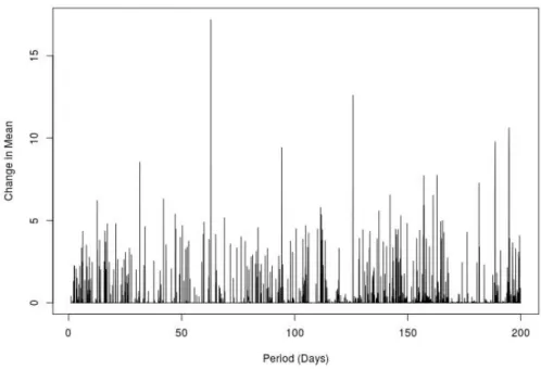
3.6.3 The strongest change in mean detected by CAPA for the lightcurve of Kepler 1132 . . . 57
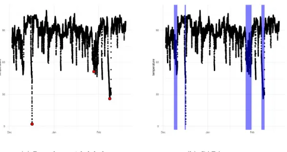
3.6.4 Machine temperature data. . . 60
4.1.1 A time series withK = 2 collective anomalies. . . 64
4.2.1 A comparison of the 3 penalty regimes. . . 72
4.7.1 Example series and ROC curves. . . 90
5.2.1 Two examples of time series which are realisations of outlier infested
Kalman models. . . 103
5.3.1 Robust particle filter output at various times. . . 112
5.4.1 Robust particle filter output at various times. . . 118
5.5.1 Average predictive log-likelihood of the five filters. . . 120
5.6.1 Machine temperature dataset. . . 124
5.6.2 CE-BASS applied to 9 days of de-seasonalised router data. . . 126
A.5.1Data examples and ROC curves for changes in variance. . . 167
A.5.2Data examples and ROC curves for joint changes in mean and variance. 168 A.6.1The strongest change in mean detected by CAPA for the lightcurves of five stars with known exoplanets . . . 170
A.6.2Five stars orbited by known exoplanets. . . 171
B.2.1Examples of the four ways a fitted partition can be outside the set of good partitions. . . 188
B.4.1Example series and ROC curves for setting 1. . . 239
B.4.2Example series and ROC curves for setting 2. . . 240
B.4.3Example series and ROC curves for setting 3. . . 241
B.4.4Example series and ROC curves for setting 4. . . 242
B.4.5Example series and ROC curves for setting 1. . . 243
B.4.6Example series and ROC curves for setting 3. . . 244
B.4.7Analysis of Chromosome 6. . . 245
3.5.1 Precision of true positives. . . 53
4.7.1 Precision of true positives. . . 93 4.8.1 A comparison between PASS and MVCAPA for chromosome 16 . . . 96
Introduction
Anomaly detection is an area of considerable importance and has been subject to increasing attention in recent years. This is due to the wide range of applications the field lends itself to. Examples include fault detection (Theissler, 2017; Zhao et al., 2018), fraud prevention (Ahmed et al., 2016), and cyber security (Goh et al., 2017). The ubiquity of sensors and the emergence of the Internet of Things (IoT) has lead to the detection of anomalies in streaming data to emerge as a new and critical challenge. One important aspect of anomalies is that they can come in different guises. One classification was offered by Chandola et al. (2009) who distinguish between global, contextual, and collective anomalies. Here global anomalies are single points which fall outside the general pattern of the data while contextual anomalies fall outside their local data pattern. Collective anomalies on the other hand are defined to be a sequence of observations which are not necessarily anomalous by themselves but together form an anomalous pattern. The Kalman filtering literature similarly distinguishes between punctual anomalies called additive outliers which affect the observations only and
persisting anomalies called innovative outliers which affect the system (Ruckdeschel et al., 2014).
This thesis introduces novel statistical methods for detecting and distinguishing between different types of anomalies in a computationally efficient manner. All al-gorithms have been inspired by anomalies observed in telecommunications network data.
The remainder of the thesis is organised as follows: We begin by reviewing relevant background in Chapter 2. The focus of this chapter will lie on robust statistics, Kalman filtering and changepoint methods.
In Chapter 3, we propose a new epidemic changepoint based algorithm which can detect and distinguish between collective an point anomalies in empirically linear time. We call the algorithm Collective And Point Anomalies (CAPA), theoretically prove its consistency, empirically evaluate it against competing methods, and apply it to monitoring machine temperature data and to exoplanet detection.
We propose extension of CAPA to the multivariate setting, which we call multivari-ate CAPA (MVCAPA), in Chapter 4. Crucially, the proposed methodology allows for related anomalies in different components to have imperfect alignment across time. We theoretically show MVCAPA’s consistency and that it is able to optimally de-tect sparse anomalies, affecting only a few components, as well as dense anomalies, affecting a large subset of components.
A novel Kalman filter which is robust to both additive and innovative outliers is proposed in chapter 5. The proposed methodology, which we call Computationally Efficient Bayesian Anomaly detection by Sequential Sampling (CE-BASS) is fully
online, very scalable, and shown to compare favourably with other robust filters. CE-BASS is applied to both real router data and a benchmark dataset.
We discuss our contribution to the literature as well as potential areas of further research in Chapter 6.
Background and Literature Review
In this chapter, we review some of the background literature relevant to this thesis. We will begin by reviewing the pertinent definitions and concepts in robust statistics in Section 2.1 before reviewing the robust Kalman Filter literature in Section 2.2 and the changepoint literature in 2.3. We purposefully omit reviewing the vast range of anomaly detection approaches proposed by the machine learning and computer science community and instead refer to the excellent reviews which can be found in Chandola et al. (2009) and Pimentel et al. (2014), as well as the more recent papers by Lavin and Ahmad (2015), Talagala et al. (2019), Ahmad et al. (2017), and references therein.
2.1
Robust Statistics
When the distribution of the typical data is known, detecting anomalies becomes almost trivial. However, inferring the distribution of the typical data from a data
set which is potentially polluted by anomalies is difficult as outliers can significantly affect the inference procedure. Take the sample mean for example: A single outlier has the potential of irreversibly polluting this statistic, hence making it useless for the purpose of detecting anomalies. Other commonly used statistics such as the sample variance, regression coefficients, sample covariance matrices, etc. are equally vulnerable to outliers.
Observations like the above have motivated the field of robust statistics. Robust statistics aim to bound the influence any single data point can have on the statistic while equally trying to achieve an efficiency which is close to that of maximum like-lihood estimators. We will review the key concepts of the field in this section, as it provides important background to subsequent sections and chapters.
2.1.1
Definitions Around Robustness
The main concept in robustness is the influence function, first introduced by Hampel (1968). For a given statistic,T(), which is a functional mapping a cumulative density functionF() to a scalar, the influence function is defined via the Gateaux derivative
IF(x, F) = lim →0
T((1−)F +4x)−T(F)
. (2.1.1)
Here, 4x(y) =I(y≥x) denotes the CDF of point mass at x. It captures how much deviations from the assumed distribution can affect the statistic. A statistic is said to be robust if the influence function is bounded (Hampel et al., 1986).
For example, the mean is defined by the functionalT(G) =R xdG(x). For a distri-butionF with mean µthe influence function is therefore given byx−µ. Conversely,
the median is defined by the functionalT(G) = G−1(1/2). Its influence function for a distribution with PDF f and median m is therefore
1
f(m)(I(x < m)− 1
2). (2.1.2)
This confirms the intuition that the mean is not a robust statistic whilst the median is robust.
Another important metric in robust statistics is the breakdown point which mea-sures the proportion of data that can be anomalous whilst guaranteeing that the difference between the statistic on the polluted data and the statistic on the unpol-luted data is finite. Formally it can be defined as the largestγ such that
sup G,<γ
|T((1−)F +G)−T(F)|<∞.
It can be shown to be 0 for the mean and 12 for the median. The median therefore achieves the theoretical maximal breakdown point. Indeed, it can be shown that the breakdown point must be less or equal to 12 – otherwise there would be identifiability issues (Hampel et al., 1986).
Finally, the asymptotic efficiency is an important metric. Robust estimators achieve robustness by ignoring or down-weighting parts of the data. They are therefore less efficient than the maximum likelihood estimator (MLE). This is captured by the asymptotic efficiency which is defined as the asymptotic variance of the MLE divided by that of the robust estimator. For instance, the median achieves and asymptotic efficiency of 2/π for normal data (Hampel et al., 1986).
2.1.2
M
-Estimators
The median mentioned in the previous section is an example of anL-estimator, where
L is short for location. Other examples of such L-estimators are the α-trimmed mean which neglects theα% of lowest and highest observations. L-estimators for the variance also exist, such as the inter-quartile range, the α-trimmed variance, or the median absolute deviation (Hampel et al., 1986).
However, a different class of estimators calledM-estimators, going back to Huber (1964b), tend to be preferred due to their better efficiency (Jureˇckov´a and Picek, 2005). M-estimators are obtained through a minimisation problem: For a suitable cost function ρ(·,·), the M-estimator of a parameter θ is obtained from observations
x1, ..., xn by minimising n X i=1 ρ(xi, θ) !
with respect to θ. This can be viewed as a generalisation of the MLE since taking
ρ(·,·) to be the negative log-likelihood recovers the MLE.
A range of cost functionsρ() has been proposed with the aim of achieving robust-ness. One such function is Tukey’s bi-weight loss (Tukey, 1960), defined as
ρ(xi, θ) = (xi−θ)2 |xi−θ|< h, h2 |x i−θ| ≥h,
which can be shown to bound the influence function at h. Here, the threshold pa-rameterhgoverns the trade-off between robustness and efficiency – the higher h, the more efficient the estimate becomes, the lower h, the more robust.
Another robust loss function is Huber loss (Huber, 1964a) which is defined as: ρ(xi, θ) = (xi−θ)2 |xi−θ|< h, 2h|xi−θ| −h2 |xi−θ| ≥h.
It can be shown to bound the influence function ath. Furthermore, it provides a trade-off between robustness and efficiency which is in some sense pareto-optimal. Indeed, Hampel (1968) showed that Huberisation, i.e. truncating the influence function of an MLE achieves maximal efficiency for a given breakdown point.
Other commonly used robust loss functions include the Dynamic Covariance Scal-ing (Agarwal et al., 2013) and the log-likelihood of the t-distribution distribution (Agamennoni et al., 2012).
2.2
Kalman Filtering Approaches
An important challenge in many anomaly detection applications is that sequential or online processing of time series data is often a requirement. The Kalman filter first proposed by Kalman (1960) uses a latent variable model which provides a conve-nient way of processing new observations at a fixed computational cost. Furthermore, having processed observations Y1, ....,Yn, the Kalman filter can return a mean and variance estimate forYn+1, making it, in principle, very well suited for anomaly detec-tion: A Mahalanobis distance can be computed and an anomaly declared if it exceeds a predefined quantile of theχ2-distribution. However, the Gaussian noise model used by the classical Kalman filter makes it vulnerable to outliers. A range of outlier robust Kalman filters, more suitable to anomaly detection, has therefore been proposed.
We will begin this section by reviewing the Kalman filter and discuss the two types of anomalies which can affect it. We will then discuss the most common approaches aimed at robustifying the Kalman filter namely filters which uset-distributed noise in conjunction with Variational Bayes (VB), filters which use Huberisation, and filters which use heavy tailed noise in conjunction with other methods to maintain approx-imations to the posterior.
2.2.1
The Classical Kalman Filter
The Kalman filter goes back to the seminal paper Kalman (1960). It considers a model in which observations Y1, ...,Yn are underpinned by hidden variables X1, ...,Xn in the following manner:
Yt=CXt+ηt Xt =AXt−1+t.
Here the noise processesηt i.i.d
∼ N(0,R) and t i.i.d
∼ N(0,Q) are independent for t≥1 and a priorX0 ∼N(µ0,Σ0) is put on the initial state.
The main feature of the Kalman filter is that it allows for online updates of the hid-den state. WhenXt|Yt, ....,Y1 ∼N(µt,Σt), it can be shown thatXt+1|Yt+1, ....,Y1 ∼
µt and Σt through the update equations ˆ µ=Aµt ˆ Σ=AΣtAT +Q z=Yt−Cµˆ K=CΣCˆ T +R −1 CΣˆ µt+1= ˆµ+KTz Σt+1= (I−KCT) ˆΣ. (2.2.1)
As mentioned in the introduction to this section, the Gaussian noise model used by the Kalman filter make it very vulnerable to outliers. One particular challenge is that two types of outliers can occur: additive outliers (Ruckdeschel et al., 2014), sometimes called observational outliers (Gandhi and Mili, 2009), affect the processηt. Their impact is limited to just one time point. Conversely, innovative (Ruckdeschel et al., 2014), or process (Huang et al., 2017) outliers, affect the process t. Their impact can potentially affect many observations to come. Robustness against just one of these two types of outliers typically make the filter more vulnerable to the other. For instance, additive outlier robust filters tend to update the hidden variables even less than the classical Kalman filter when encountering an innovative outlier (Ruckdeschel et al., 2014).
2.2.2
Variational Bayes and
t-Distributed Noise
A number of filters which achieve robustness to outliers by assuming t-distributed noise processes ηt and/or t has been proposed. For example, Agamennoni et al.
(2011) assumed t-distributed noise ηt to achieve robustness against additive out-liers. The authors use the conditional noise model ηt
i.i.d
∼ N(0,St), where S−t1 ∼
W(R−1/s, s). Here, W() denotes the Wishart distribution, which generalises the Gamma distribution to the multivariate setting. Whilst this model achieves robust-ness to additive outliers, there is no longer a tractable filter. Indeed, given a Gaussian prior Xt|Yt, ....,Y1 ∼ N(µt,Σt), the posterior Xt+1|Yt+1, ....,Y1 is no longer Gaus-sian.
Variational Bayes is often used to obtain a Gaussian approximation to the poste-rior. It finds the Normal distribution which minimises the Kullback-Leibler divergence with the posterior distribution. In conjunction with t-distributed noise, this is often relatively easy to do. For example, in the model considered by Agamennoni et al. (2011), the posterior can be obtained by initialisingS=R and iterating the Kalman like equations K=CΣCˆ T +S −1 CΣˆ µt+1 = ˆµ+KTz Σt+1 =KSKT + (I−KCT) ˆΣ(I−CKT) S= sR+ (Yt−Cµt+1)(Yt−Cµt+1) T +CΣ t+1CT s+ 1
until convergence. Similar ideas can be found in the filters proposed by Ting et al. (2007), also robust to additive outliers and Huang et al. (2017, 2019) who propose filters which are robust against both additive and innovative outliers.
2.2.3
Huberisation and Robust Statistics
Approaches inspired by robust statistics can be used to truncate the effect of individual observations to achieve robustness against additive outliers or to truncate the effect of the prior state to achieve robustness against innovative outliers.
An example of such a filter is the additive outlier robust filter using Huberisation proposed by Ruckdeschel et al. (2014). The authors replace
µt+1 = ˆµ+KTz
in Equation (2.2.1) by
µt+1 = ˆµ+H(KTz, b).
HereH(x, b) denotes x Huberised at level b, which is formally defined as
H(x, b) =xmin 1, b x .
In the same paper, Ruckdeschel et al. (2014) also show that robustness against innovative outliers can be achieved if Cis invertible by replacing
µt+1 = ˆµ+KTz
in Equation (2.2.1) by
µt+1 = ˆµ+C−1 z−H( I−CKT
z, b).
Similar approaches, inspired by robust statistics were used by (Gandhi and Mili, 2009) for robustness against additive and innovative outliers and Chang et al. (2013) for robustness against additive outliers.
2.2.4
Other Approaches
Other approaches using heavy tailed noise and approximating the posterior have also been proposed. Kitagawa (1987) for instance proposed an approach which consists of using splines to approximate the posterior distribution at each time point. The proposed methodology is shown to be able to deal with both additive and innovative outliers but scales poorly with the dimensionality of the problem.
Particle filtering (Fearnhead and K¨unsch, 2018) to approximate the distribution ofxt has also been proposed. Gordon et al. (1993) proposed to sample from the noise at each time point and give particles weight proportional to the likelihood. However, such approaches are not computationally robust against outliers, as noted by Chang (2014): As outliers become stronger it is less and less likely that an appropriate particle will be sampled. Some particle filters offering computational robustness to specific models (Fearnhead and Clifford, 2003) and to additive outliers (Xu et al., 2013) have therefore been proposed. The filter by Harrison and Stevens (1976) is also often mentioned as being robust to both types of outliers. However, it uses a Gaussian mixture model and is therefore not robust to outliers.
2.3
Changepoint Approaches
Observing that our world is ever-changing, the ancient Greek philosopher Heraclitus claimed that “No man ever steps in the same river twice, for it’s not the same river and he’s not the same man”. It can be assumed that Heraclitus would object to time series being modelled as stationary, on similar grounds. Indeed, data generating
mechanisms often change. One approach of modelling this non-stationarity is via changepoints.
The literature considers two main types of changepoint models: Classical point models, typically only referred to as changepoint models, and epidemic change-point models. The classical changechange-point model, first considered by Page (1954), as-sumes that there exists a set of time-points at which the data-generating mechanism changes. The epidemic changepoint model, going back to Levin and Kline (1985) according to Yao (1993), assumes that the data follows some typical distribution for most of the time except during certain windows in which it behaves differently. These epidemic changes provide a natural model for collective anomalies.
In what follows, we will begin by reviewing the classical changepoint model as well as some some of the main approaches for changepoint inference in Section 2.3.1. This is mostly for background as the main focus of this section lies on the closely related epidemic changepoint detection problem. In Section 2.3.2, we will then review current approaches for the detection of univariate epidemic changepoints. This will be followed by a discussion of multivariate approaches in Section 2.3.3. For simplicity of exposition, we will focus on the change in mean setting, the frameworks being more general.
2.3.1
Univariate Changepoint Models
Consider a univariate time seriesx1, ..., xn. It is said to obey the classical changepoint model if there exists a set of changes τ = {t0, ..., tK+1}, where 0 = t0 < t1... < tK ≤
Figure 2.3.1: An example time series with K = 3 changes in mean. The first change occurs att1 = 100, the second at t2 = 250, and the third at t3 = 350.
tK+1 =n, such that xt ∼ M0 t0 < t≤t1, .. . MK tK < t≤tK+1, 1≤t ≤n.
HereMk denotes the model obeyed by the data before the kth changepoint. Setting
Mk = N(µk, σ2) gives rise to the change in mean problem with Gaussian noise. This setting has received a considerable amount of attention (Killick et al., 2012; Fryzlewicz, 2014) and will be the main focus of the remainder of this section for simplicity of exposition.
Detecting a Single Change
We will begin by reviewing the case in which at most one change (AMOC) is present. This is because approaches for the AMOC setting can be extended to multiple changes
using the Binary Segmentation algorithm described in the next section. In the AMOC setting, it is of interest to test the null hypothesis of a stationary mean
H0 :µ1 =...=µn,
against the alternative hypothesis
H1 :∃T : 0≤T ≤n, µ1 =...=µT 6=µT+1 =...=µn, which states that a change is present at some time T.
If a single time point,T, had to be investigated, using a log-likelihood ratio statistic would be a natural choice. It can be shown that this statistic is the square of the following cumulative sum (CUSUM) statistic
ST = r n−T nT T X t=1 xt− s T n(n−T) n X t=T+1 xt .
It is therefore natural to compute this statistic for all candidate integers 1≤T ≤n−1. If max (ST2) then exceeds a threshold λ a change at time argmax (ST2) is inferred. Otherwise, no changepoint is returned. Suitable choices forλare discussed in Section 2.3.1. It should be noted that this approach is not restricted to the change in mean setting. It can be extended to any type of change provided an appropriate likelihood ratio tests exists.
Binary Segmentation Approaches
Binary Segmentation, introduced by Scott and Knott (1974) can be used to extend any AMOC changepoint method to infer multiple changepoints. The idea behind Binary Segmentation consists of repeatedly applying an AMOC procedure to segments between inferred changepoints. The algorithm can be summarised as follows:
1. Apply the AMOC procedure to the data x1,...,xn and obtain candidate change-point change-points T.
2. If the statistic does not exceed the threshold λ stop. Otherwise consider T to be a changepoint
3. Repeat the above procedure on the sequencesx1,...,xT and xT+1,...,xn
Binary segmentation is computationally very efficient. Indeed, its computational complexity isO(nlog(n)). However, it has been shown to yield unsatisfactory results even in the absence of any noise in certain settings (Fryzlewicz, 2014). This has lead to the development of derived methods such as Wild Binary Segmentation (Fryzlewicz, 2014).
Penalised Cost Approaches
An alternative approach to Binary Segmentation consists of minimising a penalised cost (Killick et al., 2012; Jackson et al., 2005). In this approach, each segment of data between two inferred changepoints is allocated a cost, such as twice the negative log-likelihood evaluated at the segment’s MLE. Every additional changepoint introduced typically reduces the total cost and therefore incurs a penaltyβ to avoid over-fitting. The number of changepoints ˆK and changepoints t1, ..., tKˆ are then inferred by min-imising the penalised cost:
ˆ K X i=0 C x(ti+1):ti+1 + ˆKβ
The cost functionC is chosen in the light of the model considered. For the change-in mean case, for example, it is natural to use the residual sum of squares, i.e.
C(xa:b) = min µ b X i=a (xi−µ)2 ! = b X i=a x2i −(b−a+ 1) (¯xa:b)2. It should be noted that for a≤b < c
C(xa:c)− C(xa:b) +C x(b+1):c = s c−b (b−a+ 1)(c−a+ 1) T X t=1 xt− s c−a+ 1 (b−a+ 1)(c−b) c X t=b+1 xt !2
holds, i.e. that the reduction in cost obtained by splitting a segment is equal to the CUSUM statistic. Consequently, Binary Segmentation can be viewed as a greedy heuristic for minimising the penalised cost.
Efficient Inference for Penalised Cost Approaches
The penalised cost introduced in the previous section can be minimised exactly via Optimal Partitioning (OP) introduced by Jackson et al. (2005). To this end,C(m) is defined to be the cost of the optimal partition of all observations up to and including the mth one. The following recursive relationship then holds:
C(m) = min
1≤k≤m(C(k−1) +C(xk:m) +β).
In the above, the optimalk represents the optimal changepoint preceding m, condi-tional on m being a changepoint. Solving the above dynamic programme therefore returns the optimal partition.
It can be shown that solving the full dynamic programme is at leastO(n2) (Killick et al., 2012). However, Killick et al. (2012) showed that the solution space of the dynamic programme can be pruned thereby reducing the computational cost. Indeed
the authors showed that if the cost function is such that
C(xa:c)≥ C(xa:b) +C x(b+1):c
, ∀a≤b < c
i.e. such that adding an additional change does not reduce the cost, then if
C(k−1) +C(xk:m)> C(m) +β
holds for some k ≤ m then k can be disregarded for all future steps of the dynamic programme, without affecting the cost optimality of the returned partition. Kil-lick et al. (2012) use this observation in their algorithm Pruned Exact Linear Time (PELT), to solve a pruned version of the dynamic programme considered by OP. The authors showed that PELT can be significantly faster than OP, especially when mul-tiple changepoints are present and have a computational cost which is as low asO(n) when the number of changes increases linearly in the number of observations, whilst still exactly minimising the penalised cost.
A different approach to this problem was proposed by Maidstone et al. (2017), who introduced Functional Pruning Optimal Partitioning (FPOP). Unlike PELT and OP, which condition on the location of the last changepoint, FPOP conditions on the last value of the parameter.
Choice of λ and β
The parameterλand its analogueβare typically chosen in such a way that the number of false positives is controlled and that true changepoints are detected consistently.
For the change in mean case, the model xt∼N(µt, σ2) µt= µ1 t0 < t≤t1 ... µK+1 tK < t≤tK+1
with a fixed number of changepoints K is typically considered. The aim is then to show that under certain assumptions on the length of segments and the strength of the changes
P
ˆ
K =K,|ˆti−ti|< g(n) 1≤i≤p≥1−h(n)
holds for large enough n. Here, g(n) = o(n), h(n) = o(1), ˆK denotes the inferred number of changes, and ˆt1, ...,ˆtKˆ denote the inferred changes. The above statement therefore implies that the true number of changes as well as the true relative location
ti/nwill be increasingly accurately estimated as the number of observations in between changes increases. Fryzlewicz (2014) showed that both Binary Segmentation and Wild Binary Segmentation are consistent if the threshold λ is set to clog(n)1+α for some positive c and α. Similarly, Tickle et al. (2018) showed that optimal partitioning is consistent provided thatβ is set to (2 +) log(n) for some >0.
2.3.2
Epidemic Changepoint Models for Univariate Data
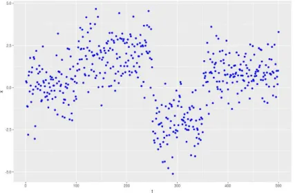
The epidemic changepoint model assumes that data follows a typical distribution for most of the time but deviates from it during certain segments, the start and end point of which for epidemic changes. To formalise this, consider a univariate time seriesx1, ..., xn. It is said to obey the epidemic changepoint model if there exists a setFigure 2.3.2: An example time series with K = 2 epidemic changes in mean. The first collective anomaly occurs between s1 = 100 and e1 = 150, and the second once occurs between s2 = 350 and e2 = 381.
of windows τ ={(s1, e1), ...,(sK, eK)}, where 0 ≤s1 < e1 ≤s2 < ...≤ sK < eK ≤n, such that xt∼ M1 s1 < t≤e1, .. . MK sK < t≤eK M0 otherwise 1≤t≤n.
Here, Mk denotes the model obeyed by the data during thekth epidemic change. In between these epidemic changes it follows the null model M0. An example of such a timeseries can be found in Figure 2.3.2. As in the classical changepoint case, setting
Mk =N(µk, σ2) gives rise to the change in mean problem with Gaussian noise. For simplicity, we will focus on this special case for the remainder of this section, pointing
to generalisations where appropriate.
Inferring at most one Single Change
The setting in which At Most One Change (AMOC) is present has received a sig-nificant amount of attention. This is because methodology detecting AMOC can naturally be extended to detect multiple changes, as we will show in Section 2.3.2. The problem of detecting a single epidemic change in mean can be formulated as the following hypothesis test (Yao, 1993): Consider data x1, ...., xn, where xi N(µi, σ2) and test the null hypothesis of a stationary mean.
H0 :µ1 =...=µn,
against the alternative hypothesis that some segment (s, e) has a different mean
H1 :∃s, e : 0≤s < e≤n, µ1 =...=µs=µe+1 =...=µn6=µs+1 =...=µe. This hypothesis testing framework can be extended to other types of epidemic changes, such as epidemic changes in variance, slope, mean and variance, etc.
The presence and location of epidemic changes are then typically inferred by using a likelihood ratio statistic (see, for example, Aston et al. (2012) and Yao (1993)). This likelihood ratio statistic is computed for all candidate start and end points. The pair of points for which this statistics is the largest is then declared a collective anomaly if the statistic exceeds a pre-defined thresholdλ. Otherwise, the alternative hypothesis is rejected. The thresholdλis typically increased with the number of observations to account for multiple testing. (Yao, 1988)
Inferring Multiple Changes
Arguably the most commonly used method for the detection of multiple epidemic changes is circular binary segmentation (CBS) introduced by Olshen et al. (2004). Like Binary Segmentation for classical changepoints, CBS is capable of extending any AMOC test statistic to multiple epidemic changes by repeatedly applying the AMOC procedure to the parts of the data currently deemed typical. The algorithms can be summarised as follows:
1. Apply the AMOC procedure to the data x1,...,xn and obtain candidate start and end points s and e.
2. If the statistic does not exceed the threshold λ stop. Otherwise consider (s, e) to be an epidemic changepoint
3. Repeat the above procedure on the sequencesx1,...,xs and xe+1,...,xn
The computational cost of CBS isO(n2), when the whole data is searched. A faster approximation was proposed by Venkatraman and Olshen (2007). Another approach at speeding up CBS consists of imposing a maximum lengthm for epidemic changes, which reduces the computational cost toO(mn).
On the choice of λ
The threshold λ is typically chosen in such a way that it controls the overall number of false positives at an acceptable level. SinceO(n2) possible start and end points are investigated, this problem is closely linked to multiple testing. When trying to detect
epidemic changes in mean against a 0-background for example, as is the case in the CNV data, the log-likelihood ratio statistic for a segment s, e simplifies to
T(s, e) = (e−s) 1 e−s e X t=s+1 xt !2 ,
assuming Gaussian noise. Yao (1988) showed that
P max 0≤s<e≤nT(s, e)≤(2 +)σ 2log(n) →1, as n→ ∞
under the null hypothesis for all >0. Here σ is the standard deviation of the noise. Consequently, settingλ= (2 +)σ2log(n) asymptotically controls the number of false positives.
2.3.3
Epidemic Changepoint Models for Multivariate Data
Many time series are multivariate and epidemic changes can manifest themselves across multiple components. One commonly considered model for multivariate epi-demic changes is the subset multivariate model, which assumes that components be-have independently of each other, but that their anomalous time periods are linked. An example where this model is applicable can be found in the CNV data. Indeed, when no copy number variation is present, the data is independent across individuals. However, copy number variations can be shared by multiple subjects meaning that collective anomalies are likely to affect a subset of individuals at similar locations on the genome.
As with univariate epidemic changepoint detection, we can extend any AMOC pro-cedure to multiple epidemic changes by circular binary segmentation. Consequently,
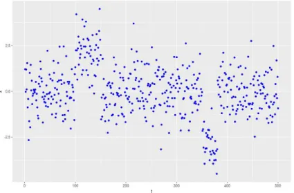
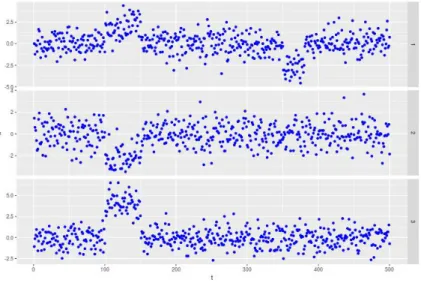
Figure 2.3.3: An example time series withK = 2 epidemic changes in mean. The first collective anomaly occurs betweens1 = 100 and e1 = 150 and affects all components, i.e. J1 ={1,2,3}. The second once occurs betweens2 = 350 and e2 = 381 and affects only the first component, i.e.J2 ={1}.
we will only review AMOC procedures in this section. In order to do so, we will begin by formalising the subset multivariate epidemic changepoint model before reviewing some theoretical results regarding sparse changes affecting few components strongly and dense changes which weakly affect a large number of components. This will be followed by a discussion of inference approaches.
Subset Multivariate Epidemic Changepoint Model
Consider multivariate data x1, ...,xn ∈ Rp. This data is said to contain a subset multivariate epidemic changepoint if there exists a subsetJ⊂ {1, ..., p}which exhibits a-typical behaviour during a time window (s, e). Formally we test the hypothesis
H0 :x (i) t ∼ M
(i)
which states that all n observations from the ith component follows the null model
M(0i) for 1≤i≤p against the alternative hypothesis
H1 :∃0≤s < e≤n,J ⊂ {1, ..., p}: x (i) t ∼ M(1i) s < t≤e, i∈J M(0i) otherwises
that an anomalous segment exists during which the ith component obeys a model
M(1i) which is different from its typical model M(0i) for i∈J.
Detectability Boundaries
Subset multivariate epidemic changes can be easier or harder to detect depending on how strong the changes are and how many components are affected. The literature (Jeng et al., 2012; Cai et al., 2011a) typically distinguishes between sparse changes, in which only a few components are affected by strong anomalies and dense changes which affect a large set of components, but potentially by very little. This has been formalised for the changes in mean and variance by Cai et al. (2011a) who for a segments, e considered testing the null hypothesis of uncontaminated data
H0 :x (i)
t ∼N(0,1) 1 ≤i≤p, s < t≤e against the alternative hypothesis of contaminated data
H0 :x (i)
t ∼(1−vi)N(0,1) +viN(µ,1 +σ2) 1≤i≤p, s < t≤e
where the independent random variables vi ∼ Ber(p−ξ) for 0 ≤ ξ < 1 determine whether the ith component exhibits anomalous behaviour or not. The parameter ξ
then determines whether the regime is sparse (ξ > 12) or dense (ξ≤ 1
of the change in mean (e−s)|µ| can the be parametrised as (e−s)|µ|= p 2rplog(p) ξ > 12 p−rp ξ ≤ 1 2, , rp >0
depending on whether the anomalous segment is dense or sparse. It is then called detectable if the exists a test whose type 1 and type 2 error both converge to 0 as
p→ ∞. Jeng et al. (2012) showed that the detectability boundary for the case ξ > 12
was ρ−= min ξ− 1 2−σ 2,1−(1 +σ2)p (1−ξ) 2
and that such a test exists if rp > ρ− and does not exist if rp < ρ−. Similarly the authors showed that the detectability boundary for the case ξ≤ 1
2 was ρ−< 1 2 −ξ σ= 0 ∞ σ >0
and that a consistent test exists if rp < ρ− and does not exist if rp > ρ−. Boundary cases for the related problem of distinguishing between mixtures were treated in Cai et al. (2011a).
In particular these results mean that even the smallest changes in variance make any dense change detectable. Another point of interest is that the signal strength of a dense change can go to 0 as p goes to infinity without the change becoming undetectable.
Inference Approaches
A variety of methods has been proposed to detect epidemic changes, dense and/or sparse, in multivariate data. For example, Zhang et al. (2010) computes a likelihood ratio statistic for each of the p components individually and the sums these, hence obtaining a tests statistic for a given start and end point. This test statistic is good for dense changes but lacks power for detecting sparse ones. Conversely, the approach suggested by Jeng et al. (2010) consists of considering the largest test statistic only, an approach suitable only for sparse changes.
Approaches capable of detecting both sparse and dense epidemic changes have also been proposed. These approaches typically test each component individually thus obtainingpdifferent p-values, which they then process to obtain a global significance value. The methods of both Zhang et al. (2010) and Jeng et al. (2010) fall into this framework thought they have good power only against certain types of epidemic changes. One example an approach suitable for both sparse and dense changes is proportion adaptive segment selection (PASS), introduced by Jeng et al. (2012), uses higher criticism (Donoho and Jin, 2004). Higher criticism builds on the fact that all p-values q1, ..., qp are i.i.d. U(0,1) distributed under the null hypothesis. Consequently, the ordered p-valuesq(1) ≤...≤q(p) are all Beta distributed under the null hypothesis. This motivates the higher criticism statistic which is defined as:
HCp∗ = max 1≤i≤p(HCp,i), HCp,i = √ p i p −q(i) p q(i)(1−q(i)) .
(2012) showed that a threshold value of
(1 +) log(nm) + 2 log(log(p))
p
2 log(log(p)) ,
for some >0 asymptotically controls the number of false positives, as well as having power against all detectable sparse and most detectable dense alternatives. However, this asymptotic result is based on the asymptotic (and slow) convergence of the higher order statistic to a non-degenerate random variable (Shorack and Wellner, 2009). To improve finite sample performance, and reduce the number of false positives in particular, the authors suggest to consider maxα0≤i≤p(HCp,i) instead, where α0 ∈ N
is greater than 1. However, this is only advisable if no collective anomalies of interest affects fewer than α0 components.
Other methods for combining the individualp-values have also been proposed. For example, the adaptive Fisher procedure Song et al. (2016), which exploits the fact that the differences between the logarithms of the ordered p-values is exponentially distributed under the null. Entirely different principal component analysis based approaches have also been proposed (Aston et al., 2012).
Collective And Point Anomalies
3.1
Introduction
Anomaly detection is an area of considerable importance for many time series applica-tions, such as fault detection or fraud prevention, and has been subject to increasing attention in recent years. See Chandola et al. (2009) and Pimentel et al. (2014) for comprehensive reviews of the area. As Chandola et al. (2009) highlight, anomalies can fall into one of three categories: global anomalies, contextual anomalies, or col-lective anomalies. Global anomalies and contextual anomalies are defined as single observations which are outliers with regards to the complete dataset and their local context respectively. Conversely, collective anomalies are defined as sequences of ob-servations which are not anomalous when considered individually, but together form an anomalous pattern.
A number of different approaches can be taken to detect point (i.e. contextual and/or global) anomalies. These are observations that do not conform with the
tern of the data. Hence, the problem of detecting point anomalies can be reformulated as inferring the general pattern of the data in a manner that is robust to anomalies. The field of robust statistics offers a wide range of methods aimed at this problem. For instance, Rousseeuw and Yohai (1984) proposed S-estimators to robustly esti-mate the mean and variance. These estimators were later extended to a multivariate setting by Rousseeuw (1985). A wide variety of robust time series models also exist. For example, Muler et al. (2009) proposed a robust ARMA model, Muler and Yohai (2002) a robust ARCH model, and Muler and Yohai (2008) a robust GARCH model. A robust non-parametric method, which decomposes time series into trend, seasonal component, and residual was proposed by Cleveland et al. (1990).
The machine learning community has also provided a rich corpus of work for the detection of point anomalies. Commonly used methods include nearest neighbour based approaches, such as the local outlier factor (Breunig et al., 2000), and infor-mation theoretical methods such as the one introduced by Guha et al. (2016). It is beyond the scope of this chapter to review them all. Instead we refer to excellent reviews that can be found in Chandola et al. (2009) and Pimentel et al. (2014). Lavin and Ahmad (2015), Talagala et al. (2019), Ahmad et al. (2017), and references therein provide examples of more recent developments in the area.
One common drawback of several point anomaly approaches is their limited ability to detect anomalous segments, or collective anomalies. Such features are of signifi-cance in many applications. One example is the analysis of brain imaging data, where periods in which the brain activity deviates from the pattern of the rest state have been associated with sudden shocks (Aston and Kirch, 2012). Another example is in
detecting regions of the genome with unusual copy number (Bardwell and Fearnhead, 2017; Siegmund et al., 2011; Zhang et al., 2010), with such copy number variation being associated with diseases such as cancer (Jeng et al., 2012).
The current statistical literature mostly uses hidden Markov models, smoothing based approaches or epidemic changepoint methods for the detection of collective anomalies. Hidden Markov models assume that a hidden state chain determines whether the data produced is anomalous or typical (Smyth, 1994). The underlying assumption that anomalous segments share one or multiple common behaviours is very attractive for some applications, such as brain imaging, where it can be assumed that there is a finite number of states, but can be a constraint in others. Hidden Markov models also suffer from the fact that they are not robust to global anomalies. Moreover, they tend to be slow to fit, which is an important disadvantage in many modern, big-data applications. This is in stark contrast with the typically very fast smoothing based approaches like the one proposed by Schwartzman et al. (2011). However, the smoothing step limits interpretability making the approach vulnerable to point anomalies and differentiating between point and collective anomalies nigh impossible. Furthermore, these methods achieve optimal power when the bandwidth of the smoothing kernel is of the same length-scale as the collective anomalies, meaning that they can struggle when anomalies are of very different lengths.
The epidemic changepoint model, first introduced by Levin and Kline (1985) as-sumes that there is a typical behaviour, from which the data deviates during col-lective anomalies. Epidemic changepoints can therefore be viewed as two classical (non-epidemic) changepoints: one away from and one back to the typical
distribu-tion. Thus, a simple approach to detecting collective anomalies would be to use one of the many methods for changepoint detection (e.g. Fearnhead and Rigaill, 2019a, Fryzlewicz, 2014, James et al., 2016, Killick et al., 2012, Ma and Yau, 2016, and ref-erences therein). However this does not exploit the fact that the behaviour of the segment before the start and after the end of an anomalous segment is the same. This reduces its statistical power, as can be seen in Section 3.5, which is a disadvantage, especially when faced with a weak signal.
The main corpus of work addressing the problem of detecting epidemic changes has been driven by the analysis of neuroimaging and genome data. An early ap-plication of epidemic changepoints to neuroimaging data can be found in Robinson et al. (2010), who use a hidden Markov model to detect epidemic changes in mean. This was later extended by Aston and Kirch (2012). Both methods are vulnerable to point anomalies, a shortcoming in some applications like the ones we consider in this chapter. Another limitation is that both approaches assume the presence of at most one change. Conversely, motivated by challenges arising in Genomics, a range of methods, both univariate and multivariate, have been proposed to detect epidemic changes in mean, mainly by considering sum of squares type test statistics (see Jeng et al., 2012; Siegmund et al., 2011; Cai et al., 2012), sometimes in combination with hidden states. They are therefore vulnerable to global anomalies. A more general Bayesian hidden state method for the detection of anomalous segments was proposed by Bardwell and Fearnhead (2017).
This article makes two main contributions. The first is the introduction of an esti-mation procedure that allows for the identification ofCollectiveAndPointAnomalies
(CAPA). Secondly, we establish finite sample consistency results not only for CAPA, but also for a commonly used penalised cost based method (Killick et al., 2012) aimed at detecting changes in mean and variance. This setting presents significant additional technical challenge compared to the change in mean setting, to which most existing theoretical results apply. Since the first version of this work appeared on arXiv, a sim-ilar algorithm has been independently proposed by Zhao and Yau (2019). However, the work of Zhao and Yau (2019) does not contain any consistency results and does not address the challenge of fitting point anomalies when using a data distribution with multiple parameters (e.g. changes in mean and variance).
The article is organised as follows: We begin by introducing a parametric model with epidemic changes in Section 3.2. This provides a general framework for collective anomalies, the location of which we infer by minimising a penalised cost. In Section 3.3, we introduce an algorithm which minimises an approximation to the penalised cost based on a robust estimate of the parameter of the typical distribution. This approximation can be minimised by a dynamic programme.
Section 3.4 presents a number of theoretical results. Specifically, we introduce a proof of consistency for the detection of joint classical changes in mean and variance using a penalised cost approach, which is of independent interest. We then prove that CAPA consistently estimates the number and location of collective anomalies, despite the simplicity of the approach used for the estimation of the parameters of the typical distribution. Section 3.5 concludes with a discussion of penalties. We then compare CAPA to other methods in a simulation study in Section 3.5 and show that it outperforms them, especially in the presence of point anomalies.
The chapter is concluded by applying CAPA to two real datasets in Section 3.6. The first dataset is lightcurve data gathered by the Kepler space telescope. There we show that CAPA can be used to detect Kepler 1132-b, an exoplanet which orbits the star Kepler 1132 (Morton et al., 2016). The second dataset is a machine temperature dataset obtained on an expensive industrial machine. There we show that CAPA can be used to detect both critical failures as well as early warning signs, highlighting the algorithms usefulness for predictive maintenance. The proofs of the theoretical results are all given in the appendix. CAPA has been implemented in the R package anomaly(Fisch et al., 2020) which is available from CRAN.
3.2
A Modelling Framework for Collective
Anoma-lies
We assume that the data follow a parametric model where collective anomalies are epidemic changes in the model parameters. Whilst, in practice, it is unlikely that the distribution of the data in an anomalous segment will belong to the same family of distributions as the distribution of the typical data, it can nevertheless be expected that a set of parameters different from the typical distribution’s will offer a better fit. We say that datax1, ...,xn follow a parametric epidemic changepoint model if xt has
probability density function f(xt, θ(t)) and θ(t) = θ1 s1 < t≤e1, .. . θK sK < t≤eK, θ0 otherwise,
where θ0 is the, usually unknown, parameter of the typical distribution, from which the model deviates during theK anomalous segments (s1, e1),...,(sK, eK) by adopting behaviours characterised by the parametersθ1, ..., θK all different fromθ0. We assume these windows do not overlap, i.e.e1 ≤s2, ..., eK−1 ≤sK. Note that fitting an epidemic changepoint requires only one new set of parameters forθ, since the typical parameter is shared across the non-anomalous segments. This compares favourably with the two additional sets of parameters forθ introduced when an epidemic changepoint is fitted using two classical changepoints. We can therefore expect to gain statistical power, which is confirmed by the empirical results in Section 3.5.
It is possible to infer the number and location of epidemic changes by choosing ˜K, (˜s1,˜e1),...,(˜sK˜,e˜K˜), and ˜θ0, which minimise the penalised cost
X t /∈∪[˜si+1,˜ei] C(xt,θ˜0) + ˆ K X j=1 min ˜ θj ˜ ej X t=˜sj+1 C(xt,θ˜j) +β , (3.2.1)
subject toei−si ≥ˆl, where ˆl is the minimum segment length for an appropriate cost function C(x, θ) and a suitable penalty β. For example, C(x, θ) could be defined as the negative log-likelihood of x under the parametric model using parameter θ. A common choice for the penalty β would then be Clog(n) (Yao, 1988; Killick et al., 2012; Fryzlewicz, 2014), where the constantC depends on the model considered.
Using the formulation in (3.2.1), we can infer the location of joint epidemic changes in mean and variance by minimising the penalised cost related to the negative log-likelihood of Gaussian data. In this case θ = (µ, σ2) contains both the mean and variance and we estimate K, s1, ..., sK, and e1, ..., eK by minimising
X t /∈∪[˜si+1,˜ei] " log(σ20) + x t−µ0 σ0 2# + ˜ K X j=1 " (˜ej−s˜j) log P˜ej t=˜sj+1(xt−x¯(˜sj+1):˜ej) 2 (˜ej−s˜j) ! + 1 ! +β # , (3.2.2) subject to ˜ei −s˜i ≥ 2, i.e. a minimum segment length of 2, to account for the fact that θ is two dimensional.
It is well known that many changepoint detection methods struggle in the presence of point anomalies in the data and tend to fit two changepoints around each of them (Fearnhead and Rigaill, 2019a). An approach based on minimising the above cost function is not intrinsically immune to this phenomenon either. However, given that point outliers can naturally be viewed as single observations with a larger variance, we can incorporate them in the model as epidemic changes, in variance only, of length one. We therefore choose ˜K, (˜s1,˜e1),...,(˜sK˜,e˜K˜), µ0, σ0, as well as the set of point anomalies O ⊂ {1, ..., n}, which minimise the modified penalised cost
X t /∈∪[˜si+1,e˜i]∪O " log(σ20) + xt−µ0 σ0 2# +X t∈O log (xt−µ0)2+γσ02 + 1 +β0 + ˆ K X j=1 " (˜ej −˜sj) log Pe˜j t=˜sj+1(xt−x¯(˜sj+1):˜ej) 2 (˜ej−s˜j) ! + 1 ! +β # , (3.2.3) whereβ0 is a penalty smaller than β. This modification ensures that it is now cheaper to fit an outlier as an epidemic changepoint in variance only than as a full epidemic change. The constant,γ >0 ensures that the argument of the logarithm will be larger than 0. We recommend settingγ to the level of precision of the observations, subject
to requiringγ >exp(−β0) which ensures that no inliers are fitted as point anomalies, as shown by Proposition 3 in Section 3.4.
This modification has the added benefit that it allows the algorithm to distinguish between point and collective anomalies. This property is important for a range of applications in which collective and point anomalies have different interpretations (see Section 3.6.1 for an example).
3.3
Estimation of Collective and Point Anomalies
We now turn to consider the problem of minimising the penalised cost we introduced in the previous section. Unlike in the classical changepoint problem considered by Jackson et al. (2005), the penalised cost given by equation (3.2.1) can not be minimised using a dynamic programme, since the parameterθ0is shared across multiple segments and typically unknown. We therefore use robust statistics to obtain an estimate, ˆθ0, forθ0. Such robust estimates can be obtained for a variety of models (Hampel et al., 1986; Jureˇckov´a and Picek, 2005). For example, the median, M-estimators, or the clipped mean can be used to robustly estimate the mean. The inter quartile range, the median absolute deviation, or the clipped standard deviation can be use to estimate the variance. Robust regression is available to estimate the parameters of AR models.
Having obtained ˆθ0, we then minimise
X t /∈∪[ˆsi+1,ˆei] C(xt,θˆ0) + ˆ K X j=1 min ˆ θj ˆ ej X t=ˆsj+1 C(xt,θˆj) +β , (3.3.1)
as an approximation to (3.2.1). Since it can be expected that most data belongs to the typical distribution, ˆθ0 should be close to θ0. One might therefore expect that
using this estimate will have little impact on the performance of the method, which we also show theoretically for joint changes in mean and variance in Section 3.4.2.
The approximation to the penalised cost in (3.3.1) can be minimised exactly by solving the dynamic programme
C(m) = min " C(m−1) +C(xm,θˆ0), min 0≤k≤m−ˆl C(k) + minθˆ m X t=k+1 C(xt,θˆ) ! +β ! # , (3.3.2) whereC(m) is the cost of the most efficient partition of the first m observations and
C(0) = 0. For example, solving the dynamic programme
C(m) = min " C(m−1) + log(ˆσ20) + xm−µˆ0 ˆ σ0 2 , min 0≤k≤m−2 C(k) + (m−k) " log 1 m−k m X t=k+1 xt−x¯(k+1):m 2 ! + 1 # +β ! # ,
minimises the approximate penalised cost for joint epidemic changes in mean and variance defined in equation (3.2.2), thus inferring the number and location of collec-tive anomalies. Similarly, we can minimise the approximation to its point anomaly robust analogue in equation (3.2.3) by solving the dynamic programme
C(m) = min " C(m−1) + log(ˆσ02) + xm−µˆ0 ˆ σ0 2 , min 0≤k≤m−2 C(k) + (m−k) " log 1 m−k m X t=k+1 xt−x¯(k+1):m 2 ! + 1 # +β ! , C(m−1) + 1 + log γσˆ02+ (xm−µˆ0)2 +β0 # ,
thus also inferring the number and location of point anomalies, with a negligible increase in computational cost. We call this algorithm CAPA. Pseudocode for the full CAPA algorithm is given by Algorithm 1 in the appendix.
Solving the full dynamic program is at least O(n2). This is because it requires n
steps over a solution space 0≤k ≤m−l, which is of sizeO(n) on average. However, we can reduce the size of the solution space by borrowing ideas on pruning from Killick et al. (2012), provided the loss function is such that adding a free changepoint will not increase the cost – a property which holds for many commonly used cost functions such as the negative log-likelihood. Indeed, the following proposition holds:
Proposition 1. Let the cost function C(·,·) be such that
min θ c X t=a C(xt, θ) ! ≥min θ b−1 X t=a C(xt, θ) ! + min θ c X t=b C(xt, θ) !
holds for all a, b, and csuch that a+ ˆl ≤b < c−ˆl. Then, if
C(k) + min θ m X t=k C(xt, θ) ! ≥C(m) (3.3.3)
holds for somek < m−ˆl, we can exclude that k from the solution space for all future steps m0 ≥m+ ˆl of the dynamic programme.
Thus we can keep track of the set of time indices that we need to minimise over in the dynamic programme. For each of these, we check, at each time step, if condi-tion 3.3.3 holds, and, if it does, we remove the index from the set. See steps 15-22 of Algorithm 2 in the appendix for more detail. This can significantly reduce the computational cost. In practice, we found that it was close to O(n) for the detection of joint epidemic changes in mean and variance when the number of true epidemic changes increased linearly with the number of observations. Note that the time after which a k can be discarded in the minimisation step also depends on the minimum segment length, something not considered by Killick et al. (2012).
3.4
Theory for Joint Changes in Mean and
Vari-ance
We now introduce some theoretical results for CAPA. In particular, we establish the consistency of CAPA at detecting collective anomalies and demonstrate that it can be viewed as a corollary of the consistency of a statistical procedure, such as optimal partitioning from Jackson et al. (2005) minimising a penalised cost function to detect classical (i.e. non-epidemic) changepoints. Consequently, we will begin by proving the consistency of a penalised cost method for the detection of changes in mean and variance in Section 3.4.1. To the best of our knowledge, no such result exists in the literature, which makes this proof of independent interest. We then proceed to proving the consistency of CAPA at detecting collective anomalies in Section 3.4.2. Like other cost function based approaches, CAPA is significantly affected by the choice of penalties. We therefore conclude this section by discussing suitable choices for this important hyper parameter in Section 3.4.3. The proofs of all theorems and propositions stated in this section can be found in the appendix.
3.4.1
Consistency of Classical Changepoint Detection
Consider the sequence x1, ..., xn ∈ Rn which is normally distributed with K ∈ N
changepoints. The sequence therefore satisfies xt = µ(t) +σ(t)ηt for ηt i.i.d.
where (µ(t), σ(t)2) = (µ1, σ12) t0+ 1≤t≤t1, .. . (µK+1, σK2+1) tK+ 1≤t ≤tK+1. (3.4.1)
Here 0 =t0 ≤...≤tK+1 =n denote the start of the series, the K changepoints, and the end of the series. We assume that the mean and/or variance changes at these changepoints, i.e. that (µk, σk2) = (6 µk+1, σ2k+1). These changes in mean and variance can be of varying strength. To quantify this, we define the signal strength4σ,k of the change in variance at the kth changepoint to be
42 σ,k = r σ k σk+1 − r σk+1 σk 2 = σk σk+1 +σk+1 σk −2. We note that 42
σ,k is equal to 0 if, and only if, σk+1 =σk. We also define the signal strength4µ,k of change in mean at the kth changepoint to be
4µ,k =
|µk−µk+1|
√
σkσk+1
.
Note that these two quantities can be combined into a global measure of signal strength 4k = log 1 + 1 24 2 σ,k+ 1 44 2 µ,k
for the kth change (see Lemma 7 in the appendix material for details).
We now define the penalised cost ˜C(xi:j, τ0, α) of data xi:j under partition τ0 =
{i−1,ˆt01, ...,ˆt0ˆ K0, j} to be ˜ C(xi:j, τ0, α) = ˆ K0 X k=0 ˜ C(x(ˆt k+1):ˆtk+1) + ˆK 0 αlog(n)1+δ,
for δ, α > 0. Here αlog(n)1+δ corresponds to the commonly used strengthened SIC-type penalty (Fryzlewicz, 2014; Li et al., 2016) for introducing an additional change-point. The cost of a segmentxa:b is set to be
˜ C(xa:b) = ˜C(xa:b,{a−1, b}) = (b−a+ 1) log Pb a(xt−x¯a:b) 2 b−a+ 1 ! + 1 ! ,
which is the same as the segment cost used to infer the location of epidemic changes in mean and variance. Since this leaves two parameters to fit, we impose a minimum segment length of two for all partitions.
We also introduce the following assumption which ensures that the changepoints are sufficiently spaced apart to allow for their detection:
Assumption 1. There exists some δ >˜ 0 such that for 1≤k ≤K+ 1
tk−tk−1 ≥
log(n)1+δ+˜δ
min(4k,42k,4k−1,42k−1)
,
where 40 =4K+1 =∞ for convenience of notation.
Here the fact that min(4k,42k,4k−1,42k−1) is used instead of min(42k,42k−1) as in the change in mean setting is due to the fact that we have moved from a sub-Gaussian to a sub-exponential setting.
Then, the following consistency result holds:
Theorem 1. Assume that observations x1, ..., xn follow the distribution specified in
Equation 3.4.1 and that Assumption 1 holds. LetKˆ andˆt1, ...,tˆKˆ be the number and
lo-cations of changepoints inferred by minimising the penalised cost functionC˜(x1:n, τ, α).