Signomial and Polynomial Optimization via Relative
Entropy and Partial Dualization
Riley Murray†, Venkat Chandrasekaran†,‡, and Adam Wierman† ∗
†
Department of Computing and Mathematical Sciences ‡ Department of Electrical Engineering
California Institute of Technology Pasadena, CA 91125
July 23, 2019
Abstract
We describe a generalization of the Sums-of-AM/GM Exponential (SAGE) relaxation methodology for obtaining bounds on constrained signomial and polynomial optimization problems. Our approach leverages the fact that rela-tive entropy based SAGE certificates conveniently and transparently blend with convex duality, in a manner that Sums-of-Squares certificates do not. This more general approach not only retains key properties of ordinary SAGE relaxations (e.g. sparsity preservation), but also inspires a novel perspective-based method of solution recovery. We illustrate the utility of our methodology with a range of examples from the global optimization literature, along with a publicly avail-able software package.
Keywords: global optimization, exponential cone programs, SAGE certificates, SOS certificates, signomial programming.
∗Email: [email protected], [email protected], [email protected]
Acknowledgements: R.M. was supported in part by an NSF Graduate Research Fellowship and by NSF grant CCF-1350590, NSF grant CCF-1637598, and AFOSR grant FA9550-16-1-0210. V.C. was supported in part by NSF grants CCF-1350590 and CCF-1637598, AFOSR grant FA9550-16-1-0210, and a Sloan Research Fellowship. A.W. was supported in part by NSF grant CCF-1637598.
1
Introduction
A signomial is a function of the form x7→Pm
i=1ciexp(αi·x) for real scalarsci and row vectors αi in R1×n. Signomial optimization (often called signomial
program-ming) concerns the minimization of a signomial, subject to signomial inequality and equality constraints. Signomial programming is a computationally challenging prob-lem with applications in chemical engineering [3], aeronautics [29], circuit design [15], and communications network optimization [20]. Signomials are sometimes thought of as generalizations of polynomials over the positive orthant; by a change of vari-ablesyi = expxi one arrives at “geometric form” signomialsy7→Pmi=1ciQnj=1y
αij
j . Despite this aesthetic similarity between polynomials and geometric-form signomi-als, we must bear in mind that signomials and polynomials have many significant differences. Where polynomials can be generated by a countably infinite basis, sig-nomials require an uncountably infinite basis. Where polysig-nomials are closed under composition, signomials are not. Where polynomials and exponential-form signo-mials are defined on all of Rn – geometric-form signomials are only defined on the
positive orthant.
For many years these abstract differences between signomials and polynomials have coincided with algorithmic disparities. Contemporary methods for signomial programming use some combination of local linearization, penalty functions, se-quential geometric programming, and branch-and-bound [11, 12, 14, 16, 18, 23, 24] – ideas which precede the advent of modern convex optimization. By contrast, the field of polynomial optimization has been substantially influenced by semidefinite programming, specifically through Sums-of-Squares (SOS) certificates of polyno-mial nonnegativity [5, 8, 10]. In recent work, Chandrasekaran and Shah proposed the Sums-of-AM/GM Exponential or SAGE certificates of signomial nonnegativity, which provided a new convex relaxation framework for signomial programs akin to SOS methods for polynomial optimization. [26]. Where SOS certificates make use of semidefinite programming, SAGE certificates use the convex relative entropy function. The authors of the present article further demonstrated that a natural modification to SAGE certificates leads to a tractable relative entropy representable sufficient condition for global polynomial nonnegativity [30].
This article is concerned with how proof systems for function nonnegativity can be used in the service of constrained optimization. The basic idea here is simple: for a function f, a set X, and a real number γ, we have inf{f(x) : x ∈ X} ≥ γ if and only if f −γ is nonnegative over X. The trouble is that to leverage this fact, we require ways to extend certificates for global nonnegativity (such as SOS or SAGE certificates) to prove nonnegativity over X ( Rn. For the polynomial
case one usually performs this extension by appealing to representation theorems from real algebraic geometry. In the absence of such representation theorems, one typically relies on a dual problem obtained from the minimax inequality.
The primary contribution of this article is to show how SAGE certificates – by virtue of their roots in convex duality – provide a simple and powerful alternative method for describing functions which are nonnegative over proper subsets of Rn.
Our method can be used both independently from and in conjunction with the min-imax inequality. The space of possibilities with our method is large, and it is far from obvious as to which variations of this methodology are most useful for given problem structures. To facilitate research in this regard, we provide a user-friendly software package which implements all functionality described in this article. We provide detailed worked examples in several places alongside conceptual develop-ment. A dedicated section on computational experiments is provided, and several avenues of possible future research are outlined in a discussion section.
1.1 Article outline and our contributions
This article makes both mathematical and methodological contributions to signomial and polynomial optimization. Section 2 speaks to key questions which help place our work in a broader context. These questions include (1) What are the sources of error in nonnegativity-based relaxations of constrained optimization problems, and how are they usually mitigated? (2) How exactly are the original SAGE cones formulated? (3) How can we understand partial dualization in the context of existing nonnegativity and moment relaxations?
Once these questions are answered, we introduce the concept of conditional SAGE certificates for signomial nonnegativity (Section 3). We prove a representa-tion result for the cone of these nonnegativity certificates (Theorem 6), and develop a solution recovery algorithm by investigating the dual cone (Algorithm 1). Sec-tion 3.4 describes two “hierarchies” of SAGE-based convex relaxaSec-tions for signomial programs: one which uses the minimax inequality, and one which is minimax-free. The authors know of no analog to the minimax-free hierarchy in the polynomial op-timization literature, and believe the underlying idea of the minimax-free hierarchy is of independent theoretical interest.
Section 4 extends the idea of conditional SAGE certificates to polynomials. We discuss basic properties of the conditional SAGE polynomial cones before proving representation results (Theorems 9 and 10) which provide the basis for tractable relaxations of constrained polynomial optimization problems. Section 4.2 provides simple descriptions for dual conditional SAGE polynomial cones, and develops an efficient solution recovery algorithm based on these descriptions (Algorithm 2). Sec-tion 4.4 proposes reference hierarchies for polynomial optimizaSec-tion with SAGE cer-tificates. Our minimax-free hierarchy has an interesting structure which reflects a link between SAGE signomials and SAGE polynomials, by way of the “signomial representatives” from [30].
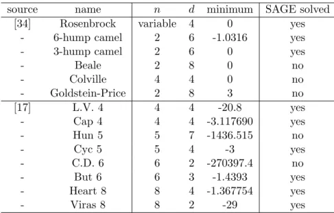
Section 5 reports the effectiveness of our methodology on fifty-one problems appearing in the literature (sourced from [1, 2, 17, 23, 24, 28, 31, 34]), as well as randomly generated problems. A central component of our experiments is a desire to facilitate research both into theory underlying conditional SAGE relaxations, and the practice of using these relaxations in engineering design optimization. Towards this end, we provide the “sageopt” Python package.1 Sageopt is a documented,
tested, and convenient platform for constructing and solving SAGE relaxations, as well as analyzing the results thereof. We used sageopt for all experiments in this article.
1.2 Notation and preliminary definitions
Vectors and matrices always appear in boldface. The ith entry of a vectorv is vi, and the vector formed by deleting theith entry of v isv\i. A matrix A is built by stacking rowsai ∈R1×n, and A\i is the submatrix formed by deleting the ith row of A. All logarithms in this article are base-e. Elementary functions from R toR
are extended first to vectors in an elementwise fashion, and subsequently to sets in a pointwise fashion. For a convex cone K⊂Rr, the dual cone is K†=. {y : y|x≥ 0 for allx inRr}. For A, B ⊂Rn, A⊂ B and A (B denote non-strict and strict
inclusion respectively. The operator “cl” computes set-closure with respect to the standard topology.
For an m×nmatrix α and a vector c in Rm, we write f = Sig(α,c) to mean
thatf takes values f(x) =Pm
i=1ciexp(αi·x). When α is a matrix of nonnegative
integers, we write f = Poly(α,c) to mean that c is the coefficient vector of f with respect to the monomial basis x7→ xαi =. Qn
j=1x
αij
j . Given a matrix α and a set X⊂Rn, one has the nonnegativity cones
CNNS(α, X)=. {c : Sig(α,c)(x)≥0 for allxinX}
and
CNNP(α, X)=. {c : Poly(α,c)(x)≥0 for allx inX}.
We write CNNS(α) and CNNP(α) in reference to the above cones when X = Rn.
Except in special cases onα, it is computationally intractable to check membership in eitherCNNS(α) orCNNP(α) [4]. The inner-approximations of nonnegativity cones
developed in this article make use of the relative entropy function; this is the convex function “D” with domainRm+ ×Rm+ taking values
D(u,v) = m
X
i=1
uilog(ui/vi).
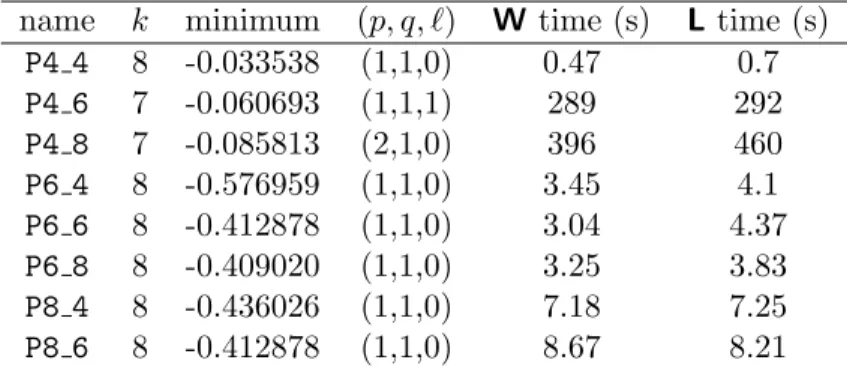
This article includes computational experiments with SAGE certificates and states solver runtimes for many of these examples. All of these examples rely on the MOSEK solver [32]. We use two different machines to provide a sense of when it may be practical to solve a SAGE relaxation with given computational resources. MachineWis an HP Z820 workstation, with two 8-core 2.6GHz Intel Xeon E5-2670 processors and 256GB 1600MHz DDR3 RAM. MachineL is a 2013 MacBook Pro, with a dual-core 2.4GHz Intel Core i5 processor and 8GB 1600MHz DDR3 RAM.
2
Background
In this article we study constrained nonconvex optimization problems of the form (f, g, φ)?X = inf{f(x) :xinX ⊂Rn, g(x)≥0, φ(x) =0} (1) wheref is a function fromRntoR,g mapsRn toRk1, and φmaps RntoRk2. Our
primary goal is to produce lower bounds (f, g, φ)lbX ≤(f, g, φ)?X. In the event that (f, g, φ)lbX = (f, g, φ)?X, we are also interested in recovering optimal solutions to (1). For ease of exposition, this section focuses on problems of the form (1) with only inequality constraints– i.e. the problem of bounding
(f, g)?X = inf{f(x) :xinX⊂Rn, g(x)≥0}. (1.1) In Section 2.1 we review the Lagrange dual relaxation of the above problem, both in minimax form and as a nonnegativity problem. Section 2.2 provides the minimum background on SAGE and SOS nonnegativity certificates needed develop the con-tributions of this article. In Section 2.3 we review standard techniques for strength-ening nonnegativity-based relaxations of problems such as (1.1); this includes the use of redundant constraints, nonconstant Lagrange multipliers, and strengthening nonnegativity certificates via modulation. Section 2.4 concludes with discussion on partial dualization. Until Section 2.4, the set X appearing in Problem 1.1 shall be the whole ofRn.
2.1 Dual problems in nonconvex optimization
The simplest way to lower bound (f, g)?Rn is via the Lagrange dual. For each
co-ordinate function gi of g, we introduce a dual variable λi ≥ 0 and consider the Lagrangian L(x,λ) =f(x)−λ|g(x). The Lagrange dual problem is to compute
(f, g)LRn = sup
λ≥0
inf
x∈RnL(x,λ).
By the minimax inequality, we can be certain that (f, g)L
Rn ≤(f, g)
?
Rn.
There are many situations when the Lagrange dual problem is intractable. For signomial and polynomial optimization, one usually needs to compute yet another lower bound (f, g)d
Rn ≤ (f, g)
L
Rn. Contemporary approaches for computing such
bounds begin by introducing a parameterized function ψ(γ,λ) which takes values ψ(γ,λ)(x) =L(x,λ)−γ. One reformulates the dual problem as
(f, g)LRn = sup{γ : λ≥0, γ inR, ψ(γ,λ)(x)≥0 for allxinRn},
and the constraint that “ψ(γ,λ) defines a nonnegative function” is then tightened to “ψ(γ,λ) satisfies a particular sufficient condition for nonnegativity.” The expecta-tion is that the sufficient condiexpecta-tion can be expressed by tractable convex constraints on variables γ and λ. For example, SOS certificates for polynomial nonnegativity can be expressed via linear matrix inequalities, and SAGE certificates for signomial and polynomial nonnegativity can be expressed with the relative entropy function.
2.2 SAGE and SOS nonnegativity certificates
In the development of the SAGE inner approximation forCNNS(α), Chandrasekaran
and Shah considered the structure where the coefficient vector ccontained at most one negative entry ck; if such a function was globally nonnegative, they called it an
AM/GM Exponential, or anAGE function [26]. One thus defines thekth AGE cone
CAGE(α, k) ={c:c\k ≥0 and cbelongs to CNNS(α)}.
A key contribution of [26] was the use of convex duality to derive an efficient descrip-tion of the AGE cones. The outcome of this derivadescrip-tion is that a vectorcbelongs to
CAGE(α, k) iffc\k≥0 and
some ν inRm+−1 has [α\i−1αi]|ν =0 and D(ν,c\k)−ν|1≤ck. (2) The system of constraints given by (2) is crucially jointly convex in c and the auxiliary variable ν. The set defined by thesum of all AGE cones
CSAGE(α)=. (
c: there existc(k) inCAGE(α, k) satisfying c=
m X k=1 c(k) ) (3)
is therefore efficiently representable.
The SAGE cone as defined above applies to signomials, but a similar construction exists for certifying global nonnegativity of polynomials [30]. Formally, we say that f = Poly(α,c) is an AGE polynomial if it is nonnegative over Rn, and if f(x)
contains at most one term cixαi that is not a monomial square. In conic form this writes as
CPOLYAGE (α, k) ={c: Poly(α,c)(x)≥0 for all xinRn, and
c\k≥0, ci = 0 for all i6=k withαi 6∈2N1×n}, (4)
and such AGE cones naturally give rise to
CPOLYSAGE(α)=. m
X
k=1
CPOLYAGE (α, k)⊂CNNP(α). (5)
The SAGE polynomial cone can also be described by an appropriate reduction to the SAGE signomial cone. For a nonnegativem×ninteger matrixαand a vector
c inRm, we define the set ofsignomial representative coefficient vectors as
SR(α,c) ={cˆ: ˆci =ci whenever αi is in 2N1×n, and
ˆ
ci ≤ −|ci|wheneverαi is not in 2N1×n}.
The name “signomial representative” derives from the fact that if ˆc belongs to SR(α,c), then nonnegativity of the signomial Sig(α,ˆc) would evidently imply non-negativity of the polynomial Poly(α,c) (see Section 5.1 of [30]). The set SR(α,c)
is useful because a constraint of the form “ˆc belongs to SR(α,c)” is jointly convex in cˆand c. Lemma 19 of [30] proves that the SAGE polynomial cone defined by Equation 5 is equivalently given by
CPOLYSAGE(α) ={c : SR(α,c)∩CSAGE(α) is nonempty }.
The generalization of SAGE polynomials considered in this article benefits from both the Sum-of-AGE-function and signomial-representative viewpoints of ordinary SAGE polynomials.
Lastly we consider Sums-of-Squares (SOS) polynomials. A polynomialf is said to be SOS if it can be written in the form f = Pm
i=1fi2 for appropriate polyno-mials fi. In the context of polynomial optimization, one usually parameterizes the SOS cone by a number of variables n and a maximum degree 2d; this cone can be represented as
SOS(n,2d) ={p : p(x) =Lnd(x)|MLnd(x), M 0}
whereLn
d :Rn→R(
n+d
d ) is the map from a vector xto the vector of all monomials
of degree at-most-d evaluated at x. The connection between SOS-representability and semidefinite programming was first observed by Shor [5], and was subsequently developed by Parrilo [8] and Lasserre [10].
2.3 Strengthening dual bounds in nonnegativity relaxations
A common method for strengthening dual problems is to introduce redundant con-straints to the primal problem, particularly by taking products of existing constraint functions. As an example of this principle in action, consider the toy polynomial optimization problem
inf{ −x2 : −1≤x≤1}=−1. One may verify that (f, g)L
R=−∞, but by adding the single redundant constraint
(1−x)(1 +x)≥0, we can certify a dual bound −1≤(f, g)?
R.
A more subtle method is to reconsider what is meant by “dual variables.” For the Lagrange dual problem we use scalars λi ≥ 0, however it would be just as valid to have λi be a function, provided that it was nonnegative over Rn. Such a
method is well-suited to our nonnegativity-based relaxations of the dual problem. The following toy signomial program illustrates the utility of this approach
inf{−exp(2x) : 1≤exp(x)≤2}=−4.
Again the Lagrange dual problem returns a bound of−∞, but by considering λi of the form λi(x) =ηiexp(x) withηi ≥0, the resulting dual bound is−4≤(f, g)?
R.
Our third method for strengthening dual bounds only becomes relevant when working with strict inner-approximations of nonnegativity cones. For two functions w, f with w positive definite, it is clear that f is nonnegative if and only if the product w·f is nonnegative. The method of modulation is to choose a generic
positive-definite functionwso that iff fails a particular test for nonnegativity (say, being SOS, or being SAGE), there is still a chance that the productw·f passes a test for nonnegativity. Indeed, modulation is a crucial tool for computing successive bounds for unconstrained problems
fR?n = inf. {f(x) :xinRn}= sup{γ:f(x)−γ ≥0 for allx inRn}.
Suppose for example thatf is a signomial over exponentsα; then forw= Sig(α,1) we can compute a non-decreasing sequence of lower bounds
f(`)
Rn = sup{γ :γ inR, w
`(f −γ) is SAGE} ≤f?
Rn.
Under appropriate conditions onα(c.f. [26]), these lower bounds converge tof?
Rnas
`goes to infinity. From an implementation perspective, the constraint that “ψ(γ)=. w`(f −γ) is SAGE” is tractable because the coefficient vector of ψ(γ) is an affine function of γ.
Modulation can similarly be applied to constrained optimization. Suppose that
L(x,λ) is the Lagrangian for Problem 1.1, and refer to the functionx7→ L(x,λ) as
L(λ). Then rather than requiring that “L(λ)−γ is SAGE”, one could require that “ψ(γ,λ)=. w`(L(λ)−γ) is SAGE.” This would increase the size of the feasible set for variables γ and λ, and remain tractable due to the affine dependence ofψ(γ,λ) on γ and λ. Such modulation leads to a non-decreasing sequence of bounds which converge to (f, g)L
Rn under suitable conditions. 2.4 Partial dualization
Apartial dual problem is what results when the set “X” in Problem 1.1 is a proper subset of Rn. In this case the natural generalization of the Lagrange dual is
(f, g)dX = sup. {γ : λ≥0, γ inR, L(x,λ)−γ ≥0 for all xinX}. (6)
The technique of partial dualization refers to the deliberate choice to restrict the Lagrangian to X ={x: gi(x) ≥0 for all iinI} for some I ⊂ [k], even when the constraints {gi}i∈I are of a functional form that is permitted in the Lagrangian.
Note that in the extreme case with X = {x : g(x) ≥ 0}, we are certain to have (f,0)dX = (f, g)?
Rn – in this way, partial dualization provides a mechanism to
com-pletely eliminate duality gaps.
Before getting into how SAGE certificates integrate with partial dualization, it is worth considering a simple example which combines partial dualization and nonnegativity certificates. Suppose we want to minimize a univariate polynomialf over an interval [a, b], subject to a single polynomial equality constraintg(x) = 0. In this case we could form a LagrangianL(x, µ) =f(x)−µg(x) withµ∈R, and find the largest constantγ so thatL(x, µ)−γ was nonnegative overx∈[a, b]. A well-known result in real algebraic geometry is that a degree-d polynomial “p” is nonnegative over an interval [a, b] if and only if pcan be written as p(x) =s(x)2+h[a,b](x)t(x)2,
where h[a,b](x) = (b−x)(x−a), and s, t are polynomials of degree at most d and
d−1 respectively [9]. Therefore the partial dual problem
(f, g)d[a,b]= sup{γ : γ, µ∈R, f(x)−µg(x)−γ ≥0 for all x in [a, b]}
can be framed as an SOS relaxation
(f, g)d[a,b]= sup{γ :f−µg−γ =s+h[a,b]t
s∈SOS(1,2d), t∈SOS(1,2(d−1))}.
Our last key concept is how partial dualization manifests in the dual of the dual. To develop this idea, considerf = Poly(α,c) withα1=0, along with a setX⊂Rn.
The problem of computing f? X
.
= infx∈Xf(x) has the following convex formulation fX? = sup{γ : c−γ(1,0, . . . ,0) ∈ CNNP(α, X)}.
Of course, the above problem is intractable unless α and X satisfy very special conditions. In spite of the possible intractability, we can still compute the dual problem by applying standard rules of conic duality. The result of this process is
fX? = inf{c|v : v∈CNNP(α, X)†, v1 = 1}
where CNNP(α, X)† is the dual cone to CNNP(α, X). This second problem is what
we mean by “the dual of the dual.” It appears prominently in the literature on polynomial optimization, where it is usually referred to as a moment relaxation
[10]. The term “moment relaxation” derives from the fact thatCNNP(α,Rn)† is the
smallest closed convex cone containing the vectors
(Rn)α=. {(xα1, . . . ,xαm) : x∈Rn},
and by thinking of a convex hull as computing expectationsEx∼F[(xα1, . . . ,xαm)], where F is a probability measure over Rn. One can similarly understand the dual
of a nonnegativty-based partial-dual problem in terms of probability and moment relaxations. When X as a proper subset of Rn, the convex hull of Xα can be
framed as the set of all vector-valued expectationsEx∼F[(xα1, . . . ,xαm)], whereF is a probability measure over X. In this way, the “dual” of partial dualization can be understood in terms ofconditional moments.
3
Conditional SAGE certificates for signomials
In this section we show how SAGE certificates for signomial nonnegativity can fully leverage partial dualization, in the sense that any efficiently representable convex set X gives rise to a parameterized and efficiently representable “X-SAGE” non-negativity cone. The efficient representation of theX-SAGE cones (which we often call “conditional SAGE cones”) leads to a practical, principled approach for solving and approximating a range of nonconvex signomial optimization problems. In this regard the most common sets X are of the form {x : g(x) ≤ 1} for signomials gi with all nonnegative coefficients. An algorithm for solution recovery, and two worked examples are provided.
3.1 The conditional SAGE signomial cones
Definition 1 (Conditional AGE signomial cones). For a matrix α in Rm×n, a subset X of Rn, and an indexk in [m], the kth AGE cone with respect to α, X is
CAGE(α, k, X) ={c∈Rm : c\k≥0 and Sig(α,c)(x)≥0 for all x in X}. Definition 2 (X-SAGE signomials). If the vector c belongs to
CSAGE(α, X)=.
m
X
k=1
CAGE(α, k, X)
thenf = Sig(α,c) is an X-SAGE signomial.
Conditional SAGE cones are order-reversing with respect to the second argu-ment. That is, if X2 ⊂ X1 ⊂ Rn, then CSAGE(α, X1) ⊂ CSAGE(α, X2) for all α
in Rm×n. Note that CSAGE(α, X) is defined for arbitrary X ⊂ Rn, including
non-convex sets, and non-convex sets which admit no efficient description. Moreover, as a mathematical object, CSAGE(α, X) does not depend on the representation ofX.
In practice we need conditions on X in order to optimize over CSAGE(α, X).
But before we get to those, it is worth mentioning some abstract results concerning optimization. Forf = Sig(α,c) withα1=0, define
fXSAGE= sup. {γ : γ inR, c−γ(1,0, . . . ,0) inCSAGE(α, X)}
so that fXSAGE≤fX? = inf. {f(x) :xinX}.
Theorem 3. If c≥0, then f = Sig(α,c) has fXSAGE =fX? for allX ⊂Rn.
Proof. Let e1 = (1,0, . . . ,0). The signomial ˜f = Sig(α,c−fX?e1) is nonnegative
overX, and its coefficient vectorc−fX?e1contains at most one negative entry. This
implies that ˜f is X-AGE, and henceX-SAGE.
Theorem 4. If X is bounded, then fXSAGE>−∞ for every signomial f.
Proof. If X is empty then the result follows by verifying that CSAGE(α, X) = Rm.
Consider the case when X is nonempty. In this situation it suffices to prove the result for all f of the form f(x) = cexp(a ·x) where c 6= 0 and a belongs to
R1×n. Fixing suchc, a, the boundedness ofX implies the existence ofL6= 0 with
˜
f(x) =cexp(a|x) +Lnonnegative overxinXand cL <0. Since ˜f is nonnegative overXand contains exactly one negative coefficient, we have thatfSAGE
X ≥ −L.
Corollary 5 (See [30]). Let X ⊂Rn be arbitrary. If c is a vector in C
SAGE(α, X)
with nonempty N ={i:ci <0}, then there exist vectors {c(i)}i∈N satisfying c(i)∈CAGE(α, i, X) c=
X
i∈N
Proof. This is simply the statement of Theorem 2 from [30], which was proven for ordinary SAGE cones, i.e. withX =Rn. The entire proof of that theorem (including
Lemmas 6 and 7 of [30]) extends to conditional SAGE cones simply by replacing references to “CAGE(α, i)” and “CSAGE(α)” with “CAGE(α, i, X)” and “CSAGE(α, X)”
respectively.
In order to reliably optimize over CSAGE(α, X), we need X to be a tractable
convex set. This is essentially the only requirement on X, as is shown by the following theorem.
Theorem 6. For a matrixα inRm×n, an indexiin[m], and a convex setX⊂Rn with support function σX(λ)= sup. x∈Xλ|x, we have
CAGE(α, i, X) ={c:ν in Rm−1,c in Rm,λ in Rn satisfy
σX(λ) +D(ν,c\i)−ν|1≤ci,
[α\i−1αi]|ν +λ=0, and c\i≥0}.
Proof. Let δX denote the indicator function of X, taking values
δX(x) =
(
0 ifx belongs toX
+∞ if otherwise .
A vector c withc\i≥0belongs to CAGE(α, i, X) if and only if
p?= inf{δX(x) +P`
i=1˜ciexpti : x∈Rn, t∈R`, t=W x} ≥ −L (7)
for`=m−1,W = [α\i−1αi]∈R`×n,˜c=c\i∈R`, andL=ci.
The dual to the above optimization problem is easily calculated by applying Fenchel duality (c.f. [13]); the result of this process is
d?= sup{−σX(λ)−D(ν,˜c) +ν|1 : λ∈Rn,ν ∈Rm−1, W|ν +λ=0}. (8)
When X is nonempty, one may verify that the hypothesis of Corollary 3.3.11 of [13] (concerning strong duality) hold for the primal-dual pair (7)-(8). In particular, p? ≥ −L holds if and only if −d? ≤ L, and the dual problem attains an optimal solution whenever finite. WhenX is empty, it is clear thatp? = +∞, and by taking both λand ν as zero vectors, we have d? = +∞. The result follows.
Theorem 6 is stated in terms of support functions for maximum generality. From an implementation perspective, it is useful to assume a representation of X. For example, if X ={x : Ax+b∈K} for a matrixA, a vector b, and a convex cone K, then weak duality ensures
An upper bound on the support function is all we need to construct an inner-approximation of a given AGE cone. For allX ={x : Ax+b∈K}, we have
{c:ν inRm−1,c inRm, and ηin K†
D(ν,c\i)−ν|1+η|b≤ci,
[α\i−1αi]|ν =A|η, and c\i≥0} ⊂CAGE(α, i, X).
If there exists an x0 so that Ax0+bbelongs to the relative interior ofK, then by
Slater’s condition the reverse inclusion in the preceding expression also holds.
3.2 Dual perspectives and solution recovery
Here we discuss how dual SAGE relaxations can be used to recover optimal and near-optimal solutions to signomial programs of the form (1). For concreteness, we state the simplest such relaxation here. Let f, {gi}ik=11 and {φi}ki=12 be signomials
over exponents α, with α1 =0. If c is the coefficient vector of f, and the rows of
G∈Rk1×m,Φ∈
Rk2×m specify coefficient vectors ofgi,φi respectively, then inf{c|v :v∈CSAGE(α, X)†, v1 = 1, Gv≥0, Φv=0} (9)
is a convex relaxation of Problem 1. It is readily verified that if v? is an optimal solution to (9) andv? = exp(αx) for some x inX, thenxis optimal for (1).
The prospect of inverting the moment-type vector v? to obtain a feasible point
x∈Xdrives our interest in understanding the dual coneCSAGE(α, X)†. By standard
rules in convex analysis, the dual SAGE cone is given by
CSAGE(α, X)†=∩i∈[m]CAGE(α, i, X)†.
An expression for the dual AGE cones can be recovered from Theorem 6. Using coX ={(x, t) : t >0, x/t∈X}to denote the cone overX, the usual conic-duality calculations yield
CAGE(α, i, X)†= cl{v:vilog(v/vi)≥[α−1αi]z
(z, vi)∈coX, v inR+m, and z inRn}. (10)
The auxiliary variables “z” appearing in the representation for the dual X-AGE cones are a powerful tool for solution recovery. Ifz,v satisfy the constraints in (10) withvi >0, thenx=. z/vi belongs toX. Additionally, if the inequality constraints involving the logarithm are binding and we meet the normalization condition vi = exp(αi·x), then we will have exp(αx) =v.
These observations form the core – but not the entirety – of our solution recovery algorithm. Depending on solver behavior and dimension-reduction techniques used to simplify a SAGE relaxation, it is possible thatv= exp(αx) for somexinX, and yet no dual AGE cone generated this value. Therefore it is also prudent to solve a constrained least-squares problem to findxinX withαx near logv.
Algorithm 1 signomial solution recovery from dual SAGE relaxations.
Input: Signomials f, {gi}ki=11 , and {φi}ki=12 over exponents α inRm×n. A vector v
inCSAGE(α, X)†. Infeasibility tolerances ineq, eq ≥0.
1: procedure SigSolutionRecovery(f, g, φ,α,v, ineq, eq)
2: solutions←[]
3: for j= 1, . . . ,length(v)do
4: Recover z inRn s.t. vjlog(v/vj)≥[α−1αj]z and (z, vj)∈coX.
5: x←z/vj.
6: solutions.append(x).
7: end for
8: if αx6= logv for all xin solutions then
9: Compute xlsin argmin{klogv−αxk : xinX}.
10: solutions.append(xls).
11: end if
12: solutions←[xin solutions if g(x)≥ −ineq and|φ(x)| ≤eq ].
13: solutions.sort(f,increasing).
14: return solutions.
15: end procedure
Assuming that Equation 10 is used to represent the dual AGE cones, the runtime of Algorithm 1 is dominated by Line 10. The runtime of Line 10, in turn, should be substantially smaller than the time required to computev ∈CSAGE(α)†which is
optimal for an appropriate SAGE relaxation.
Note how Algorithm 1 implicitly assumes that v is elementwise positive. For numerical reasons, this will be the case in practice. At a theoretical level, if v
contains some component vi = 0, then there is no x in Rn which could attain
vi = exp(αi ·x), and so solution recovery is not a well-posed problem in such situations. Note also how in the important (and possibly nontrivial) case with k1=k2 = 0, Algorithm 1 always returns at least one feasible solution.
In the authors experience it is useful to take solutions generated from Algorithm 1 and pass them to a local solver as initial conditions. This additional step is especially worthwhile when there is a gap between a SAGE bound and a problem’s true optimal value, or when solution recovery to the desired precision of ineq, eq
fails. The term “Algorithm 1L” henceforth refers to the use of Algorithm 1, followed by local-solver solution refinement. For the examples in this article, the authors use Powell’s COBYLA solver for the solution refinement [6].2
2
A FORTRAN implementation is accessible through SciPy’soptimize submodule. The argu-ments we pass to that FORTRAN implementation areRHOBEG=1,RHOEND= 10−7, andMAXFUN= 105.
3.3 A first worked example
The following problem has appeared in many articles concerning algorithms for signomial programming [11, 14, 16, 18, 23].
inf
x∈R3 f(x) .
= 0.5 exp(x1−x2)−expx1−5 exp(−x2) (Ex1)
s.t. g1(x)= 100. −exp(x2−x3)−expx2−0.05 exp(x1+x3)≥0
g2:4(x) = expx−(70,1,0.5)≥0
g5:7(x) = (150,30,21)−expx≥0
This problem (“Example 1”) is an excellent candidate for conditional SAGE re-laxations, because each of the seven constraints defines an efficiently representable convex set. Constraint functions g2:7 can be can be represented with six linear
in-equalities, and the constraint functiong1 can be represented with three exponential
cones and one linear inequality. As a separate matter, Example 1 is interesting be-cause the Lagrange dual problem performs poorly: regardless of how many products we take of existing constraint functions gi, the −5 exp(−x2) term in the objective
will cause Lagrangians f −P
IλIQj∈Igj to be unbounded below for all values of dual variablesλI ≥0.
Now we describe how SAGE relaxations fare for Example 1. We begin by setting X={x:g1:7(x)}; sinceXis bounded, Theorem 4 tells us thatfXSAGEis finite. The dual SAGE relaxation can be solved with MOSEK on Machine Lin 0.01 seconds, and provides us with a lower boundfXSAGE =−147.86≤fX?. By running Algorithm 1 on the dual solution, we recover
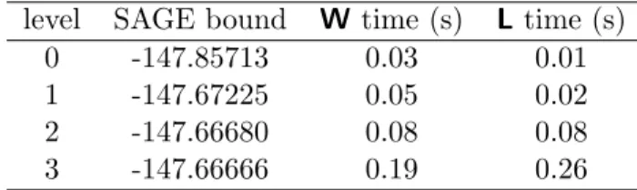
x? = (5.01063529, 3.40119660,−0.48450710) satisfying f(x?) =−147.66666. From this solution, we know that the bound obtained from the SAGE relaxation is within 0.13% relative error of the true optimal value. The ability to recover near-optimal solutions even in the presence of a gapfXSAGE< fX? can be attributed to how our solution recovery algorithm differs from traditional “moment” techniques. As it happens, the pointx? recovered from Algorithm 1 is actually an optimal solution to Example 1. In order to certify this fact, we need stronger SAGE relaxations. Table 1 shows the results of these relaxations, using the minimax-free hierarchy described in Section 3.4.
level SAGE bound W time (s) Ltime (s)
0 -147.85713 0.03 0.01
1 -147.67225 0.05 0.02
2 -147.66680 0.08 0.08
3 -147.66666 0.19 0.26
Table 1: SAGE bounds for Example 1, with solver runtime for MachinesW and L. A level-3 bound certifies the level-0 solution as optimal, within relative error 10−8.
3.4 Reference hierarchies for signomial programming
This section gives a particular set of choices regarding SAGE-based hierarchies for signomial programming. Because SAGE certificates are sparsity-preserving, one must be careful when describing relaxations which use nonconstant Lagrange mul-tipliers, or positive-definite modulators. In particular, when we say “f and gi are signomials over exponents α,” we mean that {x 7→exp(αj ·x)}mj=1 is the smallest
monomial basis spanning all linear combinations of f, gi, and the function that is identically equal to one.
First we describe a SAGE-based hierarchy that does not make use of the minimax inequality. This could be understood as a hierarchy for unconstrained optimization, but really applies whenever minimizing a signomial over a tractable convex set X ⊂ Rn. In the event that we cannot certify nonnegativity f −γ with γ = fX?,
we can use modulators as described in Section 2.3 to improve the largest SAGE-certifiable bound onf. Formally, for a signomialf over exponentsα, a nonnegative integer`, and a tractable convex set X, thelevel-`SAGE relaxation forfX? is
fX(`) = sup. {γ : Sig(α,1)`(f −γ) is X-SAGE}.
The special case with `= 0 was introduced earlier in this section as “fXSAGE.” Now we consider the case with functional constraints; letf,gi, andφi be signo-mials over exponentsα. SAGE relaxations for the problem of computing (f, g, φ)?X are indexed by three integer parameters: p,q, and`. Starting fromp≥0 andq≥1, define α[p] as the matrix of exponent vectors for Sig(α,1)p, and defineg[q] as the set of all products of at-most-q elements of g (similarly define φ[q]). The SAGE relaxation for (f, g, φ)?X at level (p, q, `) is then
(f, g, φ)(Xp,q,`)= sup γ s.t. sh, zh are signomials over exponentsα[p] (11)
L=. f−γ−P
h∈g[q]sh·h− P
h∈φ[q]zh·h
Sig(α,1)`L is anX-SAGE signomial sh areX-SAGE signomials.
The decision variables in (11) areγ ∈R, the coefficient vectors of{sh}h∈g[q], and the
coefficient vectors of{zh}h∈φ[q]. The most basic level of this hierarchy is (p, q, `) =
(0,1,0). This corresponds to using scalar Lagrange multipliers (sh≥0 andzh ∈R),
the original constraints (g[0] = g, φ[0] = φ), and modulating the Lagrangian by the signomial that is identically equal to 1. Note that when p > 0, the Lagrange multipliers sh are required to be nonnegative only over X, rather than over the whole ofRn.
Once an appropriate SAGE relaxation has been solved, there is the matter of attempting to recover a solution from the dual problem. Oftentimes a SAGE re-laxation produces a tight bound on (f, g, φ)?X, and yet no feasible solution can be recovered from Algorithm 1 with reasonable values of eq. Thus we also suggest
that one eliminate equality constraints through substitution of variables, when pos-sible. When it is not possible to eliminate all equality constraints, we recommend
allowing large violations of equality constraints in Algorithm 1 (e.g. eq= 1.0), and
passing the returned values as near-feasible points to a local solver in the manner of Algorithm 1L.3 This principle also extends to allowing large values of ineq prior
to solution-refinement, however the authors find that this is usually not necessary.
3.5 A second worked example
This section’s example can be found in the 1976 PhD thesis of James Yan [1], where it illustrates signomial programming in the service of structural engineering design. This problem is notable because it is nonconvex even when written in exponential form. Such signomial programs have received limited attention in the engineering design optimization community, largely due to a lack of reliable methods for solving them. We restate the problem here (as Example 2) in geometric form.4
inf A∈R3++ P∈R++ 104(A1+A2+A3) (Ex2) s.t. 104+ 0.01A−11A3−7.0711A−11 ≥0 104+ 0.00854A−11P−0.60385(A1−1+A−21)≥0 70.7107A−11−A1−1P−A−31P = 0 104 ≥104A1≥10−4 104 ≥104A2≥7.0711 104 ≥104A3≥10−4 104 ≥104P ≥10−4
Let X ⊂R4 be the feasible set cut out by the eight bound constraints in Example
2. With an X-SAGE relaxation where all constraints appear in the Lagrangian, we obtain (f, g, φ)(0X,1,0) = 14.1423 in 0.04 seconds of solver time. This bound is very close to the optimal value claimed by Yan [1]. However, Algorithm 1 only returns candidate solutions “x” with equality constraint violationsφ(x)≈70.
In an effort to improve our chances of solution recovery, we use the equality con-straint todefinethe valueP ←70.7107A3/(A3+A1). After clearing the denominator
(A3+A1) for inequality constraints involvingP, we obtain a signomial program (in
geometric-form) in only the variablesA1, A2, A3. We solve a level-(0,1,0) dual
con-ditional SAGE relaxation for this signomial program, and exponentiate the result of Algorithm 1 to recover
A= (7.0711000e−04, 7.0711000e−04, 1.00000000e−08), P = 70.7107A3 A1+A3
. This solution is feasible up to machine precision, and attains objective matching the 14.142300 SAGE bound. The entire process of solving the SAGE relaxation and recovering the optimal solution takes less than 0.05 seconds on MachineW.
3COBYLA is an excellent example of a solver which suppports infeasible starts. 4
The objective and inequality constraint functions are multiplied by 104 for numerical reasons; see equation environment (6.15) on page 106 of [1] for the original problem statement.
3.6 Remarks on “geometric-form” signomial programming
By now we have seen signomial programs in both exponential and geometric forms. The authors have hitherto preferred the exponential form, primarily because it al-lows us to build upon the substantial theories of convex analysis and convex opti-mization. However it is important to acknowledge that from an applications per-spective, it is far more common to express signomial programs in geometric form. Here we briefly present a geometric-form parameterization of conditional SAGE certificates for signomial nonnegativity – both in effort to appeal to those who are accustomed to working with geometric-form signomial programs, and as a prelude to our discussion on conditional SAGE polynomials.
Geometric form signomials f(x) = Pm
i=1cixαi are defined at points x inRn++,
and so it only makes sense to discuss conditional nonnegativity cones for signomials over setsX⊂Rn
++. Henceforth, define CGEOMNNS (α, X) ={c : Pm
i=1cixαi ≥0 for allx inX}
for matrices α in Rm×n and sets X contained in Rn++. By applying the change of
variables x7→expyand considering the subsequent change of domain X 7→logX, one may verify thatCGEOMNNS (α, X) =CNNS(α,logX). Thus forX⊂Rn++, one arrives
naturally at the definition
CGEOMSAGE (α, X)=. CSAGE(α,logX).
From here it should be easy to deduce various corollaries for CGEOMSAGE (α, X), by ap-pealing to results from Section 3.1. The most important such result is that one can efficiently optimize over CGEOMSAGE (α, X) whenever logX is a convex set for which the epigraph of the support function is efficiently representable.
4
Conditional SAGE certificates for polynomials
In the previous section we saw how conditional SAGE certificates for signomial nonnegativity are inextricably linked to convex duality. Here we show how the broader idea of conditional SAGE certificates can extend to polynomials. In this context it is not convexity ofXthat determines when anX-SAGE polynomial cone is tractable, but rather convexity of an appropriate logarithmic transform of X.
The organization of this section is similar to that of Section 3. Definitions, rep-resentations, and other basic theorems for the conditional SAGE polynomial cones are given in Section 4.1. Section 4.2 covers solution recovery from dual SAGE relaxations, and Section 4.3 provides a worked example with special focus on so-lution recovery. Section 4.4 describes reference hierarchies for optimization with conditional SAGE polynomial cones: one based on the minimax inequality, and one that is “minmax free.” Section 4.5 applies various manifestations of the minimax hierarchy to an example problem.
4.1 The conditional SAGE polynomial cones
We callf = Poly(α,c) anX-AGE polynomial if it is nonnegative overX, andf(x) contains at most one termcixαi which is negative for some xinX.
Definition 7(Conditional AGE polynomial cones). Forα in Nm×n, a subsetX of Rn, and an index iin [m], the ith AGE polynomial cone with respect to α, X is
CPOLYAGE (α, i, X) ={c: Poly(α,c)(x)≥0 for all xin X,
cj ≥0 if j6=iand xαj >0 for some xin X,
cj ≤0 if j6=iand xαj <0 for some xin X }. Let us work through some consequences of the definition. For starters, if xαj
takes on positive and negative values as x varies over X, then cj = 0 whenever
c ∈ CPOLYAGE (α, i, X) and i6= j. Note that xαj can only take on both positive and
negative values when αj does not belong to the even integer lattice. If X contains an open ball around the origin, thenxαj takes on both positive and negative values if and only if αj does not belong to the even integer lattice. Thus Definition 7 agrees with the definition of ordinary AGE polynomial cones, as proposed in [30] and as restated in Equation 4. Another important case is when X is a subset of the nonnegative orthant. This point is addressed in some detail later in this section; as a preliminary remark, we note that by considering the connection between polynomials and geometric-form signomials, one can easily see that if X ⊂ Rn++
then CPOLYAGE (α, i, X) = CAGE(α, i,logX). With these facts in mind, we define the
conditional SAGE polynomial cone in the natural way.
Definition 8 (X-SAGE polynomials). If the vector c belongs to
CPOLYSAGE(α, X)=. m
X
k=1
CPOLYAGE (α, k, X)
then we say that f = Poly(α,c) is anX-SAGE polynomial.
Many of our earlier theorems for signomials apply toX-SAGE polynomials with-out any special assumptions on X. For example, it is easy to show that Theorem 4 applies to conditional SAGE polynomials: if X is bounded, thenf = Poly(α,c) withα1=0has
fXSAGE= sup. {γ : γ in R, c−γ(1,0, . . . ,0) inCPOLYSAGE(α, X)}>−∞.
Corollary 5 likewise extends to polynomials. Other than substituting AGE signomial cones with AGE polynomial cones, the only difference is that N becomes N ={i: cixαi <0 for some xinX}.
Now we turn to representation of SAGE polynomial cones. By applying a simple continuity argument one can show that ifX= clX◦ ⊂Rn+– whereX◦is the interior
of X – then CPOLYSAGE(α, X) = CSAGE(α,logX◦). This claim is strengthened slightly
Theorem 9. Suppose X ⊂ Rn+ is representable as X = cl{x: 0 < x, H(x) ≤1}
for a continuous map H :Rn → Rr. Then for Y = {y : H(expy) ≤ 1}, we have
CPOLYSAGE(α, X) =CSAGE(α, Y).
The proof of Theorem 9 is straightforward, and hence omitted. A more so-phisticated result concerns whenX is not contained in any particular orthant, but nevertheless possesses a certain sign-symmetry.
Theorem 10. SupposeX ⊂Rnis representable as X= cl{x:0<|x|, H(|x|)≤1} for a continuous map H:Rn→Rr. Then for Y ={y:H(expy)≤1}, we have
CPOLYSAGE(α, X) ={c : SR(α,c)∩CSAGE(α, Y) is nonempty }. (12)
By combining Theorem 6 with Theorems 9 and 10, we know that there exist a range of sets X for which optimization over X-SAGE polynomials is tractable. There remains the potentially nontrivial task of formulating a problem so that one of these theorems provides an efficient representation of CPOLY
SAGE(α, X); important
examples of when this is possible include constraints such as
−a≤xj ≤a, kxkp≤a, |xαi| ≥a, and x2j =a wherea >0 is a fixed constant.
Proof of Theorem 10. Suppose thatcinCPOLYSAGE(α, X) admits the decompositionc=
Pm
i=1c(i), wherec(i) belongs to theith AGE polynomial cone with respect toα, X.
Define {˜c(i)}m
i=1 as follows
˜
c(ji)=
(
−|c(ji)| ifαi is not even, andj =i
c(ji) if otherwise .
By the invariance of X under reflection about hyperplanes {x : xj = 0}, and continuity of polynomials, we have that
0≤inf{Poly(α,c(i))(x) : x inX}= inf{Poly(α,˜c(i))(x) : xinX∩Rn+}
= inf{Sig(α,c˜(i))(y) : y inY}.
The signomials Sig(α,c˜(i)) are thus nonnegative overY ={y:H(expy)≤1}, and posses at most one negative coefficient. This implies that ˜c=. Pm
i=1c˜(i) belongs to CSAGE(α, Y). One may verify thatc˜also satisfies ˜c∈SR(α,c), and so we conclude
that the right-hand-side of Equation (12) containsCPOLYSAGE(α, X).
Now we address the reverse inclusion. Letcbe such that SR(α,c)∩CSAGE(α, Y)
is nonempty. One may verify that basic properties of CSAGE(α, Y) and SR(α,c)
ensure that if the intersection is nonempty, it contains an elementc˜satisfying|c|=
|˜c|. Henceforth fix c˜satisfying these conditions. Next we appeal to a relaxed form of Corollary 5. SettingN ={i: ˜ci≤0}, there exist vectorsc˜(i) satisfying
˜
c=P
Note how the definition of SR(α,c) ensures thatN ={i:αi is not even, orci ≤0}. Thus we define c(i) by
c(ji)=
(
(sgncj)|c˜j| ifαi is not even, andj =i ˜
c(ji) if otherwise
so thatc=P
i∈Nc(i), and eachc(i) has the necessary sign pattern for membership
in theith AGE cone with respect to α, X. Finally, note that
inf{Poly(α,c(i))(y) :xinX}= inf{Sig(α,c˜(i))(y) :y inY} ≥0. to complete the proof.
4.2 Solution recovery for sparse moment problems
This section concerns using dual SAGE relaxations to recover solutions to optimiza-tion problems of the form (1.1), where f and gi are polynomials over exponents α. If G a k×m matrix whose ith row is the coefficient vector of gi, α1 is the zero
vector, and cis the coefficient vector of f, then the simplest such relaxation is inf{c|v : v∈CPOLYSAGE(α, X)†, v1 = 1, Gv≥0}. (13)
Overall, our goal is to recover vectors xinX satisfying v = (xα1, . . . ,xαm), where v is an optimal solution to a relaxation such as the one above. We assume thatX is of a form where one of Theorems 9 or 10 provide a tractable representation of
CSAGE(α, X); this assumption allows us to leverage the following corollary.
Corollary 11. Fix Y ={y:H(expy)≤1} for a continuousH :Rn→Rr.
• If X= cl{x : 0<x, H(x)≤1}, then CPOLYSAGE(α, X)†=CSAGE(α, Y)†.
• If X= cl{x : 0<|x|, H(|x|)≤1}, then
CPOLYSAGE(α, X)†={v:there exists vˆ in CSAGE(α, Y)† with
|v| ≤vˆ, and vi= ˆvi whenαi ∈2N1×n}.
We make a running assumption that “Y” is convex.
Solution recovery for polynomial optimization is more difficult than for signomial optimization, because monomials possess both signs and magnitudes. We propose a two-phase approach for this problem, where different techniques are used to recover variable magnitudes and variable signs. The main ideas for each phase are described in Sections 4.2.1 and 4.2.2, while the formal algorithms are given in the appendix. The recovered signs and magnitudes are then combined in an elementary way, as given by the following algorithm.
Algorithm 2 solution recovery for dual SAGE polynomial relaxations.
Input: Polynomials f, {gi}ki=11 , and {φi}ki=12 over exponents α ∈ Nm×n. Vectors
v∈CPOLYSAGE(α, X)†and vˆ∈CSAGE(α, Y)†. Tolerances ineq, eq, 0 >0.
1: procedure PolySolutionRecovery(f, g, φ,α,v,ˆv, ineq, eq, 0)
2: M ←VariableMagnitudes(α, v, vˆ, 0). # Algorithm 3
3: S ← {1}
4: if X is not a subset ofRn+ then
5: S.union( VariableSigns(α, v) ) # Algorithm 4
6: end if
7: solutions←[].
8: for xmag inM and sinS do
9: x←xmags # denotes elementwise multiplication
10: if g(x)≥ −ineq and |φ(x)| ≤eq then
11: solutions.append(x) 12: end if 13: end for 14: solutions.sort(f, increasing). 15: return solutions. 16: end procedure
If v is optimal for Problem (13) and v = (xα1, . . . ,xαm) for an elementwise
nonzerox in X, then Algorithm 2 will return an optimal solution to Problem 1.1. As with Algorithm 1 in the signomial case, the authors find it useful to apply a simple local solver to the output of Algorithm 2 as a sort of solution refinement. We say “Algorithm 2L” in reference to such a method, with COBYLA as the local solver.
4.2.1 Recovering variable magnitudes
Givenv inCPOLYSAGE(α, X)†, we want to find x∈X satisfying (xα1, . . . ,xαm) =|v|.
Regardless of whether X is sign-symmetric or X ⊂ Rn
+, the variable v ∈ CPOLYSAGE(α, X) is associated with an auxiliary variable vˆ in CSAGE(α, Y), and the
variable vˆ is associated with additional auxiliary variables zi as part of the dual Y-AGE signomial cones. As we discussed in Section 3.2, the vectors yi = zi/ˆvi belong toY, and so the vectorsxi = expyi must belong toX. These vectorsxi are not only feasible with respect toX, but also satisfy
(xα1 i , . . . ,x
αm
i ) =vˆ (14)
under the binding-constraint and normalization conditions discussed in Section 3.2. Of course, if ˆv = |v|, then Equation (14) is precisely what we desire from our variable magnitudes. Since vˆ =|v| always holds at least for X ⊂ Rn
+, the vectors
When X is sign-symmetric, it is possible that vˆ does not equal |v|. This is particularly likely whenvis subject to additional linear constraints, such asGv≥0. Therefore when X is sign-symmetric it is worth considering variable magnitudes which supplement the ones described above. We propose that one picks a threshold 0>0, computes
y∈argmin{P
i:vi6=0(αi·y−log|vi|)
2 :y inY, (15)
αi·y≤log(0) for allvi = 0} and exponentiates x = expy. The role of 0 is to ensure that x = expy satisfies |x|αi ≤
0 whenevervi = 0. Extremely small values of0 (such as 10−100) would be
reasonable here.
A formal statement of our method for magnitude recovery (Algorithm 3) can be found in the appendix.
4.2.2 Recovering variable signs
For v in Rm, let α−1(v) denote the set of x∈ Rn satisfying v = (xα1, . . . ,xαm).
Henceforth, fix v and assume α−1(v) is nonempty. Here we describe how to find
vectors s in {+1,0,−1}n so that at least one x ∈ α−1(v) satisfies xi > 0 when
si = +1, xi = 0 when si = 0, and xi < 0 when si = −1. Once we describe this process, we relax the problem slightly so that si= +1 allows xi = 0.
First we address when si should equal zero. Let U = {i ∈ [m] : vi 6= 0}. Consider how if some x ∈ α−1(v) has xj = 0, then we must have αij = 0 for all i in U (else the equality xαi = v
i 6= 0 would fail). Thus when αij = 0 for all i in U, we set sj = 0 without loss of generality. Now let W = {j ∈ [n] : αij > 0 for some iinU}; these are indices for which sj is not yet decided. Consider the vector (v <0)∈ {0,1}nwith values (v<0)
i = 1 ifvi<0, and zero if otherwise. Let
α[U,:] be the submatrix ofα formed by rows{αi}i∈U, and similarly index (v <0). Finally, solve
α[U,:]z≡(v<0)[U] mod 2 and zj = 0 for all j in [n]\W (16) forz in{0,1}n. The remaining (sj)j
∈W aresj =−1 ifzj = 1 andsj = 1 otherwise. An individual solution to (16) can be computed efficiently by Gaussian elim-ination over the finite field F2. Standard techniques for finite-field linear algebra
also allow us to compute a basis for a null space of a matrix in mod 2 arithmetic (c.f. [19]), and so in principle one can readily recover all possible solutions to (16). In practice we must be careful, since the number of solutions to the linear system can easily be exponentially large inn (for example, whenα ≡0n×m mod 2). Our formal algorithm for sign recovery accounts for this fact, and employs an additional hueristic to handle the case when (16) is inconsistent. See the appendix for details.
4.3 A first worked example
This section’s example is to minimize a function appearing in the formulation of the cyclic n-roots problem. The general cyclic n-roots problem is a challenging
benchmark problem in computer algebra [7]. Our problem is to minimize f(x) =−64 7 X i=1 Y j∈[7]\{i} xj (Ex3)
over the box X = [−1/2,1/2]7. To the authors’ knowledge, this problem was first used as an optimization benchmark in the work by Ray and Nataraj, on computing the extrema of polynomials over boxes [17]. One may verify that fX? = −7, and that this objective value is attained at x(1) = 1/2 and x(2) = −1/2. Despite this problem’s simplicity, it requires nontrivial computational effort with SOS methods. The lowest relaxation order that allows Gloptipoly3 [21] to computefX? =−7 results in a semidefinite program that takes MOSEK 90 seconds to solve with MachineW. SAGE relaxations automatically exploit the structure in this problem. Since the seven functionsfi(x) = 1−64Q
j6=ixi areX-AGE and sum tof + 7, we have that
−7 ≤ fXSAGE ≤ fX?. To address the dual SAGE relaxation and solution recovery, we introduce the 8×7 matrix α, with final row α8 = 0, αii = 0 for i ≤ 7, and
αij = 1 for the remaining entries. Next we write X = {x : x2 ≤ 1/4}, and for Y ={y: exp(2y)≤1/4}numerically solve
fXSAGE= inf{−64·1|v1:7 : −vˆ≤v≤vˆ, vˆinCSAGE(α, Y)†, v8= ˆv8 = 1}=−7.
MOSEK solves this problem in 0.01 seconds with Machine W.
We recover candidate magnitudes by using the eight Y-AGE cones associated with the auxiliary variable ˆv ∈ CSAGE(α, Y)†. To machine precision, each of these
AGE cones yields the same candidate magnitude |x|= 1/2. The optimal moment vectorv=1/64 is elementwise positive, and so sign-pattern recovery is a matter of finding all solutions to the systemαz≡0 mod 2. There are exactly two solutions to this system: z(1)=0, andz(2) =1. The first of these gives rise to signss(1) =1, and the second of these results in s(2) =−1. By combining these candidate signs
with candidate magnitudes, we obtain candidate solutions{1/2,−1/2}; since these solutions are feasible and obtain objective values matching the SAGE bound, we conclude that both candidate solutions are minimizers off overX.
4.4 Reference hierarchies for POPs
IfX ⊂Rn
+, then one should use the same hierarchies described in Section 3.4, where
“Sig” is replaced by “Poly” and constraints that a function is “an X-SAGE signo-mial” are replaced by constraints that the function is “an X-SAGE polynomial.” This section focuses on the more complicated case when X is sign-symmetric.
Our reference hierarchy for functionally constrained polynomial optimization is similar to that used for signomial programming. Let f, {gi}k1
i=1, and {φi}
k2 i=1 be
polynomials over common exponents α ∈ Nm×n, and fix sign-symmetric X ⊂
Rn.
duplicate rows. The SAGE relaxation for (f, g, φ)?X at level (p, q, `) is then
(f, g, φ)(Xp,q,`)= sup γ s.t. sh, zh are polynomials over exponentsαˆ[p] (17)
L=. f−γ−P
h∈g[q]sh·h− P
h∈φ[q]zh·h
Poly(2α,1)`Lis an X-SAGE polynomial sh areX-SAGE polynomials.
As before, the decision variables areγ ∈R, and the coefficient vectors of{sh}h∈g[q], {zh}h∈φ[q]. The main difference between (17) and it’s signomial equivalent (11), is
that the Lagrange multipliers are slightly more complex in (17). This change was made to improve performance for problems where only a few rows of α belong to the nonnegative even integer lattice.
Our minimax-free reference hierarchy for polynomial optimization is meaning-fully different from the signomial case. We begin by assuming a representationX= cl{x : 0 <|x|, H(|x|) ≤1}, and subsequently defining Y ={y : H(expy) ≤1}. LetAandCbe operators on polynomials so thatf = Poly(A(f),C(f)) always holds, and let s be the vector in Rm with si = 1 when αi is even, and si = 0 otherwise. The SAGE relaxation for f?
X at level (p, q) is
fX(p,q)= sup γ (18)
s.t. ψ= Poly(. α,s)p(f−γ)
c∈SR(A(ψ),C(ψ))
[Sig(A(ψ),1)]qSig(A(ψ), c) is Y-SAGE over optimization variablesc and γ.
Formulation (18) uses two parameters out of desire to mitigate both sources of error in the SAGE polynomial cone: the error from replacing a polynomial by its signomial representative, and the error from replacing the signomial nonnegativity cone by the SAGE cone. As we show in Section 5.2, the signomial representative complexity parameter “q” can make the difference in our ability to solve problems when X=Rn.
4.5 A second worked example
The following problem appears in work on “Bounded Degree Sums-of-Squares” (BSOS) and “Sparse Bounded Degree Sums-of-Squares” (Sparse-BSOS) methods for polynomial optimization [28, 31]. The latter paper reports that BSOS and Sparse-BSOS compute (f, g)?
R6 = −0.41288 in 44.5 and 82.1 seconds respectively,
when using SDPT3-4.0 on a machine with a quad-core 2.6GHz Core i7 processor and 16GB RAM.
inf x∈R6 f(x)=. x61−x62+x63−x64+x65−x66+x1−x2 (Ex4) s.t.g1(x)= 2x. 16+ 3x22+ 2x1x2+ 2x36+ 3x24+ 2x3x4+ 2x56+ 3x26+ 2x5x6 ≥0 g2(x)= 2x. 21+ 5x22+ 3x1x2+ 2x23+ 5x24+ 3x3x4+ 2x25+ 5x26+ 3x5x6 ≥0 g3(x)= 3x. 21+ 2x22−4x1x2+ 3x23+ 2x24−4x3x4+ 3x25+ 2x26−4x5x6 ≥0 g4(x)=. x21+ 6x22−4x1x2+x23+ 6x24−4x3x4+x52+ 6x26−4x5x6≥0 g5(x)=. x21+ 4x62−3x1x2+x23+ 4x64−3x3x4+x52+ 4x66−3x5x6≥0 g6:10(x)= 1. −g1:5(x)≥0 g11:16(x) =x≥0
This problem (Example 4) is a good example for conditional SAGE polynomial relaxations, because it allows for several choices in partial dualization.
The simplest choice is to use no partial dualization at all– simply solve relaxations of the form (17) with X = Rn. Indeed, it is possible to solve Example 3 with
only these ordinary SAGE certificates, however the necessary level of the hierarchy (f, g)(1,1,0)
R6 =−0.41288 requires 101 seconds of solver time on Machine W.
A strictly preferable alternative is to apply partial dualization with X = R6+.
With this choice ofX it is natural to drop the first two and last six constraints from g(all of which will be trivially satisfied), and work with ˆg=g3:10. This allows us to
compute (f,g)ˆ (1X,1,0)=−0.41288 in 3.04 seconds of solver time on Machine W, and 4.4 seconds of solver time on Machine L. It is significant that the SAGE relaxation can be solved in this amount of time on MachineL, since it is an order of magnitude faster than BSOS solve time reported in [31].
The most aggressive choice for partial dualization isX ={x : x≥0, g6:7 ≥0}.
With this choice of X one has the option of using ˆg = (g3:5, g8:10), or ˆg =g3:10; in
the first case Machine W computes (f,ˆg)(1X,1,0) =−0.47121 in 3.3 seconds, and in the second case Machine W computes (f,g)ˆ (1X,1,0) = −0.41288 in 5.67 seconds. It is worth emphasizing that even though g6:7 were incorporated into X, the SAGE
bound with Lagrange multiplier complexityp= 1 improved by including g6:7 in the
Lagrangian.
5
Computational experiments
This section presents the results of some computational experiments with SAGE relaxations. Experiments with signomial programs consist of twenty-nine problems drawn from the literature, of which seventeen are solved to optimality (see Section 5.1). Examples for polynomial optimization include twenty-two problems from the literature (Section 5.2), as well as randomly generated problems (Section 5.3).
All experiments described here were run with the provided sageopt python package. Sageopt is an extension and refinement of the “sigpy” package intro-duced by the authors in the appendix of [30]. In the spirit of Gloptipoly3 [21],
sageopt includes its own basic rewriting system to cast a SAGE relaxation into conic forms acceptable by appropriate solvers. The rewriting system also provides mechanisms for computing constraint violations, analyzing low-level problem data, and constructing a set X (in an appropriate representation) from lists of constraint functions g and φ. Once problem data f,g, and φare defined, a SAGE relaxation can be constructed and solved in just two lines of code. Solution recovery simi-larly requires no more than two lines of code. Sageopt currently supports the conic solvers ECOS [22, 25] and MOSEK [32].
Unless otherwise stated, experiments were conducted on MachineW. All exper-iments were conducted with the MOSEK solver, using the default solver tolerances. We note that although Sections 3.4 and 4.4 only stated the SAGE relaxations in primal form, these experiments were conducted by symbolically constructing pri-mal and dual problems, and solving them separately from one another. In order to communicate the quality of these numeric solutions, we generally report “SAGE bounds” to the farthest decimal point where the primal and dual objectives agree.
5.1 Signomial programs from the literature
The examples in this section were drawn from the PhD thesis of James Yan [1], a popular benchmarking paper by Rijckaert and Martens [2], and the more contempo-rary works [23, 24]. The organization of this section is chronological with respect to these three sources. Many of the problems considered here can be found elsewhere in the literature, including work by Shen et al. [11, 14, 18], Wang and Liang [12] and Qu et al. [16].
SAGE recovers best-known solutions for all but six of the twenty nine problems considered here. For every one of these six problematic examples, numerical issues resulted in solver failures for level-(p, q, `) relaxations wheneverp >0; the results for these six problems should not be taken as definitive. For the twenty-three problems where SAGE recovered best-known solutions, there are two important trends we can observe. First, our solution recovery algorithms are more likely to succeed with a conditional SAGE relaxation than with an ordinary SAGE relaxation, even when the ordinary SAGE relaxation is tight. Second– the local solver refinement in Algorithm 1L can help tremendously not only in the presence of suboptimal strictly-feasible initial solutions (Example 8), but also in the presence of both large and small constraint violations (Examples 9 and 6 respectively). The initial condition from a SAGE relaxation in Algorithm 1L is important; the underlying COBYLA solver can and will return suboptimal solutions if initialized poorly.
5.1.1 Problems from the PhD thesis of James Yan
We attempted to solve nine example problems appearing James Yan’s 1976 PhD thesis Signomial programs with equality constraints : numerical solution and ap-plications [1]. This section reproduces two of the six problems which we solved to global optimality via SAGE certificates. Yan’s “Problem B” (page 88) and “Problem
C” (page 89) serve as our Examples 5 and 6 respectively.
inf
x∈R4
f(x)= 2. −exp(x1+x2+x3) (Ex5)
s.t. g1(x)= 4. −expx3−15 exp(x2+x3)−15 exp(x3+x4)≥0
g2:5(x)= (1,. 1,1,2)−expx≥0
g6:9(x)= exp. x−(1,1,1,1)/10≥0
φ1(x)= exp. x1+ 2 expx2+ 2 expx3−expx4 = 0
It is possible to quickly compute (f, g, φ)?
R4 = 1.925 with both conditional and
ordinary SAGE certificates, although conditional SAGE certificates exhibit better performance for solution recovery. Specifically, (f, g, φ)(1,1,0)
R4 = 1.92592592 can be
computed in 0.12 seconds, but no solution can be recovered from Algorithm 1 unless is set to an unacceptably large value of 0.1. Instead we set X ={x : g(x)≥0}, compute (f, g, φ)(1X,1,0) = 1.92592593 in 0.18 seconds, and by running Algorithm 1 recoverx? satisfying g(x?)>1E-11,|φ(x?)|<1E-8, and f(x?) = 1.92592593.
inf
y∈R3 ++
y10.6y2+y2y3−0.5+ 15.98y1+ 9.0824y22−60.72625y3 (Ex6) s.t.y2−2y3−y1y2−2−0.48≥0
y10.5y23−y10.25y3−y22−5.75≥0 (1000,1000,1000)≥y≥(0.1,0.1,0.1) y12+ 4y22+ 2y32−58 = 0
y1y2−1y23.5+y2y3−y22−16.55 = 0 SettingX ={x∈R3 : g(x)≥0}, we can compute (f, g
1:2, φ)(0X,1,0) =−320.722913 in 0.04 seconds. By running Algorithm 1 with ineq =1E-8 and eq =1E-6, we
recover x with objective f(x) = −320.722913 and that is feasible up to tolerance 8E-7. We then pass this solution to COBYLA with parameterRHOEND=1E-10, and subsequently recover recoverx? with the same objective, but constraint violation of only 5E-13.
The remaining problems which we solved to optimality were “Problem A” on page 60, “Problem A” on page 88, “Problem D” on page 89, and the problem in equation environment “(6.15)” on page 106. The last of these was introduced in Section 3.5 as “Example 2.” The problems which we did not solve to optimality were “Problem B” on page 61, the problem in equation environment “(6.29)” on page 113, and the problem in equation environment “(6.36)” on page 120. In each of these unsolved cases, we encountered solver-failures for level-(p, q, `) relaxations whenever p >0. Therefore the bounds computed for each of these problems were essentially limited to those of Lagrange dual problems, with modest partial dualization.
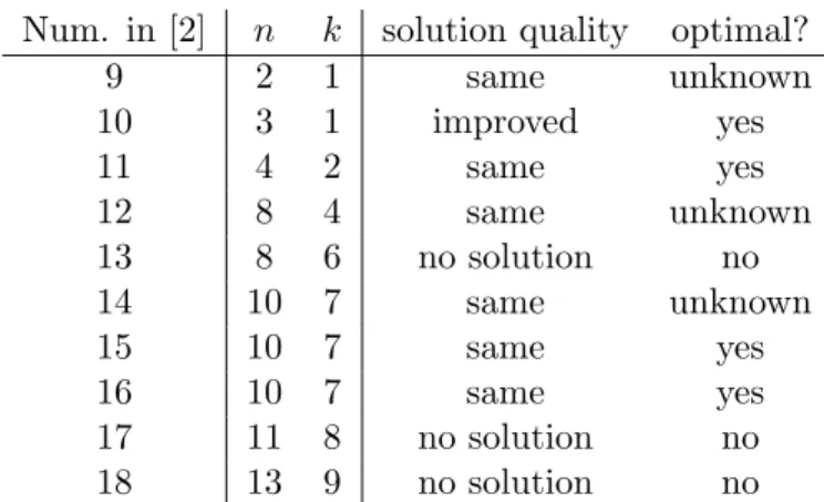
5.1.2 Problems from the benchmarking paper of Rijckaert and Martens We attempted to solve problems 9 through 18 of the popular signomial-geometric programming benchmark paper by Rijckaert and Martens [2]. Of these ten prob-lems, seven met with at least moderate success, in that SAGE relaxations produced meaningful lower bounds on a problem’s optimal value, and also facilitated recovery of best-known solutions to these problems. SAGE certificates allow us to certify global optimality for four of these seven problems. Problem statistics and a quali-tative summary of SAGE performance is given in Table 2.
We reproduce Rijckaert and Martens’ problems 10 and 15 as our Examples 7 and 8 respectively; both problems are written in exponential-form.
inf
x∈R3 f(x) .
= 0.5 exp(x1−x2)−expx1−5 exp(−x2) (Ex7)
s.t. g1(x)= 100. −exp(x2−x3)−expx1−0.05 exp(x1+x3)≥0
g2:4(x)= (100,. 100,100)−expx≥0
g5:7(x)= exp. x−(1,1,1)≥0
The bound constraints appearing in Example 7 are not included in [2], however f is unbounded below if we omit them. The solution proposed in [2] has expx = (88.310,7.454,1.311), and objective value f(x) =−83.06. The actual optimal solu-tion has value−83.25, and this can be certified by running Algorithm 1 on a dual solution for fX(3) = −83.2510, where X = {x : g(x) ≥ 0}. Solving the necessary SAGE relaxation takes 0.1 seconds on Machine W.
inf
x∈R10
f(x)= 0.05 exp. x1+ 0.05 expx2+ 0.05 expx3+ expx9 (Ex8)
s.t. g1(x)= 1 + 0.5 exp(x. 1+x4−x7)−exp(x10−x7)≥0 g2(x)= 1 + 0.5 exp(x. 2+x5−x8)−exp(x7−x8)≥0 g3(x)= 1 + 0.5 exp(x. 3+x6−x9)−exp(x8−x9)≥0 g4(x)= 1. −0.25 exp(−x10)−0.5 exp(x9−x10)≥0 g5(x)= 1. −0.79681 exp(x4−x7)≥0 g6(x)= 1. −0.79681 exp(x5−x8)≥0 g7(x)= 1. −0.79681 exp(x6−x9)≥0
A level (1,1,0) ordinary SAGE relaxation for Example 8 can be solved in 2.8 seconds on MachineW; this returns the bound (f, g)(1,1,0)
R10 = 0.2056534. When Algorithm 1
is run on the dual solution, it returns a point xsatisfying f(x)≈0.38 and g(x)≥
0.053. However by subsequently running Algorithm 1L, we obtain x? satisfying f(x?) = 0.20565341 and gi(x?) ≥ 1E-8 for all i in [k]. We thus conclude that the level-(1,1,0) SAGE relaxation was tight.