Nayha Mansoor
A Thesis Submitted for the Degree of PhD
at the
University of St Andrews
2020
Full metadata for this thesis is available in
St Andrews Research Repository
at:
http://research-repository.st-andrews.ac.uk/
Please use this identifier to cite or link to this thesis:
http://hdl.handle.net/10023/19506
This item is protected by original copyright
This item is licensed under a
Creative Commons License
Three Essays In Labour Economics
Nayha Mansoor
This thesis is submitted in partial fulfilment for the degree of
Doctor of Philosophy (PhD)
at the University of St Andrews
I, Nayha Mansoor, do hereby certify that this thesis, submitted for the degree of PhD, which is approximately 36,000 words in length, has been written by me, and that it is the record of work carried out by me, or principally by myself in collaboration with others as
acknowledged, and that it has not been submitted in any previous application for any degree.
I was admitted as a research student at the University of St Andrews in August 2015. I, Nayha Mansoor, received assistance in the writing of this thesis in respect of grammar, which was provided by Durriya Nadeem.
I received funding from an organisation or institution and have acknowledged the funder(s) in the full text of my thesis.
Date Signature of candidate
Supervisor's declaration
I hereby certify that the candidate has fulfilled the conditions of the Resolution and
Regulations appropriate for the degree of PhD in the University of St Andrews and that the candidate is qualified to submit this thesis in application for that degree.
Date Signature of supervisor
Permission for publication
In submitting this thesis to the University of St Andrews we understand that we are giving permission for it to be made available for use in accordance with the regulations of the University Library for the time being in force, subject to any copyright vested in the work not being affected thereby. We also understand, unless exempt by an award of an embargo as requested below, that the title and the abstract will be published, and that a copy of the work may be made and supplied to any bona fide library or research worker, that this thesis will be electronically accessible for personal or research use and that the library has the right to migrate this thesis into new electronic forms as required to ensure continued access to the thesis.
I, Nayha Mansoor, confirm that my thesis does not contain any third-party material that requires copyright clearance.
The following is an agreed request by candidate and supervisor regarding the publication of this thesis:
Printed copy
No embargo on print copy.
Electronic copy
No embargo on electronic copy.
Date Signature of candidate
Date Signature of supervisor
Candidate's declaration
I, Nayha Mansoor, hereby certify that no requirements to deposit original research data or digital outputs apply to this thesis and that, where appropriate, secondary data used have been referenced in the full text of my thesis.
1
General Acknowledgements
I would like to thank Almighty Allah, the Most Beneficent and the Most Merciful. He has always given me strength and hope from the beginning till the end, in good times and tough times. His continuous grace and mercy was with me throughout my life and ever more during the tenure of my research. It is a true testimony to His never ending love.
I would now like to thank my Supervisors. I am profoundly indebted to my Primary Supervi-sor, Dr Irina Merkurieva. I would like to take this opportunity and express special appreciation and thanks for supervising my research and being there throughout and encouraging me, particularly in the hard times. Thank you for your patience with me; for your faith when I doubted myself; your priceless advice and guidance. I would like to say a big thank you to my Secondary Supervisor, Dr Sebastian Till Braun for providing his heartfelt support, guidance at all times, availability and constructive suggestions, which were determinant for the accomplishment of the work presented in this thesis. Many thanks to my Co-Supervisor, Dr Toman Barsbai for all the support, guidance and encouragement.
I gratefully acknowledge the funding received towards my PhD from School of Economics and Finance, St Andrews. I am very grateful to the School of Economics and Finance for the enormous support I received through all these years. Special thanks to Professor Alan Sutherland, Profes-sor Miguel Costa-Gomes, Dr Ozge Senay, Dr Luca Savorelli and Dr Georgios Gerasimou. Special
mention to Caroline Moore, Angela Hodge, Laura Newman, Eliana Wilson and Andrei Artimof for your support in many ways.
I would like to express my gratitude to my family. To my parents, no words can adequately convey my gratitude and appreciation: Mansoor Khosa, my father, I would not have reached thus far with-out your unconditional love, support and encouragement. Withwith-out you, I would not have had the courage to embark on this journey in the first place. Aneeqa Mansoor, my mother, thank you for your continuous patience and love. I owe you all the good things and achievements in my life. I am extremely grateful to you. I am forever indebted to my parents for giving me the opportunities and experiences that have made me who I am. They selflessly encouraged me to explore new directions in life and seek my own destiny. This journey would not have been possible if not for them, and I dedicate this milestone to them. I would also like to say a heart felt thank you to my siblings: my sisters, Aima Khosa and Mahrukh Khosa and my brother, Talha Khosa for all their love, ad-vice and for helping in whatever way they could during this period. I would like to express my gratitude to my grand parents, Ilyas Ali Khan and Tanvir Aftab for their prayers, support and love.
I would also like to mention a few of my friends from back home in Pakistan: Nissa Rizwan, Rabia Amin, Shaima Ahmed Rana and Durriya Nadeem. A big thank you for assistance, advice, love and support over the years. Finally, to the friends and colleagues that I have met in St An-drews, you made this journey extremely wonderful and I will cherish the memories forever. First and foremost, I would like to thank Sara Al Balooshi for being so great always. Daniel Khomba, Zhibo Xu, Samirah Aljohani, Taylor Casey, Kim Eunjeong, Lucie Hazelgrove-planel, Giulia Borrini, Niccolo Bandera and many more I cannot mention. Thank you very much for being there, for your kindness and encouragement.
Funding
3
Abstract
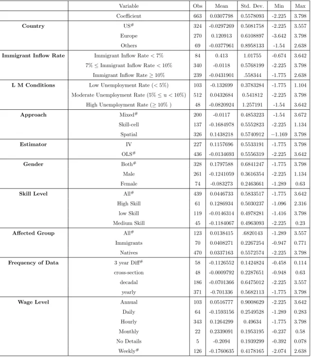
This thesis extends the existing literature on the response of labour markets to different types of economic shocks. First, we examine the effects of sector-specific fluctuations in job separation and job finding rates on the overall unemployment, sectoral allocation of labour and wages by solving a two-sector search and matching model with heterogeneous workers. The simulated results show how sector-specific shocks spill over the rest of the economy, causing workers to relocate between sectors in search of jobs. Inter-sectoral reallocation depends on the distribution of worker productivity in the affected sector. When an adverse shock hits a sector that attracts workers with relatively low productivity, the most productive among displaced workers move to compete for jobs in the sector with higher productivity. This offsets some of the increase in unemployment, subject to the ability of unaffected sector to employ additional workers. Next, we conduct meta-analysis to explain discrepancies between estimated effects of immigration shocks on wages in the literature. The results show that wage impact of immigration tends to be small in magnitude and negative significant. Labour market conditions at the period of study play a significant role in explaining the differences in measured impact. The estimates vary across countries and are related to the choice of modelling approach and estimators. Finally, we use EU-LFS dataset to analyse unemployment and labour market flows in Europe between 2006 and 2016. We identify the relative impact of shocks to job finding and separation rates on unemployment and investigate the role of socio-demographics, urbanisation and immigration status in shaping worker flow patterns in Europe. We find that over the studied period job losses accounted for three quarters of the rise in unemployment. The analysis of socio-demographic characteristics of the unemployed shows that young and less educated workers contributed the most to employment losses. Recent and intermediate immigrants in cities contributed to employment losses.
Contents
Introduction 10
1 The Multi-Sectoral Allocation of Workers 15
1.1 Introduction . . . 16
1.2 Data Facts for the US labour market . . . 20
1.3 Model . . . 24
1.3.1 Workers . . . 26
1.3.2 Firms . . . 28
1.3.3 Wage Determination . . . 28
1.3.4 Reservation Productivity . . . 29
1.3.5 Cut-Off Productivity Thresholds . . . 31
1.3.6 Ins and Outs of Employment . . . 34
1.3.7 Equilibrium . . . 36
1.4 Parametrization . . . 38
1.5 Baseline Case . . . 40
1.6 Simulations and Counterfactuals . . . 43
1.6.1 Simulations . . . 43
1.6.2 Counterfactuals . . . 50
1.7 Two-Sector Economy: Manufacturing and Construction . . . 52
1.8 Discussion . . . 55
1.9 Conclusion . . . 57
5
2 The Wage Effect of Immigration: A Meta-Analysis 66
2.1 Introduction . . . 67
2.2 Why do Estimates Differ? . . . 72
2.3 Selection of Studies and Construction of Dataset . . . 75
2.4 Meta-Regression Methodology and Results . . . 78
2.5 Publication Bias and P-hacking . . . 85
2.6 Robustness Check . . . 90 2.7 Discussion . . . 92 2.8 Conclusion . . . 96 2.9 Appendices . . . 99 2.9.1 Tables . . . 99 2.9.2 Figures . . . 105
3 Unemployment and Labour Market Mobility in Europe 107 3.1 Introduction . . . 108
3.2 Data Description and Summary Statistics . . . 114
3.3 Worker Flows . . . 118
3.4 Worker Flows by Socio-Demographic Groups . . . 122
3.4.1 Estimation Methodology . . . 125 3.4.2 Results . . . 126 3.5 Discussion . . . 132 3.6 Conclusion . . . 137 3.7 Appendices . . . 140 3.7.1 Tables . . . 140 3.7.2 Figures . . . 155
3.7.3 Countries in the Sample. . . 158
4 Concluding Remarks 159
List of Tables
1.1 Percent Change in Employment of Selected Sectors at Recent Recessions . . . 21
1.2 Reasons for Displacement in the Last Two Recessions . . . 22
1.3 Parameter Values . . . 39
1.4 Baseline Model Variables . . . 41
1.5 Aggregate Model Outcomes vs US Data . . . 41
1.6 Parameter Values for Manufacturing Sector . . . 53
1.7 Baseline Model Variables of Two Sectors Model Economy . . . 53
2.1 Sample of Studies . . . 99
2.2 Summary statistics of effect size corresponding to study features. . . 100
2.3 Marginal Effects . . . 101
2.4 Test for Publication Bias . . . 102
2.5 Tests for Evidential Value and p-hacking for published significant estimates at 5%. . 102
2.6 Tests for Evidential Value and p-hacking for published significant estimates at 1%. . 103
2.7 Tests for Evidential Value and p-hacking for published significant estimates at 10%. 103 2.8 Robustness Checks . . . 104
3.1 Summary Statistics . . . 140
3.2 Unemployment Rate (%) . . . 141
3.3 Europeanst andft . . . 141
3.4 Role of inflows and outflows in European unemployment. . . 141
3.5 st by Countries . . . 142
7
3.7 Europeanst by Socio-demographic Groups . . . 143
3.8 Europeanftby Socio-demographic Groups . . . 143
3.9 Europeanst by Urbanisation Level and Immigrant Groups . . . 144
3.10 Europeanftby Urbanisation Level and Immigrant Groups . . . 144
3.11 Contribution to Worker groups’ unemployment variance of changes in: . . . 145
3.12 Marginal Effects: Benchmark Case . . . 146
3.13 Marginal Effects: EU Transitions . . . 147
3.14 Marginal Effects: UE Transitions . . . 148
3.15 Marginal Effects of Interactions: EU Transitions I . . . 149
3.16 Marginal Effects of Interactions: EU Transitions II . . . 150
3.17 Marginal Effects of Interactions: UE Transitions I . . . 151
3.18 Marginal Effects of Interactions: UE Transitions II . . . 152
3.19 Marginal Effects: Benchmark Case (Robustness Checks) . . . 152
3.20 Marginal Effects: EU Transitions (Robustness Checks) . . . 153
List of Figures
1.1 US Average Unemployment Rate by Sectors . . . 20
1.2 US Average Wages by Sectors . . . 23
1.3 Simulating the Impact ofδ on Aggregate Model Outcomes. . . 45
1.4 Simulating the Impact ofαon Aggregate Model Outcomes. . . 47
1.5 Simulating the Impact ofδ andαon Aggregate Model Outcomes. . . 49
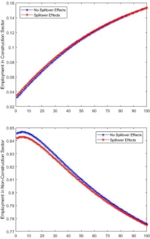
1.6 Counterfactuals: Spillover Vs No Spillover Unemployment . . . 50
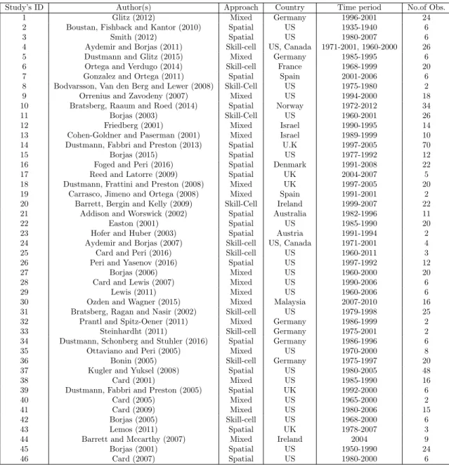
1.7 Counterfactuals: Spillover Vs No Spillover Employment in Construction and Non-Construction Sector . . . 52
1.8 Simulating the Impact ofδ andαon Two-Sector Economy. . . 54
2.1 Total Effect Sizes From All Primary Studies . . . 105
2.2 Sign and Significance of the Effect Sizes . . . 105
2.3 Funnel Plot For Publication Bias . . . 106
2.4 The Distribution of P-values for Significant Estimates . . . 106
3.1 Unemployment Rate (2006-2016) . . . 155
3.2 Inactivity Rate (2006-2016) . . . 155
3.3 European Unemployment, Job Separation and Job Finding Rates. . . 156
3.4 Changes in log inflow and outflow rates . . . 156
3.5 European Unemployment Rate by Socio Demographic Groups, Degree of Urbanisa-tion and MigraUrbanisa-tion Status. . . 157
9
Abbreviations
BLS Bureau of Labour Statistics
CES Current Employment Survey
CEPR Center for Economic Policy Research
CPS Current Population Survey
DWS Displaced Worker Survey
EU Employment to Unemployment
EU-LFS European Union Labour Force Survey
IV Instrumental Variable
JOLTS Job Openings and Labour Turnover Survey
MP Mortensen and Pissarides
NELP National Employment Law Project
OLS Ordinary Least Squares
SDC Socio-Demographic Characteristics
11
Labour market outcomes are very important for the welfare of any individual and are of funda-mental importance for the formation of public policies. Policy making relies heavily on realistic characterisation and representation of labour markets over time. The three chapters of this thesis are self-contained and contribute to our understanding of how labour markets respond to sector-specific fluctuations in job separation and job finding rates, migration and changing socio-demographics over time. This section summarises each of the three chapters.
The first chapter is entitled Multi-sectoral allocation of workers. This chapter evaluates the ef-fect of sector-specific shocks on the unemployment, allocation of labour across sectors and wages. It applies the two-sector equilibrium search model by Albrecht et al. (2009) to the US economy during 2006-2010, covering the period of Great Recession. The model is calibrated to the US construction and non-construction sectors. The motivation behind this chapter is that the 2008 recession caused the US national unemployment rate to increase from 5% in 2007 to about 10% in 2009. This increase in unemployment was linked to displacement of workers from sectors in which they were previously employed. The uneven distribution of job losses across industries caused struc-tural imbalances in the economy that required substantial movements of workers between sectors (Phelps 2008).
The results of the simulations show that when adverse shocks to job finding and job separation rates that are specific to the construction sector hit the economy, the unemployment levels of low and medium productivity workers in this sector increase while unemployment among high pro-ductivity workers in non-construction sector remains unchanged. While low propro-ductivity workers remain in the construction sector, some medium productivity workers move to the non-construction sector. For example, when job separation rate in the construction sector increases by 20% and job finding rate decreases by 15%, employment in non-construction sector increases by approximately 1.6% as medium productivity workers move to this sector for work. In the meantime, employment in construction sector decreases by 11% and the total unemployment in the economy increases by
10%. The average wages decrease by only 0.9%, suggesting wage stickiness. The results in this chapter indicate that relocation of medium productivity workers to non-construction jobs helps in reducing some of the increase in total unemployment. It helps in understanding that while sector-specific fluctuations in job finding and job separation rates increases the total unemployment in the economy, the movement of workers between sectors can also possibly reduce total unemployment as some displaced workers get re-employed in growing sectors. The results of the counterfactual exercise show that in the absence of spill-over effects, the increase in unemployment is lower than the case when there are spillover effects. This is because for any shock resulting in labor reallocation across sectors, the economy will take much longer to respond due to imperfect mobility in addition to the standard search friction causing higher unemployment rate. In case of no spill over effects, the employment in construction sector is lower and employment in non-construction sector is high.
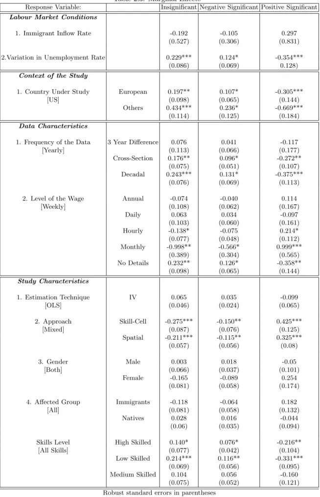
The second chapter is calledThe wage effect of immigration: A meta-analysis. Over the last three decades, there was a large body of literature assessing the wage effect of immigration. Yet existing evidence on whether immigration has a positive or negative effect on wages and if the impact is sig-nificant or not is still inconclusive. Therefore, this chapter aggregates 663 estimates of wage impact of immigration from 46 papers and evaluates the sign and significance of the effect of immigration through meta-analysis. The systematic differences in each study are classified in three categories: characteristics of the study, context of the study and labour market conditions. The estimation results show that the wage impact of immigration is generally small and negative significant. The results vary across countries and are related to the type of modelling approach and estimation spec-ification used. Studies using skill-cell approach tend to find positive significant impact as compared to mixed approach. The labour market conditions in a country play a significant role in explain-ing why wage impact of immigration varies from study to study. Bad labour market conditions i.e. high unemployment rate in the host country decrease the probability of finding positive signifi-cant results by 35% and increase the probability of finding negative signifisignifi-cant results by about 19%.
13
In meta-analysis literature, there is increasing concern that sample of studies suffer from researcher driven biases. It is also argued in recent research that selection bias is severe and prevalent in economics (Olken 2015, Broudeur et al. 2016, Christensen and Miguel 2018). The two widely recognised researcher driven biases are publication bias and p-hacking. Publication bias happens when authors, referees and editors prefer the publication of statistically significant results, while p-hacking occurs when authors influence their data and/or statistical analysis to produce significant results. In this chapter, the presence of publication bias is investigated using two tests suggested by Card and Krueger (1995) and Stanley et al. (2004). P-hacking is checked for by using a test suggested by Head et al. (2015). The results show that sample of studies collected for this meta-analysis do not suffer from researcher driven biases. The most important aspect of the meta-meta-analysis in this chapter is that it takes into account the economic conditions of a country when assessing the wage impact of immigration. It also provides a critical discussion of the wage impact of immigration by classifying study differences into three categories based on context of the study, labour market conditions and study characteristics.
The third chapter is calledUnemployment and labour market mobility in Europe. European Union is making progress to be viewed as a single economic area. A single labour market is one of the most flourishing policy areas of European Union’s integration and enlargement. A defiant feature of this single European labour market is the substantial variation in its unemployment rate over the years. Labour market dynamics literature since 1970s argue that changes in the stock of unemploy-ment are shaped by the flows of workers between employunemploy-ment and unemployunemploy-ment pools. Economic theory also highlights that different labour market groups play a significant role in contributing to unemployment variation through worker flows. Focusing on these three dimensions, this chapter evaluates the annual worker flows and socio-demographic composition of these flows in Europe to identify the contribution of job finding and job separation rates to the changes in the unemployment rate and to assess the importance of socio-demographics in shaping worker flow patterns in Europe. Using European Union labour force survey (EU-LFS), worker flows are calculated at the European
level. The European unemployment variance is decomposed into parts accounted for by changes in unemployment inflow and outflow rates and lastly, the correlation between the socio-demographic characteristics, immigration status, degree of urbanisation and worker flows is evaluated.
The results are as follows. Transitions from unemployment to employment are found to be less frequent over the years for Europe compared to the flows from employment to unemployment. The latter have significantly changed over time since 2006 and have not adjusted back to their initial levels. Unemployment outflow rate accounts for around 24% of the rise in unemployment while un-employment inflow rate accounts for around 73%. The estimation results show that male workers, less educated workers and young workers are affected the most as they have higher probability of job losses than other socio-demographic groups. Worker from Southern European countries (Spain, Greece and Portugal) have higher probability of employment to unemployment transition and lower probability of unemployment to employment transition than other regions. Recent and interme-diate immigrants are adversely effected as they increase the probability of job separation by 1.6% and 1.5%, respectively. For urbanisation groups, workers in town/suburbs and rural areas lower the job separation probability by 0.38% and 0.4%, respectively compared to workers in cities. The results also show that all three immigrant groups in towns and rural areas have lower job separation rates and higher job finding rates as compared to the workers in cities. The main contributions of this chapter are that it identifies the role of job finding and job separation rates in changing Euro-pean unemployment rate. It also provides a structural analysis of unemployment and worker flows by using annual gross data for calculations. This chapter also highlights the correlation between socio-demographic characteristics, degree of urbanisation of workers, their immigration status and worker flows.
15
Chapter 1
The Multi-Sectoral Allocation of
Workers
1.1
Introduction
The Great Recession has adversely affected the overall labour market and started problems in the housing and financial sectors. However, its impact was not the same across different sectors and industries. Because of the mortgage crisis and problems in the housing markets, the construction sector was among the most adversely affected. While the overall employment loss in the economy between December 2007 and January 2009 was 6%, construction went down by 13.7% over the same period. In contrast, employment in education and health services increased by almost 2.2%.1
In addition, job losses were unevenly distributed among industries with different average wages. About 60% of all job losses recorded during recession originated in industries that paid average hourly wages ranging from 14 and 21 dollars per hour, such as construction and retail trade. The industries that paid average hourly wage of 21.14 to 54.55 dollars (such as health and education, professional and business services) contributed 19 percent to the job losses. 2 Statistics from Dis-placed Workers Survey (DWS, 2010) show that about 1.1 million workers in the construction sector lost their jobs. This accounted for 16% of the total displaced workers in the US. The main reasons reported for employment losses were insufficient work, plant and vacancy closure. Only 44% of these workers were able to get re-employed, with 23% finding work in other sectors. The average wages in the economy generally remained rigid throughout the recession. Fallick et al. (2016) assessed wage rigidity in the US during the Great Recession and reported no evidence that the high degree of labour market distress reduced the amount of downward nominal wage rigidity. Average hourly wages for several sectors (such as construction, manufacturing, retail, education and health services) were rigid during this time period.
The statistics above indicate that during the Great Recession, workers were displaced from con-struction sector and were re-employed to different industries. One aspect of changing labour market dynamics of a particular sector during a recession is that it can have spillover effects on other sectors
1Source: The Recession of 2007-2009: Bureau of Labour Statistics (BLS) Spotlight on Statistics.
17
or on the economy as a whole. These spillover effects due to intersectoral reallocation of workers in search of employment opportunities in one sector may contribute to unemployment changes in the economy. It is therefore important to understand whether the movement of workers between sectors explains the unemployment dynamics. In this paper, I examine the impact of sector-specific shock on the overall unemployment as well as unemployment dynamics for each worker type, employment levels in construction and non-construction sectors, distribution of workers across the sectors and average wages. I examine how the shocks experienced by a sector with low productivity propagate to other sectors of the economy, and evaluate the response of sector-specific and economy-wide employment levels and wages to these shocks. I also explain the role played by worker productivity in the sectoral allocation of workers.
In order to assess the spillover effects of an adverse shock in one sector on the labour market outcomes in the economy, I set up a two-sector equilibrium search and matching model which ex-tends the canonical Mortensen and Pissarides (1994, MP) search and matching framework and is similar to the one developed by Albrecht, Navarro and Vroman (2009). I solve the model to derive the worker productivity thresholds that determine the distribution of workers between the two sec-tors and reservation productivity schedule of each worker type. These productivity thresholds are used to determine steady state employment in the two sectors and unemployment for each worker type and overall economy. The model is calibrated to pre-recession (2007) US construction and non-construction sectors to ensure that the baseline labour market matches the data.
After the baseline economy is set up, I treat the fluctuations in job separation and job finding rates in construction sector as indicators of adverse shock in this sector during a recession and run simulations to assess how these sector-specific shocks propagate to the rest of the economy. This is because job finding was low in construction sector due to low re-employment rates and job separation rates were high due to workers displacement in this sector. Taking various combinations of job finding and separation rates, I examine the effect of shocks on unemployment of each worker
type and overall economy, employment in the two sectors and wages in the model economy.
I run three sets of simulations. In the first case, I increase job separation rate while keeping the job finding rate constant. In the second case, I change the job finding rate and keep job separa-tion rate constant. In the third case, I change both of them simultaneously. As a result of the first case, the employment dynamics start to change in the construction sector as unemployment for low and medium productivity workers increases by 15% and 9% respectively. In the non-construction sector, while unemployment remains unchanged, employment starts to increase by 1% as medium productivity workers move to this sector to find work. The overall unemployment in the economy increases by 5% but it is not as severe as the unemployment levels of low and medium productivity workers. This is because some of the increase in the overall unemployment is offset by medium productivity workers finding work in the non-construction sector. When job finding rate starts to decrease, unemployment for low and medium productivity workers in construction sector increases by 20% and 10% respectively. The overall unemployment in the model economy increases by 6%. Employment in non-construction sector increase by 1.2%. In the final case, when job separation rate increases and job finding rate decreases, unemployment for low and medium productivity workers in construction sector increases by 30% and 15% while overall unemployment increases by 10%. Employment in construction sector decreases by 11% and it increases in non-construction sector by 1.6%. The results of the counterfactuals indicate that sector-specific shocks do have spillover effects on other sectors and the economy, as they tend to increase unemployment rate and causes workers to relocate to other sectors to find work. This reallocation of workers depends on the productivity levels of workers.
After the simulations, I run counterfactual exercise to quantify how much unemployment in the model will change in the absence of the spillover effects. The results show that incase of no spillover effects, unemployment in the model is lower, employment in construction sector is lower and em-ployment in non-construction sector is high. Manufacturing sector is closer in terms of skills to
19
construction sector, I assume the model economy has two sectors only; construction and manufac-turing. The baseline and simulation results show that unemployment is higher for this hypothetical economy.
This paper contributes to the literature that examines the impact of inter-sectoral mobility of workers on the levels of unemployment in the economy, especially during the Great Recession, and tests the sectoral shift hypothesis of Lilien (1982). It was reported in this study that the structural changes in the US sectors in the 1970s caused the equilibrium unemployment rate to fluctuate by about 3%. Alvarez and Shimer (2011) analyse theoretical properties of the labour market equilibrium in an economy with a continuum of industries and rest unemployment, which allows unemployed workers to wait for better prospects in their own industry instead of automatically engaging in search activities. Chang (2011) and Pilossoph (2012) approach sectoral reallocation by using multi-sectoral models based on MP (1994) to estimate the effects of sectoral reallocation on aggregate unemployment and wages. Carilla-Tudela and Visschers (2013) create a multi-sectoral MP model and examine the interactions between rest, search and reallocation unemployment. I extend this literature further by examining the response of sector-specific shock on unemployment of worker types, employment in each sector and wages.
The paper is organised as follows. In the next section, data facts about the US labour market during 2007-2009 recession are reviewed. In section 1.3, I will set up and solve the two sector search and matching model. Section 1.4 explains the data and the calibration strategy of parameters of the model. Section 1.5 then explains the baseline case, while section 1.6 will present the simula-tions and counterfactuals of the model. Section 1.7 calibrates the model to US construction and manufacturing sector only. Section 1.8 provides the discussion and section 1.9 concludes.
1.2
Data Facts for the US labour market
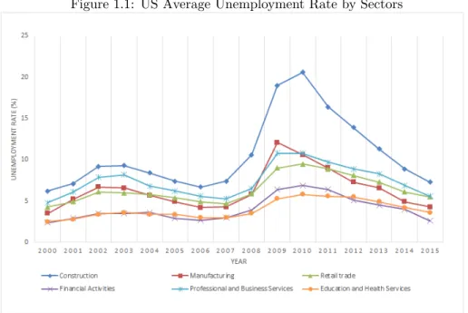
In this section, I review the data facts for the US labour market to highlight the role played by different sectors in changing employment dynamics of the overall economy during the Great Re-cession. The US labour market has been deeply affected by the Great Recession of 2007-2009. Unemployment rate was one of the main indicators of 2008 crisis as it increased from 5% in 2007 to about 10% in 2009. Unemployment by industry is defined as the number of workers who are out of work and had held their last jobs in the specific industry. In order to understand the role played by each sector in changing labour market dynamics of the US economy, unemployment rate for different sectors is extracted from CPS data and is shown in Figure 1.1 below. Unemployment was generally the highest for goods producing industries as shown in Figure 1.1. Construction sector
Figure 1.1: US Average Unemployment Rate by Sectors
Data source: US Bureau of Labour Statistics (BLS): Labour Force Statistics from the Current Population Survey.
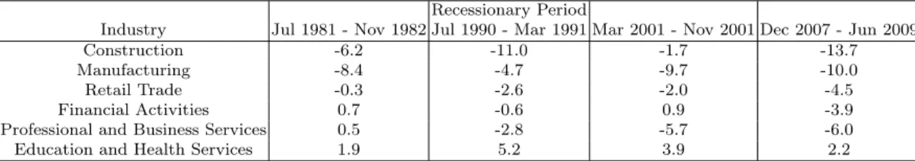
suffered from the largest increase in its unemployment rate as it increased from 10% in 2008 to about 18% in 2009. The job losses during this crisis were larger than in the previous recessions. Table 1.1 shows the percentage change in employment of six main industries in the US during the
21
last four recessions.3 Manufacturing sector experienced large employment losses during all four
re-cessions. Barring the 2001 recession, the construction sector experienced high levels of employment losses in all others. The 2007-2009 recession was typical in this regard, with construction and man-ufacturing both experiencing their largest percentage declines in employment of 13.7% and 10.0% respectively. The employment losses in the US construction sector were the highest among all the
Table 1.1: Percent Change in Employment of Selected Sectors at Recent Recessions Recessionary Period
Industry Jul 1981 - Nov 1982 Jul 1990 - Mar 1991 Mar 2001 - Nov 2001 Dec 2007 - Jun 2009
Construction -6.2 -11.0 -1.7 -13.7
Manufacturing -8.4 -4.7 -9.7 -10.0
Retail Trade -0.3 -2.6 -2.0 -4.5
Financial Activities 0.7 -0.6 0.9 -3.9
Professional and Business Services 0.5 -2.8 -5.7 -6.0
Education and Health Services 1.9 5.2 3.9 2.2
Data source: Current Employment Survey (CES)
sectors. Data extracted from Current Employment Survey (CES) Highlights (2007-2008) shows that during 2007-2008, construction sector lost 195,000 jobs, with the residential components account-ing for the decline and reflectaccount-ing the continuaccount-ing difficulties in the housaccount-ing market. Few industries attracted as much attention during the recent recession as financial activities, which experienced a 3.9% reduction in employment. Before 2007, the only recession since 1939 to see job losses in financial activities was that of 1990-1991. Employment increased in education and health services during the recent recession. In fact, employment in this sector has increased for more than 30 years at all stages of the business cycle. Employment in education and health services has decreased in only 1 of the 12 recessions that have occurred since 1945.4 This suggests that workers were moving
to other sectors after suffering from job losses in their initial sectors. These sector-specific job losses and limited employment opportunities led to displacement of workers from these sectors.
The Bureau of Labour Statistics defines a displaced worker as persons 20 years of age and older who lost or left job because their plant or company closed or moved, there was insufficient work for them to do, or their position or shift was abolished. Displaced worker survey (DWS 2010) reported that
3Since the recessions vary in length, the percentages are measured across different number of months for recession
and then they are transformed to annual percentages.
around 6.8 million workers in the US were displaced from their jobs during the 2007-2009 recession. The number of displaced workers in construction sector were more than 1.1 million. In 2010, the re-employment rate of displaced workers in this sector was 44% with only 21% finding employment in the same sector. The other 23% were re-employed in other sectors.5 Construction sector at the time made up about 7% of the US workforce. These figures indicate that with low re-employment rates and accounting for 16% of the total displaced worker group in the US, construction sector was one of the adversely effected sectors in terms of employment losses, with many workers finding employment in other sectors.
Table 1.2: Reasons for Displacement in the Last Two Recessions Year
Reasons 2002 2010
Insufficient work 26% 43%
Plant or company closed/moved 47% 31%
Position or shift abolished 27% 26%
Data source: U.S. Bureau of Labour Statistics. 2010. News Release: Worker Displacement: 2007-2009.
Reasons of displacement during the Last Two Recessions using data extracted from DWS are re-ported in Table 1.2. During the Great Recession, most workers lost their jobs due to the lack of full time job opportunities - 43% of the workers were displaced due to insufficient work. Job separation was also one of the main reasons for employment losses as about 31% of the workers lost their jobs due to plant or company closing and 26% were separated from their jobs because their posts were abolished. This highlights the fact that workers were becoming unemployed from their respective sectors due to low job finding rate in the form of low re-employment rates within the same sector and high job separation rate in the form of company closure, insufficient work and termination of jobs.
Elsby et al. (2013) report that real wages are procyclical but the degree of procyclicality varies
5Data Source: U.S. Bureau of Labor Statistics. 2010. News Release: Worker Displacement: 2007-2009.
23
across recessions. US distributions of year-to-year nominal wage change show many workers report-ing zero change (suggestreport-ing wage stickiness) and many reportreport-ing nominal reductions (suggestreport-ing wage flexibility). The wage data for different industries have been collected from the CPS dataset
Figure 1.2: US Average Wages by Sectors
Data source: CPS.
for 2006-2015. The respondents were asked questions about their occupation and industries in which they are working currently and in which they have worked a year before. For the purpose of this study, the nominal wage variables for workers in each of the five industries were created. The wages were then converted into real wages by using annual CPI. Figure 1.2 shows the average real wage for each year between 2006 and 2015 for five different industries in the US. Reductions in the growth of wages and salaries typically began during recessions and continued afterwards as well. There has been a change in the average real wages of workers in professional and business services and the finance sectors over the years but on average, the wage growth slowed down during the Great Recession. Wages in the finance sector were more volatile, but showed no growth. Furthermore, even though there has been a decrease in employment in manufacturing and construction sectors in 2007-2009 recession, there is no significant change in the wages of these sectors.
These data facts from above show that during the Great Recession, some sectors (for example, construction) were adversely affected in terms of high unemployment and low re-employment rates due to high job separations and low job findings. The unemployed workers displaced from these sectors moved to other sectors to find work. On the other hand, there are some sectors where unemployment levels increased by small amount and/or are more or less the same before and after the Great Recession (for example, retail trade, professional and business services). In some sec-tors, unemployment has decreased during the great recession (for example, education and health services). The movement of displaced workers from construction sector to these sectors may have caused employment in these latter sectors to increase (for example, retail trade, education and health services). These data figures help to motivate the idea of worker reallocation between the sectors of economy in response to the shocks that originate in a specific sector which in turn may contribute to the changing unemployment rate in the whole economy.
1.3
Model
The model in this paper is based on the search and matching framework developed in MP (1994), which is extended to an economy with two sectors and heterogeneous workers. The two sectors of the economy differ in the work opportunities that they can offer and workers have different relative productivities in the two sectors. Similar approach has been previously developed and used in other two-sector settings, including formal versus informal and public versus private sectors (Albrecht et al. 2009, 2018). I use a simplified version of the model developed by Albrecht et al. (2009) without taxes, and apply it to the US construction and non-construction sectors.
In the model, the two sectors represent the US construction and non-construction. A shock to one particular sector takes place which spreads throughout the economy. Construction sector is chosen as an adversely affected sector because the empirical facts of the previous section show that this sector was hit harder than other sectors by the 2008 recession in terms of job loss and low
25
re-employment levels. The increase in the housing prices through various mechanisms caused a sharp reduction in construction activity. This led to significant job losses in this sector and the need to absorb unemployed workers in other sectors (Valleta et al. 2008).
Time is continuous, and the labour market is populated by a unit mass of risk neutral, infinitely lived workers who discount the future at rate r. Workers can be either unemployed or employed in one of the two sectors. They can move between the states of employment in construction sec-tor, employment in non-construction sector and unemployment. Immediate transitions between the jobs in two sectors are not allowed. Such transitions may only happen through the state of unemployment. Workers differ in the maximum productivity that they can achieve, denoted byy. Productivity is i.i.d. across the unit measure of workers and is described by a continuous proba-bility densityf(y),0 ≤y ≤1. Worker types are determined by dividing productivities y in three intervals, determined by two threshold levels. These thresholds are used to identify the distribution of workers across construction and non-construction sectors. The labour market frictions are mod-elled using a standard matching function. Workers and firms who meet form a match if and only if the joint surplus generated by the match is higher than the sum of the values of their respective outside options. Wages in non-construction sector are determined by Nash bargaining. Following the literature, I assume the free vacancy entry.
The two sectors in the model work in the following way. Workers employed in the construction sector receive flow income ofy0. They meet vacancies at the rateα, whereαis the exogenous job finding
rate in the construction sector. Construction jobs are destroyed at exogenous rateδ. This sector is assumed to be low skilled so the least productive workers in the economy do not find it profitable to work in non-construction sector. Employed workers in non-construction sector receive wagew
which depends on worker’s productivity level. The unemployed workers in non-construction sector find jobs at a ratem(θ), wherem is the matching function andθ is the labour market tightness. When the matches are formed, all workers start non-construction jobs at their maximum potential
productivity levels. Later matches receive exogenous productivity shocks that arrive at Poisson rate
λand change the actual productivity of workers in the match toy0. Productivity shocks are i.i.d. drawn from a continuous densityg(y0)/G(y) for 0≤y0 ≤y, whereG(y) is a continuous distribution and 0≤y≤1. The realised productivityy0 is restricted to be less than or equal toy because we assume that worker’s current productivity does not exceed his type.
If a series of productivity shocks pushes y0 so low that the match surplus becomes less than the sum of the outside options, worker and firm will decide to end the match. The threshold value of productivityy0 that determines the point of match destruction defines the reservation productivity of a worker of typey and is denoted by R(y). The reservation productivity R(y) is determined endogenously in the model for each worker type. Ify0 ≤R(y), the match breaks with probability
G(R(y))/G(y). IfR(y)≤y0 ≤y, the productivity changes to y0 and the match survives with the
probability 1−G(R(y))/G(y). The reservation productivity also determines the lowest level of worker’s productivity type that a firm would be willing to hire.
With all the model assumptions, I set up the value functions for unemployed and employed workers in the two sectors. These will then be used to derive wage schedule for non-construction sector, reser-vation productivity schedule, cut-off productivities that identify the sector in which each worker type works. The employment levels in the two sectors and unemployment level in the economy will be determined using the derived productivity levels and model’s assumptions on the sectoral allocation of each worker type.
1.3.1
Workers
Unemployed workers receive a flow benefitb, and face a chance to meet vacancies in both construc-tion and non-construcconstruc-tion sectors. The value of unemployment for a worker of type y is denoted
27
byU(y) and is given by:
rU(y) =b+αmax[No(y)−U(y),0] +m(θ)max[N1(y)−U(y),0], (1.1)
whereαis the job finding rate in construction sector andm(θ) is the matching function. At the rate
α, a worker receives an opportunity to work in the construction sector and, if the match is formed, gains the flow value of No(y)−U(y), which is the difference between the values of employment
and unemployment in construction, U(y). Non-construction jobs arrive at the rate m(θ) and, if the match is formed, yield the difference between the values of employment and unemployment in non-construction sector,N1(y)−U(y). The value of employment in construction sector for a worker
of typey is given by:
rNo(y) =yo+δ[U(y)−No(y)]. (1.2)
Equation (1.2) states that a worker employed in construction sector gets a flow income ofy0while
employment lasts,y0 ≥b. At the rateδ, he loses his job and gets a capital gain ofU(y)−No(y).
The value of employment in non-construction sector for a worker of typeywith current productivity levely0,N 1(y0, y) is given by: rN1(y0, y) =w(y0, y) +λ G[R(y)] G(y) [U(y)−N1(y 0, y)] +λ Z y R(y) [N1(x, y)−N1(y0, y)] g(x) G(y)dx, (1.3)
Equation (1.3) states that a worker employed in non-construction sector gets a wagew(y) from the match. At the rateλ, a shock that affects worker’s realised productivity arrives. This shock either destroys the job with the probability G[R(y)]
G(y) or shifts the productivity to a new level in the range
R(y) ≤ y0 ≤y, in which case a worker stays employed but the value of employment changes to
1.3.2
Firms
Let J(y0, y) be the value of a filled job for a firm that employs a worker of type y with current productivity levely0 and it is given by:
rJ(y0, y) =y0−w(y0, y) +λG[R(y)] G(y) [V −J(y 0, y)] +λ Z y R(y) [J(x, y)−J(y0, y)]g(x) G(y).dx (1.4)
Equation (1.4) states that a firm receives a flow output of y0 and pays a wage of w(y0, y). At the rate λ, a productivity shock arrives which causes the job to become vacant with the probability
G[R(y)]
G(y) . If the new productivity level is in the rangeR(y)≤y
0≤y , the match survives but firm’s
value changes toJ(x, y). Let V be the value of a vacancy and it is defined as:
rV =−c+m(θ)
θ max[J(y)−V,0]; (1.5)
Equation (1.5) states that the vacancy is advertised at a cost of c and if filled gives firm a capital gain ofJ(y)−V. One of the important and fundamental equilibrium assumptions in MP (1994) is that there is free entry of vacancies i.e. V = 0. This helps in determining the equilibrium value of
θ.
1.3.3
Wage Determination
Wages in non-construction sector are determined through Nash bargaining. With worker’s bargain-ing parameterβ and the equilibrium condition of free entryV = 0, the joint surplus from a match can be written as:
maxw(y0,y)[N1(y, w)−U(y)]βJ(y, w)1−β
29
of the two and simplifying it:
r[βJ(y)−(1−β)N1(y)] =βy−w(y0, y)−λ G[R(y)] G(y) [βJ(y) + (1−β)(U(y)−N1(y))] +λ Z y R(y) [β(J(x, y)−J(y))−(1−β)((U(y)−N1(y))] g(x) G(y)dx (1.6)
The surplus of a match is defined as the sum of the gain of the firm and worker being in a match relative to not being in a match. It is assumed that the wage is set such that the total match sur-plus is shared between the worker and firm according to the Nash-bargaining solution with share parameterβ. The surplus sharing rule is as follows:
(1−β)N(y)−(1−β)U(y) =βJ(y)
−(1−β)U(y) =βJ(y)−(1−β)N(y)
(1.7)
Putting (1.7) in the equation (1.6) and simplifying it:
w(y0, y) =βy+r(1−β)U(y) (1.8)
Equation (1.8) determines the wage paid to the workers in non-construction sector. It states that the wage is a weighted average of productivity and the flow value of unemployment with the weights beingβ and 1−β, respectively.
1.3.4
Reservation Productivity
When a productivity shock is realised, workers and firms separate if worker’s productivity level is less than reservation productivity R(y). R(y) is derived using zero surplus sharing rule which states that a match between the firm and a worker with current productivity level equal toR(y) will generate zero profits and is given as:
Worker with current productivity of R(y) will equally value employment and unemployment i.e.
N(R(y), y) =U(y). So the surplus sharing rule is equal to:
J(R(y), y) = 0
The substitution of wage equation (1.8) in (1.4) which is the value function of a filled job for a firm and using the fundamental equilibrium condition is given by free entry of vacancies i.e. V=0 which gives: (r+λ)J(y0, y) = (1−β)y0−r(1−β)U(y) +λ Z y R(y) J(x, y)g(x) G(y)dx (1.9)
Evaluation of equation (1.9) aty =R(y) i.e. when the current productivity of a worker equals his reservation productivity, and using the zero surplus sharing ruleJ(R(y), y) = 0 gives:
0 = (1−β)R(y)−r(1−β)U(y) +λ
Z y
R(y)
J(x, y)g(x)
G(y)dx (1.10)
Solving equation (1.9) and (1.10) simultaneously gives:
y−R(y) = (r+λ) (1−β)J(y
0, y) J(y0, y) =(1−β)(y−R(y))
(r+λ) (1.11)
Substitution of (1.11) in equation (1.9) and simplification gives:
(r+λ)J(y0, y) = (1−β)y0−r(1−β)U(y) +λ(1−β) (r+λ) (y−R(y))− λ(1−β) (r+λ)G(y) Z y R(y) G(x)dx
Evaluating the equation above at y’=R(y) at J(R(y),y))=0: and solving forR(y)
R(y) =
G(y)r(r+λ)U(y)−λ[Ry
R(y)(1−G(x))dx−(1−G(y))y]
31
For any value of y, there is a corresponding R(y). A higher y will increase outside options of a worker, i.e. U(y) is increasing in y. This causesR(y) to increase but the final term in equation (1.12) is decreasing iny which suggests thatR(y) decreases. Hence which of these effects onR(y) is higher depends on the parameter values.
1.3.5
Cut-Off Productivity Thresholds
The threshold of the productivity levels that identify whether the worker works in the construction or non-construction sector are such that a worker with productivity levely≤y∗will not be able to work in the non-construction sector. This is because non-construction sector consists of high skilled workers on average so low productivity workers do not possess the necessary skill set to work in this sector. Similarly, workers withy≥y∗∗will not find it worthwhile to work in the construction sector because becoming unemployed in non-construction sector yields them more benefit than moving to the construction sector to find work.
There are two threshold levels of worker types. Workers withy < y∗ are low productivity workers and will only work in construction sector. Workers with y∗ ≤ y ≤ y∗∗ are medium productivity workers and they can work either in construction or non-construction sector depending on any job offer that comes along their way. Workers with y > y∗∗ are high productivity workers who will only work in non-construction sector. Using these characteristics of worker types, I derive the two cut-off productivity levels. First we consider worker’s cut-off productivity level y∗. The worker of this type is indifferent to being unemployed or being employed in non-construction sector i.e.
U(y∗) =N
1(y∗). Hence his value functions can be written as:
rU(y∗) =b+α[No(y∗)−U(y∗)]
N0(y∗) =
y0+δU(y∗)
r+δ
Substituting the value ofN0(y∗) in rU(y∗) and simplifying it:
rU(y∗) =b(r+δ) +αy0
r+δ+α (1.13)
Equation (1.13) is the unemployment value for all workers withy ≤y∗ and it depends on the job finding rateαand job separation rateδ. Next we substituteN1(x, y) out of the following surplus
sharing rule:
N(x, y) = β
1−βJ(x, y) +U(y)
and substitute it in equation (1.3):
rN1(y∗) =w(y∗) +λ G[R(y∗)] G(y∗) [U(y ∗)−N 1(y∗)] +λ Z y∗ R(y∗) [ β 1−βJ(x, y ∗) +U(y∗)−N 1(y∗)] g(x) G(y∗)dx Now usingU(y∗) =N
1(y∗) and simplifying it using wage equation (1.8):
rN1(y∗) =βy∗+r(1−β)U(y∗) + λβ (r+λ)G(y)[ Z y∗ R(y∗) (G(y∗)−G(x))dx] Solving fory∗ usingU(y∗) =N1(y∗):
y∗=b(r+δ) +αy0 r+δ+α − λ (r+λ)G(y)[ Z y∗ R(y∗) (G(y∗)−G(x))dx] (1.14) Equation (1.14) shows that y∗ depends on rU(y∗) so R(y∗) also depends on rU(y∗). Next, a high productivity worker will only accept non-construction sector jobs and is indifferent between unemployment and construction sector job offers, so for himU(y∗∗) =N0(y∗∗). Using this condition
33
rU(y∗∗) =b+α[No(y∗∗)−U(y∗∗)] +m(θ)max[N1(y∗∗)−U(y∗∗)]
rU(y∗∗) =b+m(θ)max[N1(y∗∗)−U(y∗∗)]
SinceU(y∗∗) =N0(y∗∗) so we know fromrN0(y∗∗):
rN0(y∗∗) =y0
and
rU(y∗∗) =rN0(y∗∗) =y0 (1.15)
Equation (1.15) shows that unemployment valueU(y∗∗) is equal to the flow incomey0for all workers
withy≥y∗∗ So: y0=b+m(θ)max[N1(y∗∗)− y0 r ] N1(y∗∗) = y0(r+m(θ))−rb rm(θ) (1.16)
Equation (1.16) shows that the value of employment for workers with y ≥ y∗∗ depends on the matching functionm(θ) and labour market tightnessθ. SubstitutingN1(x, y∗∗) from surplus sharing
rule into equation (1.3) and simplifying it using wage equation (1.8), value ofN1(y∗∗) and using
equation (1.11) to replaceJ(x, y∗∗): (r+λ)y0(r+m(θ))−rb m(θ) =βy ∗∗+r(1−β)U(y∗∗)+λU(y∗∗)+ λβ (r+λ)G(y∗∗)[ Z y∗∗ R(y∗∗) (G(y∗∗)−G(x))dx] Simplifying in terms ofy∗∗: y∗∗=y0+ (rG(y∗∗) +λ) (y0−b) βm(θ)G(y∗∗)− λ (r+λ)G(y∗∗)[ Z y∗∗ R(y∗∗) (G(y∗∗)−G(x))dx] (1.17)
y∗∗ depends on them(θ), reservation productivityR(y∗∗) and model parameters.
1.3.6
Ins and Outs of Employment
In order to derive the employment rates for the two sectors and unemployment rates for different worker types and overall economy, the steady state conditions of the model are used. Letu(y) be the fraction of time of unemployment for worker typey,nC(y) be the fraction of time of employment
for workers in construction sector andnN C(y) be the fraction time of employment for workers in
non-construction sector. The sum of these three equals one and can be written as:
u(y) +nC(y) +nN C(y) = 1 (1.18)
The steady state condition for low productivity workers in construction sector is that flow into em-ployment equals the flow into unemem-ployment. So the steady state unemem-ployment and emem-ployment for workers of typey < y∗ is equal to:
u(y) = δ δ+α (1.19) nC(y) = α δ+α (1.20) nN C(y) = 0 (1.21)
nN C(y) = 0 because a low productivity worker will not be able to work in non-construction sector.
For workers of typey∗≤y≤y∗∗, the steady state conditions are such that the employment inflow in construction sector is equal to outflow into unemployment in the same sector:
αu(y) =δnC(y) (1.22)
35
m(θ)u(y) =λG[R(y)]
G(y) nN C(y) (1.23)
and
nN C(y) = 1−u(y)−nC(y) (1.24)
So from solving equation (1.22), (1.23) and (1.24) simultaneously, we get the employment and unemployment rates which are as follows:
nC(y) = αλG[R(y)] δm(θ)G(y) +λ(δ+α)G(R(y)) (1.25) u(y) = δλG[R(y)] δm(θ)G(y) +λ(δ+α)G(R(y)) (1.26) nN C(y) = δm(θ)G(y) δm(θ)G(y) +λ(δ+α)G(R(y)) (1.27) For workers of typey > y∗∗, the steady state condition is such that the flow into employment in non-construction sector is equal to outflow into unemployment in the same sector:
m(θ)u(y) =λG[R(y)]
G(y) nN C(y) which can be rewritten as:
m(θ)u(y) =λG[R(y)]
G(y) [1−u(y)] (1.28)
and we know that such workers will not work in the construction sector so the employment rate for these workers in construction sector can be written as
hence simplifying equations (1.24), (1.28) and (1.29) in terms ofu(y) andnN C(y): u(y) = λG[R(y)] m(θ)G(y) +λG(R(y)) (1.30) nN C(y) = m(θ)G(y) m(θ)G(y) +λG(R(y)) (1.31)
The total unemployment in the economy will be derived by the following:
u= Z y∗ 0 u(y)f(y)dy+ Z y∗∗ y∗ u(y)f(y)dy+ Z 1 y∗∗ u(y)f(y)dy (1.32) Intuitively, in equilibrium, workers will be sorted in the two sectors based on their types, y. High productivity workers are more likely to take jobs in non-construction sector, while low productivity workers are more likely to take construction sector jobs, and medium productivity workers will take both. In addition to compositional effects, changes in model parameters affect the steady state distributions of workers among sectors, affecting also the distributions of wages across non-construction sector.
1.3.7
Equilibrium
The fundamental equilibrium condition is given by free entry of vacancies i.e. V=0. So:
c=m(θ)
θ max[J(y
0, y),0] (1.33)
We need to take into account that the density of types among the unemployed is contaminated in the sense that the distribution of types among the unemployed is affected by the different transition rates to and from unemployment by worker types. Letfu(y) be the density of types among unemployed
workers. The can also be written as:
37
The eexpression above states that the distribution of types among the unemployed, fu(y), can
be written as the type-specific unemployment rate, u(y), times the distribution function, f(y) normalised by the overall unemployment rate in equation (1.32). Using the above expression and replacing the value ofJ(y0, y) from (1.11), equation (1.33) becomes:
c= m(θ) θ (1−β) Z 1 y∗ (y−R(y)) (r+λ) u(y)f(y) u dy (1.34)
Equation (1.34) takes into account the fact thatJ(y)<0 fory < y∗, i.e., some contracts do not lead to a match. θ can be solved numerically given the assumed functional forms for the distribution functions, F(y), G(y) and for the matching function, m(θ) and values for exogenous parameter r
andλ. Normalising the total labour force to unity, an equilibrium is labour allocationsu(y),nC(y),
nN C(y) , set of value functionsNo(y),N1(y0, y),J(y0, y) andU(y), reservation productivity function
R(y), wagesw(y0, y) such that:
1. free entry condition holds in the economy and satisfies equation (1.34).
2. matches are completed and dissolved if and only if it is in the mutual interest of the worker and firm to do so.
3. the steady state condition holds which implies that the evolution of employment for three worker types follows equations (1.20) (1.21) (1.25), (1.27) (1.29) and (1.31) in the two sectors while
4. evolution of unemployment for three worker types and overall economy follows equations (1.19), (1.26) and (1.30) and (1.32).
5. workers of typey < y∗ do not find work in non-construction sector with cut-off productivity thresholdy∗satisfied by equation (1.14) and
6. workers of typey > y∗∗do not work in construction sector with cut-off productivity threshold
7. reservation productivity schedule follows equation (1.12) and differs for each worker type.
1.4
Parametrization
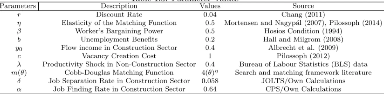
The model parameters, discount rater, elasticity of the matching function η, unemployment bene-fitsb, wage bargaining power parameterβ, flow incomey0, vacancy creation costc, Poisson rate at
which productivity shock arrivesλ, job finding rateαand job destruction rate δ need to be cali-brated in order to solve for the productivity thresholds, reservation productivities, non-construction wage distribution, employment and unemployment values for each sector. In this section I calibrate the model to US construction and non-construction sectors before great recession (i.e. in year 2007) using data from multiple sources. In order to analyse the effects of job separation and job finding rates, I fix several model parameters according to their values used in the literature and from other sources. The model parameter values are summarised in Table 1.3 and discussed below.
The parameter values in the model are chosen to produce results for the baseline case of the model that are consistent with the US economy. First, I choose the discount rate ofr= 0.04 and set the value of elasticity of matching function equal to η = 0.5. This value ofη = 0.5 is chosen from Mortensen and Nagypal (2007) and Pilossoph (2014) since they use data on vacancies and un-employment levels from CPS data to estimate the elasticity of the Cobb-Douglas matching function.
The worker’s bargaining power parameter β is set equal to the elasticity of matching function so that Hosios (1990) condition holds. This condition requires that the match surplus be divided between the workers and firms to properly compensate for their search decisions. More precisely, worker’s (or firm’s) share of the match surplus should be equal to their share of contribution in a match (Mangin and Julien 2018). A broad range of search models apply this condition (for ex-ample, Rogerson, Shimer, and Wright 2005; Pilossoph 2012; Wright, Kircher, Julien, and Guerrieri 2017). For this condition to hold, the elasticity of match function and Nash bargaining parameter are assumed to be equal to each other.
39
The value of the unemployment benefits is set as b = 0.2 and is taken from Hall and Milgrom (2008) who state that b is essentially a replacement rate, the fraction of normal earnings paid as the typical unemployment benefit and while some workers receive a substantial fraction of their earlier wages as benefits, many features of the system limit the effective rate. They estimate b=0.2 as a reasonable figure of unemployed benefits from the the lower (12%) and the upper bound (36%) of ratio of benefits paid to previous earnings that are calculated in the literature (Hall, 2006 and Anderson and Meyer, 1997).
I set the flow income to y0 = 0.4, and vacancy creation cost to c = 1, λ = 0.4 and assume a
Cobb-Douglas function of the formm(θ) = 4(θ)η from the search and matching literature so that
the model economy is an approximate of the US data.
Table 1.3: Parameter Values
Parameters Description Values Source
r Discount Rate 0.04 Chang (2011)
η Elasticity of the Matching Function 0.5 Mortensen and Nagyp´al (2007), Pilossoph (2014)
β Worker’s Bargaining Power 0.5 Hosios Condition (1994)
b Unemployment Benefits 0.2 Hall and Milgrom (2008)
y0 Flow income in Construction Sector 0.4 Albrecht et al. (2009)
c Vacancy Creation Cost 1 Pilossoph (2012)
λ Productivity Shock in Non-Construction Sector 0.4 Bureau of Labour Statistics (BLS) data
m(θ) Cobb-Douglas Matching Function 4(θ)η Search and matching framework literature
δ Job Separation Rate in Construction Sector 0.058 JOLTS/Own Calculations
α Job Finding Rate in Construction Sector 0.64 CPS/Own Calculations
I extract the job separation rate in the construction sectorδ from the Job Openings and Labour Turnover Survey (JOLTS) database. It is a monthly survey that has been developed to address the need for data on job openings, hires, and separations. From the JOLTS data, the 2007 pre-recession average monthly job separation rate in construction sector is 5.8%. Hence I use the value shown in Table 1.3 for job separation rateδin the model. I calculate job finding rateαby using a measure used by Shimer (2005). I first calculate the job finding probabilityFtusing
Ft= 1−
(U nt+1−U nst+1)
U nt
whereFtis the job finding probability,U nt+1 is number of unemployed workers at datet+ 1 and
U ns
t+1 is the number of short term unemployed workers, those who are unemployed at date t+ 1
but held a job at some point during period t. U ntis the number of unemployed workers at timet.
Ft is expressed as a function of unemployment and short term unemployment and is then mapped
onto job finding rate α such that α = −log(1−Ft). I derived Ft and α for construction sector
using the monthly CPS unemployment series and the derived short term unemployment series from Center for Economic Policy Research (CEPR) dataset for construction sector from 2001-2010. I set
αat 64% in 2007 for the baseline model economy.
Finally, I assume that the distribution of worker types is uniform over [0,1]. Therefore G(y) is a standard uniform distribution. With the functional forms and parameters of the model, the base-line case is reported which assesses the aggregate outcomes of the model: cut-off productivities, reservation productivities, unemployment rate of different worker types and of overall economy, employment in two sectors and average wages in the economy.
1.5
Baseline Case
The baseline labour market in this model is meant to approximate a composite of US labour market during the pre-recession period of 2007. Since the model is set up to assess the effects of sector-specific shocks on unemployment levels, construction sector employment and non-construction sec-tor employment, a primary target of our calibration is to produce reasonable figures for these categories. With the job separation rate at 5.8% and job finding rate of 64%, the aggregate out-comes of the model are as follows.
41
Table 1.4: Baseline Model Variables
Aggregate Outcomes Description Model
y∗ Cut-off level for low productivity workers 0.373
R(y∗) Reservation productivity for low productivity workers 0.373
y∗∗ Cut-off level for high productivity workers 0.464
R(y∗∗) Reservation productivity for high productivity workers 0.395
u0 Unemployment rate for y < y∗ 0.083
u1 Unemployment rate fory∗< y < y∗∗ 0.040
u2 Unemployment rate for y > y∗∗ 0.060
¯
y Average productivity in non-construction sector 0.698
¯
w Average Wages in non-construction sector 0.403
Table 1.5: Aggregate Model Outcomes vs US Data
Aggregate Outcomes Description Model Data
θ Labour market tightness 0.78 0.73
u Total unemployment rate 0.056 0.052
nC Construction employment share 0.151 0.160
nN C Non-construction employment share 0.793 0.788
are shown in Tables 1.4 and 1.5. Table 1.4 shows that the distribution of labour force in the two sectors is such that around 37% of the labour force works in construction sector asy∗= 0.373 and about 50% of the labour force works in non-construction sector asy∗∗= 0.464 while the remaining 11% are those medium productivity workers who are willing to work in either sector.
The reservation productivity R(y) for the worker type y∗ who is just on the margin of working
in the non-construction sector is the same as that worker’s type i.e. y∗=R(y∗) = 0.373. This indi-cates that if a worker of this type is employed in non-construction sector then the match would end if worker’s productivity goes below his maximum potential (Albrecht el al. 2017). The reservation productivity schedule of high productivity workersR(y∗∗) is higher than the reservation productivity
of workers ofy∗type. This is because the effect ofyonR(y) is two folds. Highly productive workers are more skilled and have great potential of keeping their jobs [Ry
R(y)(1−G(x))dx−(1−G(y))y]
but at the same time, they have better outside optionsG(y)r(r+λ)U(y).
workers (y < y∗) and for medium productivity workers y∗ < y < y∗∗ , the unemployment rate is about 8% and 4% while for high productivity workersy > y∗∗, the average unemployment rate is about 6%. The average unemployment rate for medium productivity workers is low because they are willing to work in both the construction and non-construction sectors.
The aggregate unemployment rate in the model economy is 5.6% which is slightly more than the average unemployment rate in US in 2007 as reported in Table 1.5. The labour market tightness generated in the model is 0.78. Data on US labour market tightness is extracted from Fred Eco-nomic data which calculatesθas total unfilled vacancies/total unemployment level/1000. In 2007, the average labour market tightness in US was about 0.73.
Table 1.5 also reports the model generated employment rates for the two sectors. In the model economy about 15% of the labour force is employed in the construction sector while about 79% is employed in the non-construction sector. The US data shows that around 16% of the labour force is employed in construction sector while 78% of the labour force is employed in the non-construction section. The average wages and average productivity in the non-construction sector of the model are also reported in Table 1.4. The average productivity in the non-construction sector is about 0.7 and the average wages paid in this sector are 0.403.
Now that the baseline economy is set up, I run simulations to assess if sector-specific shocks prop-agate to the rest of the economy and contribute to changing unemployment levels. Taking various combinations of job finding rates and separation rates in the construction sector, I simulate the effect of shocks on unemployment, employment levels and wages in the model economy.