Spatial Analysis of Air Pollution and
Mortality in Los Angeles
Michael Jerrett,* Richard T. Burnett,
†Renjun Ma,
‡C. Arden Pope III,
§Daniel Krewski,
¶K. Bruce Newbold,
储George Thurston,** Yuanli Shi,
¶Norm Finkelstein,
储Eugenia E. Calle,
††and Michael J. Thun
††Background:The assessment of air pollution exposure using only community average concentrations may lead to measurement error that lowers estimates of the health burden attributable to poor air quality. To test this hypothesis, we modeled the association between air pollution and mortality using small-area exposure measures in Los Angeles, California.
Methods:Data on 22,905 subjects were extracted from the Amer-ican Cancer Society cohort for the period 1982–2000 (5,856 deaths). Pollution exposures were interpolated from 23 fine particle (PM2.5)
and 42 ozone (O3) fixed-site monitors. Proximity to expressways
was tested as a measure of traffic pollution. We assessed associa-tions in standard and spatial multilevel Cox regression models. Results: After controlling for 44 individual covariates, all-cause mortality had a relative risk (RR) of 1.17 (95% confidence interval⫽ 1.05–1.30) for an increase of 10 g/m3
PM2.5 and a RR of 1.11
(0.99 –1.25) with maximal control for both individual and contextual confounders. The RRs for mortality resulting from ischemic heart disease and lung cancer deaths were elevated, in the range of 1.24 –1.6, depending on the model used. These PM results were robust to adjustments for O3and expressway exposure.
Conclusion:Our results suggest the chronic health effects associ-ated with within-city gradients in exposure to PM2.5may be even
larger than previously reported across metropolitan areas. We ob-served effects nearly 3 times greater than in models relying on comparisons between communities. We also found specificity in cause of death, with PM2.5associated more strongly with ischemic
heart disease than with cardiopulmonary or all-cause mortality. (Epidemiology2005;16: 727–736)
A
review of the literature on the chronic health effects of ambient air pollution suggests that studies using the American Cancer Society (ACS) cohort to assess the relation between particulate air pollution and mortality rank among the most influential and widely cited. The original study1(a reanalysis that introduced new random-effects methods and spatial analytic techniques2,3) and more recent studies with longer follow up and improved exposure data have all dem-onstrated air pollution effects on all-cause and cause-specific mortality.4,5As a result of this robust association and a lack of other studies on the long-term effects, the ACS studies together with the Six-Cities study6have been important for government regulatory interventions such as the U.S. Envi-ronmental Protection Agency’s National Air Quality Stan-dard for Fine Particles. The ACS studies have also been used by the World Health Organization as a basis for estimating the burden of mortality attributable to air pollution.7The assessment of air pollution exposure using only community average concentrations likely underestimates the health burden attributable to elevated concentrations in the vicinity of sources.8,9 Health effects may be larger around sources, and these effects are diminished when using average concentrations for the entire community. Previous ACS stud-ies have relied on between-community exposure contrasts at the scale of a metropolitan area giving all residents of a city the same exposure concentrations. Exposure to air pollution, however, may vary spatially within a city,10 –14 and these variations may follow social gradients that influence suscep-Submitted 26 August 2004; accepted 23 May 2005.
From the *University of Southern California, Los Angeles, California; †Health Canada, Ottawa, Canada; the ‡University of New Brunswick, Fredericton, New Brunswick; §Brigham Young University, Salt Lake City, Utah; the ¶University of Ottawa, Ottawa, Ontario, Canada;㛳 Mc-Master University, Hamilton, Ontario, Canada; **New York University, New York, NY; and the ††American Cancer Society, Atlanta, Georgia. Supported by the Health Effects Institute, the National Institute of Environ-mental Health Sciences (grants 5 P30 ES07048 5P01ES011627), the Verna Richter Chair in Cancer Research, and the NSERC/SSHRC/ McLaughlin Chair in Population Health Risk Assessment at the Univer-sity of Ottawa.
Supplemental material for this article is available with the online version of the journal at www.epidem.com; click on “Article Plus.”
Correspondence: Michael Jerrett, Division of Biostatistics, Department of Preventive Medicine, Keck School of Medicine, University of Southern California, 1540 Alcazar Street, CHP-222, Los Angeles, CA 90089-9011. E-mail: [email protected].
Copyright © 2005 by Lippincott Williams & Wilkins ISSN: 1044-3983/05/1606-0727
tibility to environmental exposures.3 Residents of poorer neighborhoods may live closer to point sources of industrial pollution or roadways with higher traffic density.15 This exposure misclassification along social gradients may ex-plain the finding of effect modification by educational status in earlier ACS studies.2,16 The spatial correspondence be-tween high exposure and potentially susceptible populations within cities may further bias estimates that rely on central monitors to proxy exposure over wide areas. Theoretically, classic exposure measurement error induced by central mon-itors may also bias results toward the null.17
Given the potential of the metropolitan scale to bias health effect estimates, we have assessed the association between air pollution and mortality at the within-community or intraurban scale. We sought an urban location with suffi-cient geographic scope, air pollution data, and enough ACS subjects to test the association. Los Angeles (LA), California, met these selection criteria. The region has high pollution levels, large intraurban gradients in exposure over a wide geographic area, and strong public awareness that air pollu-tion has serious public health consequences.18
METHODS Cohort Data
We extracted health data from the ACS Cancer Preven-tion II survey for metropolitan LA at the zip code-area scale (zip codes are used for U.S. mail delivery; average population per zip code in LA is approximately 35,000, with an average area of approximately 22.5 km2). We constructed distribu-tion-weighted centroids using spatial boundary files based on 1980 and 1990 definitions. We were able to assign exposure to 267 zip code areas with a total of 22,905 subjects (5856 deaths based on follow up to 2000). Some subjects reported only postal box addresses and were therefore excluded. These subjects had been enrolled in 1982 along with over one million others as part of the ACS II survey. Similar to earlier ACS analyses, availability of air pollution data and other relevant information led to the subset of study subjects to be used in the health effects research. Although the ACS cohort is not representative of the general population, the cohort allows for internally valid comparisons within large samples of the American population. This study was approved by the Ethics Board of the Ottawa General Hospital, Canada. Sub-jects had given informed consent at enrollment into the study.
Control for Confounding
We used 44 individual confounders identified in earlier ACS studies of air pollution health effects.4These variables include lifestyle, dietary, demographic, occupational, and educational factors that may confound the air pollution– mortality association. We had more than 10 variables that measure aspects of smoking. Sensitivity analyses revealed
that removal of individual variables had little influence on the estimated pollution coefficients; therefore, to promote com-parability with results from earlier studies, we report the results with this standard set of 44 variables.
We also assembled 8 ecologic variables for the zip code areas to control for “contextual” neighborhood confounding. “Contextual” effects occur when individual differences in health outcome are associated with the grouped variables that represent the social, economic, and environmental settings where the individuals live, work, or spend time (eg, poverty or crime rate in a neighborhood).19 –22 These contextual effects often operate independently from (or interactively with) the individual-level variables such as smoking. The ecologic variables used represented constructs identified as important in the population health literature and previously tested as potential confounders with the ACS dataset at the metropolitan scale.23,24 These include income, income in-equality, education, population size, racial composition (black, white, Hispanic), and unemployment.3A new variable measuring potential exposure misclassification by the propor-tion having air condipropor-tioning was also tested. Similar variables have been in a metaanalysis of acute effects,25on the premise that air-conditioned houses are more tightly sealed and have lower penetration of particles indoors. A recent study of personal exposures in LA reported large reductions in pene-tration of particles for air-conditioned houses.26This variable adds partial control for the impact of air conditioning, which may relate both to health outcomes (through prevention of heat stroke) and to air pollution (because high air pollution concentrations and lower proportions of air conditioning are related in our study area). We thus expected the proportion of air conditioning in the zip code area to correlate with lower PM exposures and effects. We also computed principal com-ponents of all 8 variables to provide maximal control for confounding while avoiding multicollinearity among the eco-logic variables.27,28
Exposure Assessment
To derive exposure assessments, we interpolated PM2.5
data from 23 state and local district monitoring stations in the LA basin for the year 2000 using 5 interpolation methods: bicubic splines, 2 ordinary kriging models, universal kriging with a quadratic drift, and a radial basis function multiquadric interpolator. We emphasized kriging interpolation because this stochastic method produces the best linear unbiased estimate of the pollution surface.29After crossvalidation, we used a combination of universal kriging and multiquadric models. This approach takes advantage of the local detail in the multiquadric surface and the ability to handle trends in the universal surface. We averaged estimated surfaces based on 25-m grid cells. We conducted sensitivity analysis using only the universal estimate and found the results to be similar; therefore, only the findings from the combined model are
reported. Sensitivity analyses were also implemented with the kriging variance. Exposure assignments were downweighted with larger errors in exposure estimates in these analyses (ie, weight equal to the inverse of the standard error in the universal kriging estimate).
Although O3has had few associations in earlier ACS
studies using between-city contrasts,1,2,4 exposure to this pollutant is considered a health threat in the LA region, which has some of the highest levels in the United States.18For O3,
we obtained data at 42 sites in and around the LA basin from the California Air Resources Board database. We interpolated 2 surfaces using a universal kriging algorithm: one based on the average of the 4 highest 8-hour concentrations over the year 2000 and another based on the expected peak daily concentration, which is a statistical measure designed to assess the likely exceedance of the 8-hour average at the site based on the previous 3 years (1999 –2001). Both measures are used as a basis for either federal or state designation of nonattainment areas. They both capture extreme events, but the expected peak daily concentration provides more stability for estimation of spatial patterns than the 1-year measures based on the 4 highest days. Few studies of chronic effects have found significant ozone effects, although acute effects of a small magnitude have been observed.30 Thus, it seems plausible that an ozone effect would be manifest in those areas most likely to experience exceedances.
Finally, we assessed the impact of traffic by assigning buffers that included zip code-area centroids within either 500 or 1000 meters of a freeway. The U.S. Bureau of the Census feature class codes define freeways as having “limited access,” a numbered assignment, and a speed limit of greater than 50 miles per hour.31This distance from the zip code-area centroid to the freeway approximated exposure to traffic pollution, which may exert independent effects in addition to pollutants such as PM2.5and O3that vary over larger areas.
8
Complete residential history information was unavailable for the entire cohort, although we do have information on whether respondents moved between enrollment and 1992 or thereafter (approximately 5633 in LA). Of this group, only 16% moved during follow up, and this diminishes the potential for exposure misclassification resulting from residential mobility.
Analytic Approach
We used Cox proportional hazards regression for our main analyses of association between air pollution and mor-tality.32 Because the units of analyses were small zip code areas and previous analyses had indicated spatial autocorre-lation in the residual variation of some health effects models, we also developed and used a new spatial random effects Cox model as a crossvalidation of the standard model. We have previously shown that survival experience clusters by com-munity and is spatially autocorrelated between communi-ties.2,3Lack of statistical control for these factors can bias the
estimates of air pollution effects and underestimate associated standard errors.3,33To characterize the statistical error struc-ture of survival data, novel statistical methodology and com-puter software have been developed to incorporate spatial clustering at the zip code area. Our model can be expressed mathematically in the form
hij s(t)⫽h0 s(t)jexp(⬘xij s)
where hijis the hazard function or instantaneous hazard
proba-bility of death for the ith subject in the jth ZCA, whereas s
indicates the stratum (defined by sex, race, and age). Here h0, s(t)
is the baseline hazard function. The j are positive random
effects representing the unexplained variation in the response among neighborhoods, in this case zip code areas. Only the moments of the random effects need to be specified within our modeling framework: E(j)⫽1 and Var(j)⫽
2
. The vector xij
represents the known risk factors for the response such as air pollution, smoking habits, and diet. The regression parameter vector is denoted by . Estimates of the regression vector , random effects, their variance, and correlation parameter are obtained by methods previously used for random-effects sur-vival models.33Thiessen polygons, which ensure that all points within the polygon are closer to the centroid of that polygon than to any other centroid, were used to assign first-order nearest neighbor contiguity between the zip code areas. These were derived using ArcView 3.2 (ESRI Corp., Redlands, CA). The standard Moran’sItests of spatial autocorrelation were applied to the random effects.
RESULTS
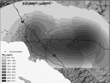
Figure 1 illustrates the pollution surface used in our main analysis, and the Appendix Figure (available with the
FIGURE 1.PM2.5exposure surface for Los Angeles interpolated with a hybrid universal–multiquartic model.
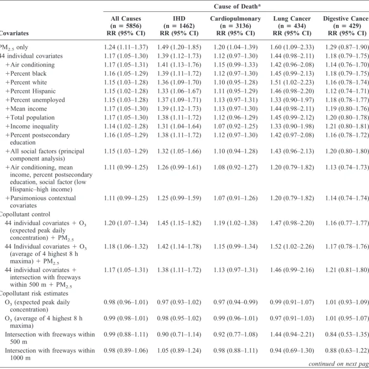
TABLE 1. Mortality Relative Risk Associated With a 10-g/m3Increase of PM
2.5Concentrations Based on 267 Zip Code Areas in Los Angeles in the American Cancer Society Cohort (1982–2000 follow up) for Various Causes of Death With Adjustment for Covariates Covariates Cause of Death* All Causes (nⴝ5856) RR (95% CI) IHD (nⴝ1462) RR (95% CI) Cardiopulmonary (nⴝ3136) RR (95% CI) Lung Cancer (nⴝ434) RR (95% CI) Digestive Cancer (nⴝ429) RR (95% CI) PM2.5only 1.24 (1.11–1.37) 1.49 (1.20–1.85) 1.20 (1.04–1.39) 1.60 (1.09–2.33) 1.29 (0.87–1.90) 44 individual covariates 1.17 (1.05–1.30) 1.39 (1.12–1.73) 1.12 (0.97–1.30) 1.44 (0.98–2.11) 1.18 (0.79–1.75) ⫹Air conditioning 1.17 (1.05–1.31) 1.41 (1.13–1.76) 1.15 (0.99–1.33) 1.42 (0.96–2.08) 1.14 (0.76–1.70) ⫹Percent black 1.16 (1.05–1.29) 1.39 (1.11–1.72) 1.12 (0.97–1.30) 1.45 (0.99–2.13) 1.18 (0.79–1.75) ⫹Percent white 1.15 (1.03–1.28) 1.36 (1.09–1.70) 1.10 (0.95–1.28) 1.51 (1.02–2.23) 1.16 (0.78–1.74) ⫹Percent Hispanic 1.15 (1.02–1.28) 1.33 (1.06–1.67) 1.11 (0.95–1.29) 1.46 (0.98–2.20) 1.12 (0.74–1.71) ⫹Percent unemployed 1.15 (1.03–1.28) 1.37 (1.09–1.71) 1.13 (0.97–1.31) 1.33 (0.90–1.97) 1.18 (0.78–1.77) ⫹Mean income 1.17 (1.05–1.30) 1.39 (1.12–1.73) 1.13 (0.97–1.30) 1.44 (0.98–2.11) 1.19 (0.80–1.76) ⫹Total population 1.17 (1.05–1.30) 1.38 (1.11–1.72) 1.12 (0.96–1.29) 1.45 (0.99–2.12) 1.20 (0.80–1.78) ⫹Income inequality 1.14 (1.02–1.28) 1.31 (1.04–1.64) 1.07 (0.92–1.25) 1.33 (0.90–1.98) 1.21 (0.80–1.81) ⫹Percent postsecondary education 1.16 (1.05–1.29) 1.38 (1.11–1.72) 1.12 (0.97–1.30) 1.42 (0.97–2.08) 1.16 (0.78–1.72)
⫹All social factors (principal component analysis)
1.15 (1.03–1.29) 1.32 (1.05–1.66) 1.10 (0.94–1.28) 1.43 (0.96–2.13) 1.20 (0.80–1.80)
⫹Air conditioning, mean income, percent postsecondary education, social factor (low Hispanic–high income) 1.11 (0.99–1.25) 1.26 (0.99–1.61) 1.08 (0.92–1.27) 1.20 (0.79–1.82) 1.13 (0.74–1.73) ⫹Parsimonious contextual covariates 1.11 (0.99–1.25) 1.25 (0.99–1.59) 1.07 (0.91–1.26) 1.20 (0.79–1.82) 1.14 (0.74–1.74) Copollutant control 44 individual covariates⫹O3
(expected peak daily concentration)⫹PM2.5 1.20 (1.07–1.34) 1.45 (1.15–1.82) 1.19 (1.02–1.38) 1.47 (0.98–2.20) 1.16 (0.77–1.77) 44 Individual covariates⫹O3 (average of 4 highest 8 h maxima)⫹PM2.5 1.18 (1.06–1.32) 1.42 (1.14–1.78) 1.15 (0.99–1.34) 1.52 (1.02–2.26) 1.17 (0.78–1.76) 44 individual covariates⫹ intersection with freeways within 500 m⫹PM2.5
1.17 (1.05–1.31) 1.38 (1.11–1.72) 1.13 (0.97–1.31) 1.46 (0.99–2.16) 1.21 (0.81–1.80)
Copollutant risk estimates O3(expected peak daily
concentration)
0.98 (0.96–1.01) 0.97 (0.93–1.02) 0.97 (0.94–0.99) 0.99 (0.91–1.07) 1.01 (0.93–1.09) O3(average of 4 highest 8 h
maxima)
0.99 (0.98–1.01) 0.98 (0.95–1.02) 0.99 (0.96–1.01) 0.97 (0.91–1.03) 1.01 (0.95–1.07) Intersection with freeways within
500 m
0.99 (0.88–1.11) 0.90 (0.71–1.14) 0.92 (0.77–1.08) 1.44 (0.94–2.21) 0.84 (0.53–1.35) Intersection with freeways within
1000 m
0.98 (0.89–1.06) 1.05 (0.89–1.24) 0.98 (0.88–1.11) 0.94 (0.69–1.30) 0.88 (0.63–1.22)
continued on next page
*ICD-9 code for ischemic heart disease (IHD) 410 – 414; for cardiopulmonary 400 – 440, 460 –519; for lung cancer 162; for digestive cancer 150 –159; for other cancers 140 –149, 160, 161, 163–239; for endocrine 240 –279; for diabetes 250; for digestive 520 –579; male accidents 800⫹; female accidents 800⫹.
online version of this article) illustrates the absolute and relative standard errors of estimation for the interpolated universal kriging surface. Approximately 50% of the mod-eled surface has errors that are less than 15% of the monitored value, whereas 67% of the surface lies within 20% of the
monitored values. For the most part, absolute standard errors for the densely populated areas of the study region are less than 3 g/m3. Only on the periphery of the study area do errors become large compared with monitored values, but these places have very few of our study subjects.
Interest-TABLE 1. Continued Cause of Death* Other Cancers (nⴝ992) RR (95% CI) Endocrine (nⴝ95) RR (95% CI) Diabetes (nⴝ57) RR (95% CI) Digestive (nⴝ151) RR (95% CI) Male Accidents (nⴝ75) RR (95% CI) Female Accidents (nⴝ47) RR (95% CI) All Others (nⴝ497) RR (95% CI) 1.09 (0.85–1.40) 3.22 (1.31–7.91) 2.38 (0.76–7.52) 2.17 (1.11–4.26) 1.52 (0.61–3.83) 1.08 (0.35–3.31) 1.11 (0.74–1.67) 1.06 (0.82–1.36) 2.75 (1.10–6.87) 2.10 (0.64–6.87) 1.98 (1.01–3.91) 1.35 (0.53–3.43) 0.86 (0.25–2.94) 1.13 (0.75–1.69) 1.06 (0.82–1.37) 2.73 (1.09–6.84) 2.10 (0.64–6.94) 1.95 (0.98–3.85) 1.50 (0.58–3.89) 1.01 (0.29–3.58) 1.05 (0.69–1.59) 1.05 (0.82–1.36) 2.70 (1.07–6.79) 2.09 (0.63–6.89) 2.02 (1.03–3.98) 1.29 (0.50–3.31) 0.91 (0.27–3.06) 1.10 (0.73–1.66) 1.05 (0.81–1.36) 2.55 (1.00–6.51) 2.05 (0.61–6.82) 1.96 (0.98–3.92) 1.19 (0.46–3.12) 0.93 (0.27–3.23) 1.10 (0.72–1.68) 1.04 (0.80–1.36) 2.60 (1.00–6.75) 2.07 (0.60–7.15) 1.72 (0.85–3.51) 1.41 (0.53–3.76) 0.71 (0.20–2.53) 1.17 (0.76–1.80) 1.01 (0.78–1.31) 2.27 (0.89–5.78) 1.82 (0.55–6.08) 1.83 (0.91–3.65) 1.51 (0.58–3.95) 0.88 (0.25–3.08) 1.10 (0.73–1.67) 1.07 (0.83–1.37) 2.61 (1.07–6.39) 2.06 (0.64–6.65) 1.99 (1.00–3.94) 1.35 (0.53–3.44) 0.80 (0.22–2.83) 1.12 (0.75–1.69) 1.06 (0.83–1.37) 2.76 (1.11–6.86) 2.10 (0.64–6.87) 2.02 (1.02–3.98) 1.35 (0.53–3.44) 0.72 (0.21–2.49) 1.12 (0.74–1.69) 1.08 (0.83–1.40) 2.84 (1.12–7.21) 2.15 (0.64–7.19) 1.98 (0.98–3.99) 1.29 (0.50–3.37) 0.74 (0.20–2.71) 1.15 (0.75–1.75) 1.05 (0.82–1.36) 2.72 (1.10–6.76) 2.07 (0.64–6.70) 1.99 (1.01–3.93) 1.41 (0.55–3.65) 0.89 (0.26–3.12) 1.14 (0.75–1.71) 1.06 (0.82–1.38) 2.50 (0.99–6.32) 2.12 (0.64–7.07) 1.88 (0.92–3.83) 1.17 (0.43–3.20) 0.59 (0.15–2.23) 1.21 (0.79–1.86) 1.04 (0.79–1.38) 2.40 (0.92–6.27) 1.92 (0.55–6.73) 1.55 (0.74–3.26) 1.89 (0.66–5.40) 0.64 (0.15–2.79) 1.11 (0.72–1.72) 1.06 (0.80–1.40) 2.29 (0.88–5.95) 1.79 (0.52–6.21) 1.55 (0.74–3.24) 1.88 (0.66–5.36) 0.70 (0.17–2.86) 1.10 (0.72–1.70) 1.08 (0.83–1.41) 2.59 (1.01–6.63) 2.17 (0.63–7.40) 1.91 (0.94–3.89) 1.35 (0.50–3.61) 1.12 (0.30–4.21) 0.95 (0.64–1.39) 1.07 (0.83–1.39) 2.76 (1.08–7.00) 2.29 (0.68–7.70) 1.82 (0.90–3.67) 1.29 (0.49–3.40) 0.98 (0.28–3.48) 0.98 (0.67–1.43) 1.08 (0.83–1.39) 2.49 (0.98–6.32) 1.82 (0.55–6.02) 2.20 (1.11–4.37) 1.34 (0.53–3.43) 0.73 (0.21–2.54) 1.02 (0.71–1.48) 0.99 (0.94–1.04) 1.05 (0.88–1.24) 0.98 (0.79–1.22) 1.02 (0.90–1.17) 1.00 (0.83–1.21) 0.87 (0.68–1.12) 1.06 (0.99–1.14) 0.99 (0.95–1.03) 1.00 (0.88–1.14) 0.94 (0.79–1.12) 1.06 (0.95–1.17) 1.03 (0.88–1.20) 0.93 (0.77–1.13) 1.04 (0.99–1.10) 1.19 (0.89–1.59) 0.64 (0.26–1.62) 0.45 (0.12–1.70) 2.54 (1.10–5.85) 0.57 (0.17–1.91) 0.87 (0.28–2.70) 0.87 (0.58–1.29) 0.90 (0.72–1.12) 1.55 (0.88–2.75) 1.77 (0.83–3.76) 0.49 (0.24–0.98) 1.05 (0.51–2.15) 2.02 (0.89–4.60) 1.15 (0.87–1.53)
ingly, the range of exposure within LA (20 g/m3) exceeds what we observed in previous studies based on contrasts among 116 cities (16g/m3).4
Results for all-cause and cause-specific deaths are re-ported in Table 1. This table shows the PM2.5 effect with
varying levels of control for confounding. Relative risks (RRs) are expressed as 10g/m3exposure contrasts in PM2.5
followed by the 95% confidence interval (95% CI). Using the example of all-cause mortality and with each succeeding stage, including the previous individual-level controls, we find that for PM2.5alone and controlling just for age, sex, and
race, the RR is 1.24 (95% CI⫽1.11–1.37), whereas the RR with the 44 individual confounders4is 1.17 (1.05–1.30). All subsequent results include the 44 individual-level control variables and one or more ecologic variables. For example, with 44 individual variables and the ecologic variable of unemployment, the RR of PM2.5is 1.15 (1.03–1.28). When
we add 4 social factors extracted from the principal compo-nent analysis (and accounting for 81% of the total variance in the social variables), the RR is 1.15 (1.03–1.29). Including all ecologic variables associated with mortality in bivariate mod-els reduces the pollution coefficient to RR of 1.11 (0.99 – 1.25). Finally, for the parsimonious model that includes ecologic confounder variables that both reduce the pollution coefficient and have associations with mortality, the RR is 1.11 (0.99 –1.25).
Comparing these results directly with the earlier anal-yses using between-community contrasts, the health effects are nearly 3 times greater for this analysis (ie, 17% increase compared with 6% in earlier studies in models that control for the 44 individual confounders). With control for neighbor-hood confounders, effect estimates are still approximately 50% to 90% higher than in previous analyses.
In models with only individual covariates and PM2.5,
some residual spatial autocorrelation was present in the ran-dom effects from the model clustered on zip code area. We attempted to remove this autocorrelation by fitting a model with aautocorrelation term that used mortality information from nearest neighbors as a predictor of mortality in the ZCAj,but the autocorrelation persisted (results not shown). When contextual socioeconomic status variables were in-cluded in the model, however, the Moran’sItests revealed no significant spatial autocorrelation. Table 2 shows the results of the Moran’sItest for all-cause and ischemic heart disease mortality. Visual inspection of the random effects, j,
con-firmed the results from the Moran’sItesting.
Sensitivity analyses using weighted estimation with weights equal to the inverse of the standard error on the universal kriging exposure model demonstrated that the risk estimates were robust to measurement error in the exposure estimate (results not shown). Point estimates remained elevated.
DISCUSSION
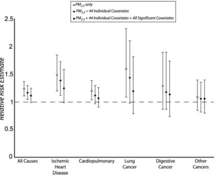
Our results suggest that the chronic health effects as-sociated with intraurban gradients in exposure to PM2.5may
be even larger than previously reported associations across metropolitan areas. Using the direct comparison to previous ACS studies, we see effects that are nearly 3 times larger than in models relying on between-community exposure contrasts. We also note convincing evidence of specificity in these health effects, with a stronger association between air pollu-tion and ischemic heart disease than for the more general measures of cardiopulmonary deaths or all-cause mortality (Fig. 2 displays the ordering in the risks presented in the tables). These findings concur with recent studies at the
TABLE 2. Results of the Spatial Autocorrelation Analysis on the Random Effects With Various Levels of Control for Confounding Model PM Effect RR (95% CI) Sigma Squared First-Order Neighborhood Matrix Second-Order Neighborhood Matrix Spatial Autocorrelation Moran’s I Normal PValue Spatial Autocorrelation Moran’s I Normal PValue All-cause mortality 44 individual covariates — 0.00701 0.078 0.021 0.038 0.812 PM2.5⫹44 individual covariates 1.165 (1.027–1.321) 0.00442 0.073 0.030 0.030 0.157 PM2.5⫹44 individual covariates⫹
parsimonious contextual covariates
1.120 (0.996–1.260) 0.00050 0.016 0.571 ⫺0.017 0.572
IHD mortality
44 individual covariates — 0.00476 0.025 0.419 0.037 0.154
PM2.5⫹44 individual covariates 1.391 (1.120–1.726) 0.00182 0.008 0.735 0.017 0.382
PM2.5⫹44 individual covariates⫹
parsimonious contextual covariates
metropolitan level, which again demonstrate that ischemic heart disease drives the cardiopulmonary association with air pollution.5
Among the cancer deaths, we also observe ordering in the risks, with decreasing risks as we move from lung cancer to digestive cancer to all cancers. Given that the lung would be most directly affected by air pollution, this finding gives corroborative evidence that the association did not occur by chance.
The larger effects in LA raise the question of whether some underlying aspect of this subcohort differs in charac-teristics that modify the association between mortality and air pollution. We compared the full cohort with the LA subco-hort and found no major differences in attributes likely to modify the air pollution–mortality association, with the ex-ception that the LA cohort was better educated. Based on the findings from the earlier analyses in which subjects with lower education experienced larger health effects,1,2,4we would expect the effect size in LA to be smaller than in the full cohort. Thus, differences in underlying characteristics appear unlikely to ex-plain the larger effects we observed in LA.
In comparing our results with the earlier national-level ACS studies, we examined the reduction in PM2.5levels in
LA to 50 other metropolitan areas that had data for 1980 and for the year 2000 we used in our study. (See Krewski et al2 for a description of the data.) The mean reduction was 31%, with a range from 0.4% to 59%. LA experienced a reduction of 24.5%, just above the lowest quartile of 23.5%. PM2.5has
therefore declined at a slightly slower rate in LA compared with much of the United States. If we assume that current PM2.5in LA is at 75.5% (ie, accounting for 24.5% reduction)
of the 1980 value and the average metropolitan area is at 69% of the 1980 value, some of the increase in the risks may be attributable to the relatively smaller reductions in LA. We tested this scaling effect by computing the ratio of reductions (0.69/75.5 ⫽ 0.914) and multiplied our raw coefficients by this factor before estimating the RR. The RR declines for all-cause mortality with the 44 individual variables to just over 15% and with maximal adjustment for confounders to 10%. Although reduced by up to 1.6%, we conclude that the majority of the increase over previous estimates reported by Pope et al34is probably not attributable to relative differences in the rate of reduction in ambient air pollution.
The findings for endocrine deaths also reveal another interesting possibility. Chronic air pollution exposure, similar to acute exposures,34 may adversely affect people with dia-betes more than the general population. Alternatively, the finding may indicate some uncontrolled confounding because we expect people with type 2 diabetes to live in neighbor-hoods with poorer social environments. This possibility ap-pears unlikely because of the extensive control we applied for contextual neighborhood variables. This potential problem appears improbable because we see internal validity in the effects of social confounders measured in the zip code areas. Although the accidental deaths were unexpectedly ele-vated in men, subsequent analyses revealed that the risks were attributable to deaths in the early years of the cohort before causes of death were coded in detail. As a result, we were unable to assess specific causes for this elevation.
Ozone had few elevated risks in any of our analyses and did not confound the relationship between particles and mortality. This finding agrees with earlier ACS studies
indi-FIGURE 2. Risk plots summarizing mortality relative risks (RR) and 95% CIs associated with a 10-g/m3 increase in ambient PM2.5by cause of death.
cating that ozone is not associated with elevated mortality risk,2,4 but contradicts studies on nonsmoking Adventists in southern California, where associations between lung cancer in males and ozone exposure were detected.35Recent national studies have reported elevated acute risks of ozone expo-sure,30but risk estimates were small, as would be expected of a study on acute as compared with chronic effects.36
In assessing the association with freeway buffers, point estimates were particularly elevated for lung cancer, endo-crine, and digestive mortality. The PM—mortality associa-tion remained robust to the freeway buffer, and risk estimates were unchanged when this variable was included in the model. Although imprecision in the freeway exposures re-sulting from the zip code area assignment of proximity may have biased our results toward the null, we did observe a RR for lung cancer of 1.44, and the other cause-specific mortality metrics indicate that more precise estimation of traffic effects are warranted in future research.
In previous studies based on the ACS cohort, all indi-viduals within the same metropolitan area were assigned the same level of exposure based on the average ambient con-centration observed at fixed-site air pollution monitors in that city. We hypothesized that the use of such a broad ecologic indicator of exposure leads to exposure measurement error, which in turn can bias estimates of mortality associated with air pollution exposure. Mallick et al37 analyzed the effect of this source of exposure measurement error based on plausible assumptions about error magnitude in the Six-Cities Study of air pollution and mortality.6This investigation suggested that the RR of mortality resulting from particulate air pollution may be underestimated by a factor of approximately 2- to 3-fold as a consequence of exposure misclassification, a finding consistent with the present results.
We recognize the possibility of exposure measurement error from using recent exposure models for a cohort enrolled in 1982. There are empiric as well as theoretical reasons that prevent this potential problem from seriously limiting the results. Empirically, other ACS analyses done at the metro-politan scale have found that these more recent exposure estimates predicted mortality with results similar to those based on earlier monitoring data.4 Also, the well-known meteorologic and topographic conditions of LA, along with a dominant on-shore breeze and steep mountains to the north and east, control much of the spatial pattern of pollution in the region. Our results agree with findings of earlier studies on the pattern of spatial variation in PM.38 Although levels may rise and fall in absolute terms, major changes in the spatial patterns within the region over time appear unlikely, and the rank ordering among assigned exposures should be maintained.
From a theoretical perspective, even if spatially heter-ogeneous changes to pollution levels within a city occurred as a result of new emissions during the follow up, this would
lead to larger exposure measurement error, and a bias toward the null would dominate, assuming a classic error structure. With a Berkson error structure, the variance of the dose– response estimate would be inflated.17 In either case, with current exposure models, the health effects likely have a lower probability of false-positive error, and we would expect the measurement error to reduce effect sizes and inflate their variance. High dose–response relationships can be caused by underestimation of concentrations in the high-exposure areas, but for these areas, the monitoring networks tend to be dense and the kriging errors were smaller than in most of the study area. Finally, the findings were robust to weighting for errors in the kriging estimate (ie, eastern parts of the LA region), which decreases the likelihood that elevated risks arise as a result of underestimation in the high-exposure groups.
Although we are unable to reconstruct likely exposures to PM2.5 for our exposure surface, we have assessed the
relationship at 51 central monitors between PM2.5measured
in 1980 and those of a period similar to that of our 2000 estimates (ie, 1999 –2000). These data were used in previous national studies,4 in which details on their derivation are available. Figure 3 illustrates the regression scatterplot for the 1999 –2000 values on the 1980 measurements. The coeffi-cient of determination is approximately 61%, and overall the latter periods are predicted well by the earlier measurements. In addition, we examined the relationship of historical PM10data in the LA area with the 2000 PM2.5estimates used
in our analysis. The period of maximal overlap between the sites occurs in 1993, where we had 8 PM10 readings at the
same locations as the subsequent PM2.5 measurements. By
FIGURE 3. 2000 PM2.5regressed onto 1980 PM2.5 (n⫽ 51 cities, R2⫽0.61).
regressing the 2000 PM2.5measurements on those PM10
mea-surements in 1993, we observe anR2value of 90% (Fig. 4). In both of these correlation analyses comparing earlier monitoring data with more recent PM2.5measurements, we
found evidence that areas with higher particle concentrations in earlier periods were likely to retain their spatial ranking. Those metropolitan areas likely to be high in 1980 also had a similar tendency in 2000.
Only the Norwegian cohort study has used time win-dows of exposure.39 In this study, the authors found that timing of the exposure window had little influence on the estimation of health effects; they used exposure windows in the middle of the follow-up period for most of their results. All of the other cohort studies have taken a similar approach to ours and computed the risk based on relatively short-term air pollution monitoring data. A case– control study in Stock-holm, Sweden, investigated time windows for lung cancer.40 This study found that windows of exposure 20 years before disease onset were more strongly associated with cancer than later periods. In our study, we found elevated risks of lung and digestive cancers, even with the more recent exposure model. The likely stability in the spatial pattern of exposure in LA probably accounts for this similarity of our findings to the 2 European studies that have used time windows.
Generally, our results agree with recent evidence sug-gesting that intraurban exposure gradients may be associated with even larger health effects than reported in interurban studies. Hoek et al8reported a doubling of cardiopulmonary mortality (RR⫽1.95; 95% CI 1.09 –3.52) for Dutch subjects living near major roads. Canadian cohort studies controlling for medical care utilization and preexisting chronic condi-tions through record linkage have also uncovered large health
effects with proximity to major roads at the intraurban scale.16 Recent results from the cohort in Norway also sug-gest associations between intraurban gradients in gaseous pollutants and mortality.40 All of these studies have impli-cated traffic as the source of pollution associated with the larger observed effects. In LA, the proportion of primary particles attributable to traffic is approximately 3.7%, whereas in the rest of the country, it is 0.75%.41Thus, beyond improved precision in the exposure models, the larger health effects reported here may be partly the result of higher proportions of traffic particulate in LA.
No previous studies have assessed associations based on a continuous exposure model with PM2.5, which limits the
use of the estimates for current policy debates that tend to focus on fine particles. In this study, we used PM2.5with a
continuous exposure metric that promotes comparison with previous studies on health effects and contributes to current regulatory debates.
REFERENCES
1. Pope CA, Thun MJ, Namboodiri MM, et al. Particulate air pollution as a predictor of mortality in a prospective study of US adults.Am J Respir Crit Care Med. 1995;151:69 – 674.
2. Krewski D, Burnet RR, Goldberg MS, et al.Reanalysis of the Harvard Six Cities and the American Cancer Society Study of Particulate Air Pollution and Mortality, Phase II: Sensitivity Analysis.Cambridge, MA: Health Effects Institute; 2000.
3. Jerrett M, Burnett R, Willis A, et al. Spatial analysis of the air pollution-mortality association in the context of ecologic confounders.J Toxicol Environ Health. 2003;66:1735–1777.
4. Pope CA, Burnett RT, Thun MJ, et al. Lung cancer, cardiopulmonary mortality, and long-term exposure to fine particulate air pollution. JAMA. 2002;287:1132–1141.
5. Pope CA, Burnett RT, Thurston GD, et al. Cardiovascular mortality and long-term exposure to particulate air pollution.Circulation. 2004;109: 71–77.
6. Dockery D, Pope CA3rd, Xu X, et al. An association between air pollution and mortality in six US cities.N Engl J Med. 1993;329:1753– 1759.
7. WHO Strategy on Air Quality and Health. Geneva: World Health Organization; 2001.
8. Hoek G, Brunekreef B, Goldbohm S, et al. Association between mor-tality and indicators of traffic-related air pollution in The Netherlands: a cohort study.Lancet. 2002;360:1203–1209.
9. Peters A, Pope CA. Cardiopulmonary mortality and air pollution. Lan-cet. 2002;360:1184 –1185.
10. Briggs D, de Hoogh C, Gulliver J, et al. A regression-based method for mapping traffic-related air pollution: application and testing in four contrasting urban environments.Sci Total Environ. 2000;253:151–167. 11. Zhu Y, Hinds W, Kim S, et al. Study of ultrafine particulates near a major highway with heavy-duty diesel traffic.Atmos Environ. 2002;36: 4323– 4335.
12. Jerrett M, Burnett RT, Kanaroglou P, et al. A GIS-environmental justice analysis of particulate air pollution in Hamilton, Canada.Environment and Planning.2001;A33:955–973.
13. Brauer M, Hoek G, van Vliet P, et al. Estimating long-term average particulate air pollution concentrations: application of traffic indicators and geographic information systems.Epidemiology. 2003;14:228 –239. 14. Brunekreef B, Holgate S. Air pollution and health.Lancet. 2002;360:
1233–1242.
15. O’Neill M, Jerrett M, Kawachi I, et al. Health, wealth and air pollution. Environ Health Perspect. 2003;111:186 –1870.
16. Finkelstein M, Jerrett M, DeLuca P, et al. A cohort study of income, air pollution and mortality.Can Med Assoc J. 2003;169:397– 402.
FIGURE 4.2000 PM2.5regressed onto 1993 PM10(n⫽8 sites in LA, R2⫽0.91).
17. Thomas DC, Stram D, Dwyer J. Exposure measurement error: influence on exposure— disease relationships and methods of correction. Annu Rev Public Health. 1993;14:69 –93.
18. Ku¨nzli N, McConnell R, Bates D, et al. Breathless in Los Angeles: the exhausting search for clean air. Am J Public Health. 2003;93:1494 – 1499.
19. Diez Roux AV. A glossary for multilevel analysis.J Epidemiol Com-munity Health.2002;56:588 –594.
20. Pickett KE, Pearl M. Multilevel analyses of neighbourhood socioeco-nomic context and health outcomes: a critical review. J Epidemiol Community Health. 2001;55:111–122.
21. Curtis S, Taket A.Health and Societies: Changing Perspectives. Lon-don: Edward Arnold; 1996.
22. Macintyre S, Ellaway A. Ecological approaches: rediscovering the role of the physical and social environments. In: Berkman L, Kawachi I, eds. Social Epidemiology. Oxford: Oxford University Press; 2000. 23. Evans GW, Kantrowitz E. Socioeconomic status and health: the
poten-tial role of environmental risk exposure. Annu Rev Public Health. 2002;23:303–331.
24. Willis A, Krewski D, Jerrett M, et al. Selection of ecologic covariates in the American Cancer Society study.J Toxicol Environ Health. 2003;66: 1591–1604.
25. Janssen N, Harssema H, Brunekreef B, et al. Assessment of exposure to traffic related air pollution of children attending schools near motorways. Atmos Environ. 2001;35:3875–3884.
26. Meng Q, Turpin B, Korn L, et al. Influence of ambient (outdoor) sources on residential indoor and personal PM2.5 concentrations: analyses of
RIOPA data.J Expo Anal Environ Epidemiol. 2005;15:17–28. 27. Luginaah I, Jerrett M, Elliott S, et al. Health profiles of Hamilton:
characterizing neighbourhoods for health investigations. GeoJournal. 2001;53:135–147.
28. Krieger N, Chen JT, Waterman PD, et al. Geocoding and monitoring of US socioeconomic inequalities in mortality and cancer incidence: does the choice of area-based measure and geographic level matter? The public health disparities geocoding project.Am J Epidemiol. 2002;156: 471– 482.
29. Burrough PA, McDonnell RA.Principals of Geographical Information Systems.Oxford University Press; 1998.
30. Bell ML, McDermott A, Zeger SL, et al. Ozone and short-term mortality in 95 US urban communities, 1987–2000.JAMA. 2004;292:2372–2378. 31. First Edition TIGER/Line Technical Documentation: US Bureau of the
Census Feature Class Codes (CFCC); 2004.
32. Hosmer W, Lemeshow S.Applied Survival Analysis.New York: Wiley and Sons; 1999.
33. Ma R, Krewski D, Burnett RT. Random effects Cox models: a Poisson regression modelling approach.Biometrika. 2003;90:157–169. 34. Goldberg MS, Burnett R, Bailar JC III, et al. The association between
daily mortality and ambient air particle pollution in Montreal, Quebec. 2. Cause-specific mortality.Environ Res. 2001;86:26 –36.
35. Abbey DE, Nishino N, McDonnell WF, et al. Long-term inhalable particles and other air pollutants related to mortality in nonsmokers. Am J Respir Crit Care Med. 1999;159:373–382.
36. Ku¨nzli N, Medina S, Kaiser R, et al. Assessment of deaths attributable to air pollution: should we use risk estimates based on time series or on cohort studies?Am J Epidemiol. 2001;153:1050 –1055.
37. Mallick R, Fung F, Krewski D. Adjusting for measurement error in the Cox proportional hazards regression model.J Cancer Epidemiol Pre-vent. 2002;7:155–164.
38. Kim BM, Teffera S, Zeldin MD. Characterization of PM2.5and PM10in
the South Coast Air Basin of southern California: part 1—spatial variations.J Air Waste Manag Assoc. 2001;50:2034 –2044.
39. Nafstad P, Lund Håheim L, Wisløff T, et al. Urban air pollution and mortality in a cohort of Norwegian men. Environ Health Perspect. 2004;112:610 – 615.
40. Nyberg F, Gustavsson P, Jarup L, et al. Urban air pollution and lung cancer in Stockholm.Epidemiology. 2000;11:487– 495.
41. 1999 National Emission Inventory Documentation and Data—Final Version 3.0. (1999). US Environmental Protection Agency, Technology Transfer Network Clearinghouse for Inventories & Emissions Factors web site. Available at: http://www.epa.gov/ttn/chief/net/1999inventory. html. Accessed February 1, 2005.