Estimation and simulation in directional and statistical shape models

and Statistical Shape Models

Asaad Mohammed Ganeiber

Submitted in accordance with the requirements for the degree of Doctor of Philosophy

The University of Leeds

School of Mathematics

The candidate confirms that the work submitted is his own and that appropriate credit has been given where reference has been made to the work of others.

This copy has been supplied on the understanding that it is copyright material and that no quotation from the thesis may be published without proper acknowledgement.

Copyright c 2012 The University of Leedsand Asaad Mohammed Ganeiber

The right of Asaad Mohammed Ganeiber to be identified as Author of this work has been

Acknowledgements

First of all, praise be to Allah for the glory of Islam who told us in the Holy Koran “Verily, the noblest of you, in the sight of Allah, is the best in conduct and Allah has full knowledge and is well acquainted” [Koran XLIX:13].

Next, I offer my gratitude and sincere thanks to my supervisor Professor John T. Kent. He has taught me, both consciously and un-consciously, how good research study is done. I appreciate all his contributions of time and ideas to make my PhD experience productive and stimulating. The joy and enthusiasm he has for his research were contagious and motivational for me, even during tough times in the PhD pursuit. I am also thankful for the excellent example he has provided as a successful statistician and professor. I am also very grateful to the Senior Research Professor Kanti V. Mardia, Professor Ian L. Dryden, ProfessorCharles C. Taylor, SirDavid R. Cox, ProfessorDavid Firth, ProfessorSimon Wood, Pro-fessorFred Bookstein, ProfessorWilfrid Kendall, ProfessorChristian Klingenbergand Professor Andrew Wood for all the advanced background materials in Statistics I obtained during my attending some academic classes in the School of Mathematics, departmental seminars and conferences in UK. I would like also to take this opportunity to thank all those who have contributed in any way, shape or form to the completion of this thesis. I am grateful to Dr Robert G. Aykroyd and Dr Alfred Kumefor comments which helped to improve the clarity of the thesis, Dr Leonid V. Bogachev and the postgraduate secretary MrsJeanne S. Shuttleworthin School of Mathematics for their administrative advices and assistants, friends for their ideas and criticisms. My time in Leeds was made enjoyable in large part due to the many friends and groups that became a part of my life.

Lastly, I would like to thank my family for all their love and encouragement. For my parents and my brother Mr Ahmed M. Ganeiber who raised me with a love of science and supported me in all my pursuits. Without their assistance this work would not have been possible. Thank you.

This thesis is concerned with problems in two related areas of statistical shape analysis in two dimensional landmarks data and directional statistics in various sample spaces.

Directional observations can be regarded as points on the circumference of a circle of unit radius in two dimensions or on the surface of a sphere in three dimensions. Special directional methods and models are required which take into account the structure of these sample spaces. Shape analysis involves methods for the study of the shape of objects where location, scale and orientation are removed. Specifically, we consider the situation where the objects are summarized by points on the object called landmarks. The non-Euclidean nature of the shape space causes several problems when defining a distribution on it. Any distribution which could be considered needs to be tractable and a realistic model for landmark data. One aim of this thesis is to investigate the saddlepoint approximations for the normalizing constants of some directional and shape distributions. In particular, we consider the normalizing constant of the CBQ distribution which can be expressed as a one dimensional integral of normalizing constants for Bingham distributions. Two new methods are explored to evaluate this normalizing constant based on saddlepoint approximations namely the Integrated Saddlepoint (ISP) approximation and the Saddlepoint-Integration (SPI) approximation.

Another objective of this thesis is to develop new simulation methods for some directional and shape models. We propose an efficient acceptance-rejection simulation algorithm for the Bingham distribution on unit sphere using an angular central Gaussian (ACG) density as an envelope. This envelope is justified using inequalities based on concave functions. An immediate consequence is a method to simulate 3×3 matrix Fisher rotation matrices. In addition, a new accept-reject algorithm is developed to generate samples from the complex Bingham quartic (CBQ) distribution.

The last objective of this thesis is to develop a new moment method to estimate the parameters of the wrapped normal torus distribution based on the sample sine and cosine moments.

Contents

1 Introduction 1

1.1 Directional Statistics . . . 1

1.1.1 Circular Models . . . 2

1.1.2 Spherical Models . . . 3

1.1.3 Special Orthogonal Rotation Matrices and Torus Models . . . 4

1.2 Statistical Analysis of Shapes . . . 4

1.2.1 Shapes and Landmarks . . . 4

1.2.2 Configurations . . . 6

1.2.3 Shape and Pre-Shape Spaces . . . 6

1.2.4 Shape Models . . . 9

1.2.5 Relationship between Directional Statistics and Shape Analysis . . . 10

1.3 Outline of the Thesis . . . 11

1.3.1 Part I: Saddlepoint Approximations . . . 11

1.3.2 Part II: Rejection Simulation Techniques . . . 13

1.3.3 Part III: Methods of Estimation for Torus Data . . . 14

I

Saddlepoint Approximations

16

2.2 Background Ideas . . . 18

2.3 Simple Saddlepoint Approximations . . . 19 iii

2.4 Refined Saddlepoint Approximations and Motivation . . . 21

2.5 Tilting and Saddlepoint Approximations . . . 24

2.6 Noncentral Chi-square Distribution . . . 25

2.7 von Mises (Circular Normal) Distribution . . . 32

2.7.1 Background . . . 32

2.7.2 Saddlepoint Approximations for the Normalizing Constant . . . 35

2.7.3 Saddlepoint Approximations for the Mean Resultant Length . . . 36

2.8 Fisher Distribution on the Sphere . . . 39

2.8.1 Background . . . 39

2.8.2 Saddlepoint Approximations for the Normalizing Constant . . . 41

2.9 Bingham Distribution on the Sphere . . . 44

2.9.1 Background . . . 44

2.9.2 Saddlepoint Approximations for the Normalizing Constant . . . 47

3 Saddlepoint Approximations for the Complex Bingham Quartic Distribution 50 3.1 Introduction . . . 50

3.2 Quadrature Methods . . . 50

3.2.1 Trapezoidal Rule . . . 51

3.2.2 Recursive Adaptive Simpson Quadrature . . . 52

3.2.3 Gauss-Legendre Quadrature . . . 52

3.3 Saddlepoint Approximations for Finite Mixtures . . . 53

3.3.1 Background on Finite Mixtures . . . 53

3.3.2 Saddlepoint Approximations . . . 54

3.3.3 Application to Gamma Mixture Distribution . . . 55

3.4 Complex Bingham Quartic Distribution . . . 57

3.4.1 Background . . . 58

3.4.2 Decomposition of Quadratic Forms . . . 59

3.4.3 Some Properties and Motivation . . . 60

3.4.4 Representation of the Normalizing Constant . . . 61

3.4.5 Saddlepoint Approximations for the Normalizing Constant: Integrated Saddlepoint Approximations Approach . . . 62

CONTENTS v

3.4.6 Saddlepoint Approximations for the Normalizing Constant:

Saddlepoint of Integration Approximations Approach . . . 63

3.4.7 Change of Variables . . . 64

3.4.8 Performance Assessment for Mixture Saddlepoint Approximations Approaches 68

II

Rejection Simulation Techniques

76

4.2 Principles of Acceptance-Rejection Simulation Scheme . . . 78

4.3 Envelopes Based on Concave Functions . . . 80

4.4 Simulation from the Multivariate Normal Distribution with Multivariate Cauchy En-velope . . . 83

4.5 Bilateral Exponential Envelope for Standard Normal Distribution . . . 84

4.6 Simulation from the Real Bingham Distribution with ACG Envelope . . . 86

4.7 Simulation from the von Mises Distribution with a Wrapped Cauchy Envelope . . . 90

4.8 Link Between the Best-Fisher Method and the Concave Inequality . . . 92

4.9 Simulation from the Matrix Fisher Distribution . . . 95

4.9.1 The Matrix Fisher Probability Density Function . . . 95

4.9.2 Simulation Scheme . . . 95

5 General Techniques of Simulation from Directional and Shape Models 99 5.1 Introduction . . . 99

5.2 A Brief Historical Survey of Simulation Methods . . . 100

5.3 Simulation from the von Mises and von Mises-Fisher Distributions . . . 102

5.3.1 von Mises Distribution with Real Bingham Envelope . . . 102

5.3.2 von Mises-Fisher Distribution with Beta Envelope . . . 104

5.4 Bipartite Rejection Scheme for the Real Bingham Distribution on the Sphere . . . . 108

5.6 Simulation from the Fisher-Bingham (FB5) Distribution . . . 112

5.6.1 Background . . . 112

5.6.2 FB5 Distribution with Uniform Envelope . . . 113

5.6.3 FB5 Distribution with Truncated Exponential Envelope . . . 114

5.7 Simulation from the Complex Bingham Distribution . . . 116

5.7.1 The Complex Bingham Density Function . . . 116

5.7.2 Simulation Schemes . . . 118

5.8 Simulation from the Complex Bingham Quartic Distribution . . . 120

III

Methods of Estimation for Torus Data

127

6.2 Bivariate von Mises Torus Distribution . . . 129

6.2.1 Marginal and Conditional Models . . . 132

6.2.2 Comparing Models using Log-Densities . . . 133

6.3 Moments and Correlations Under High Concentration . . . 134

6.4 Approaches to Estimation . . . 140

6.4.1 Maximum Likelihood Method . . . 140

6.4.2 Maximum Pseudolikelihood Method . . . 141

6.5 Wrapped Normal Torus Distribution . . . 142

6.5.1 Overview and Background . . . 142

6.5.2 Moments for the Wrapped Normal Torus Distribution . . . 144

7 Conclusions and Future Directions 147 7.1 Saddlepoint Approximation . . . 147

7.1.1 Motivation . . . 147

7.1.2 Critical Summary . . . 147

7.1.3 Future Work . . . 148

7.2 Simulation Techniques . . . 148

CONTENTS vii

7.2.2 Critical Summary . . . 148

7.2.3 Future Work . . . 149

7.3 Estimation Methods for Torus Data . . . 149

7.3.1 Motivation . . . 149

7.3.2 Critical Summary . . . 149

7.3.3 Future Work . . . 150

A Appendix A 151 A.1 R Functions for Simulating Bingham Distribution using ACG Envelope . . . 151

A.2 R Functions for Best-Fisher algorithm of the von Mises Distribution . . . 153

A.3 MATLAB Functions for Simulating von Mises-Fisher Distribution . . . 154

A.4 Evaluate _E cosθ1sinθ2 = 0 for the Bivariate Sine Distribution . . . 163

1.1 Relationship between some common directional and shape distributions.. . . 15 2.1 Numerical unnormalizing first order saddlepoint approximations and unnormalizing second order

saddlepoint approximations for the normalizing constant of the von Mises distribution with various values of the concentration parameterκ. . . 37 2.2 Numerical unnormalizing first order saddlepoint approximations and unnormalizing second order

saddlepoint approximations for the mean resultant length of the von Mises distribution with various values of the concentration parameterκ. . . 39 2.3 Numerical first order saddlepoint approximations ˆc02 and second order saddlepoint approximations

ˆ

c03for the normalizing constant of the Fisher distribution under various values ofκ;nis the sample

size required for the difference between the trueκand ˆκ3to be significant at the level 5% level when

large sample likelihood ratio test is used (see Kume and Wood [54]). . . 45 2.4 Numerical results for the second order saddlepoint approximations for the normalizing constant of

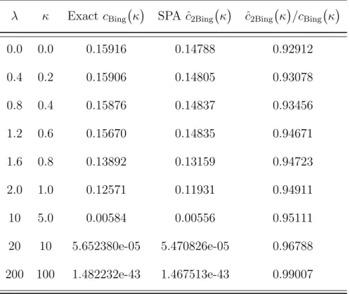
the real Bingham distribution with varyingκ. . . 49 3.1 Numerical results for true value of the normalizing constant of the complex Bingham quartic

distribu-tioncCBQ(Ω): The second order integrated saddlepoint ˆcCBQ,ISP(Ω) approximations and the second

order saddlepoint of integration ˆcCBQ, SPI(Ω) approximations with various values of κ, β = 0.4κ, λ1,λ2 andn= 1000. . . 74

3.2 Numerical results for the second order integrated saddlepoint ˆcCBQ,ISP(Ω) and the second order

saddlepoint of integration ˆcCBQ, SPI(Ω) approximations with/without change of variable, with λ1, λ2,λ3 andλ4 varying and withn= 1000. . . 75

LIST OF TABLES ix

4.1 Analytical efficiencies for Multivariate Normal/Multivariate Cauchy Envelope A/R simulation with various values ofpandb. . . 85 4.2 Simulated efficiencies rates and their standard errors for Bingham/Angular central Gaussian (ACG)

Envelope A/R simulation withn= 10000 and various values ofλ1,λ2andλ3= 0. . . 90

4.3 Simulated efficiencies rates and their standard errors for matrix Fisher/Angular central Gaussian (ACG) Envelope A/R simulation with n= 1000 and various values of φ1, φ2, φ3, λ1, λ2, λ3 and λ4= 0. . . 98

5.1 Analytical efficiencies for Von Mises/Wrapped Cauchy, Beta and Real Bingham Envelopes A/R simulation A/R simulation with various values ofκ,τ,ρandx0. . . 107

5.2 Analytical efficiencies for Bingham/Bipartite Envelopes A/R simulation with various values ofκ. . 110 5.3 Analytical efficiencies for the FB5 distribution based on the Kent-Hamelryck, the uniform and the

real Bingham envelopes A/R simulation with various values ofκandβ (κ >2β). . . 117 5.4 Simulated efficienciesM of truncated multivariate exponential envelope and angular central

Gaus-sian envelope needed for the simulation methods from the complex Bingham distribution with k

varying and with a common concentration valueλ. . . 121 5.5 Simulated efficiencies rates and their standard errors for the complex Bingham quartic (CBQ)

dis-tribution/Mixture Multivariate Normals and the Kent-Hamelryck envelopes in the casek= 3 with various values ofκ,β, λ1,λ2and a sample of sizen= 10000 (fixed 2β/κ <1). . . 125

5.6 Simulated efficiencies rates and their standard errors for the complex Bingham quartic (CBQ) dis-tribution/Mixture Multivariate Normals envelope in the casek = 4 with various values of λ1, λ2, λ3,λ4 and a sample of sizen= 1000. . . 126

6.1 Simulated moment estimations for the parameters of the wrapped bivariate normal torus distribution with a sample of sizen= 100. . . 146

1.1 Stereographic projection . . . 3

1.2 The hierarchies of the various spaces (after Goodall and Mardia [26]). . . 8

1.3 The hierarchies of some common shape and directional distributions. . . 12

2.1 The cumulant generating functionKS(u) for noncentral Chi-square distribution versusu. . . 27

2.2 Saddlepoint function ˆu(s) versuss . . . 28

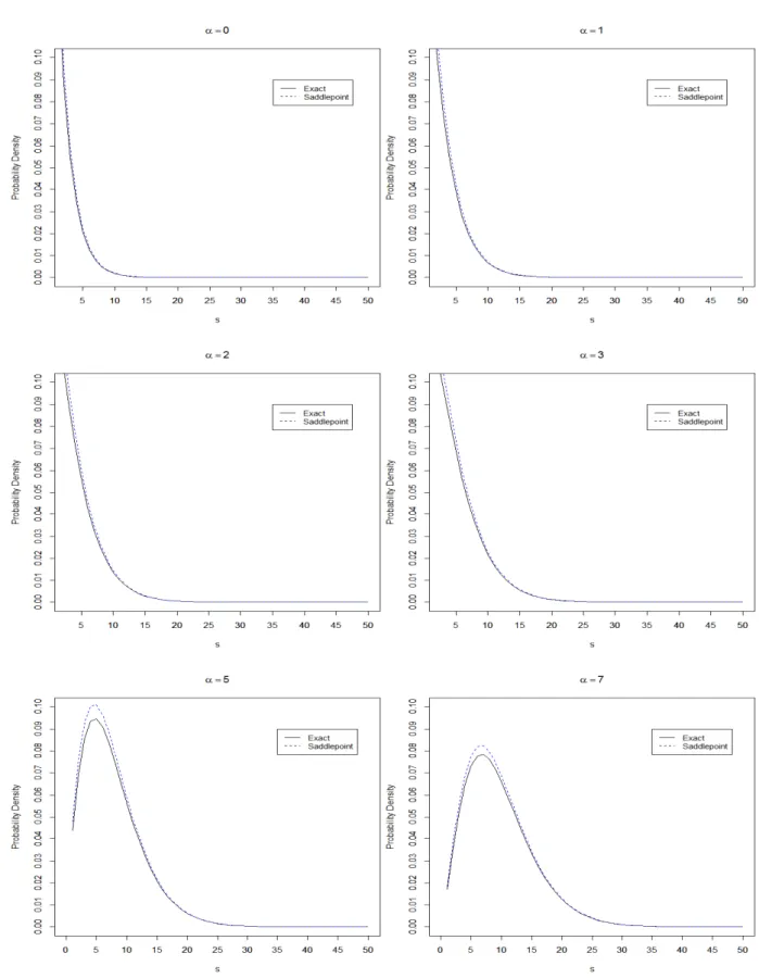
2.3 Exactf(s) (solid curve) and first-order saddlepoint density approximation ˆf1(s) (dashed line) versus s for noncentral chi-square distribution with various values of the noncentrality parameter α = 0,1,2,3,5 and 7.. . . 30

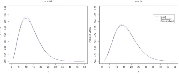
2.4 Exactf(s) (solid curve), unnormalized first-order saddlepoint density approximation ˆf1(s) (dashed curve) and the normalized first-order saddlepoint density approximation ¯f(s) (dotted curve) versus sfor noncentral chi-square distribution. . . 32

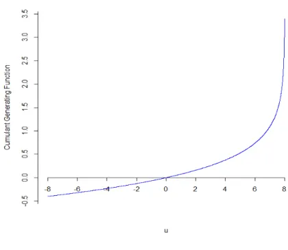
3.1 The cumulant generating functionK(u) for the gamma mixture versusu. . . 56

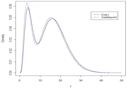
3.2 Gamma mixture random variable: Exact density and saddlepoint approximation. . . 57

3.3 The functionh Ψ(s) versus s. . . 67

3.4 The cumulant generating functionKR2(u) versusu. . . 69

3.5 The saddlepoint approximation for the real Bingham distribution ˆcBing Ψ(s)versuss.. . . 71

3.6 The ratio ˆcCBQ(Ω)/cCBQ(Ω) against the concentration parameterκ.. . . 73

4.1 The concave function ϕ(u) and the linear function ψ(u) versus u. In the left panel b = 15 and q= 10. In the right panelb= 10,q= 30 andu0= 10. . . 81

LIST OF FIGURES xi

4.2 The unnormalized standard normal functionf∗(x) and the unnormalized bilateral envelope function

g∗(x) versusx. In the left panelα= 0.3 whereas in the right panel α= 1.0. . . 85 4.3 The von Mises functionf(θ) and the the simulation proportional envelope of the wrapped Cauchy

distributionM gΘ(θ). In the left panelκ= 1.0,τ= 3.236,ρ= 0.346 and M = 1.152 whereas in the

right panelκ= 10,τ = 21.02,ρ= 0.727 andM = 1.481. . . 92 5.1 Envelope rejection for the von Mises functionf(θ) with Bingham target distributiong(θ) forκ= 5.0

andM = 1.20. . . 104 5.2 Spherical plot of two random samples with 200-points each from von Mises-Fisher distribution

aroundµ= [1 0 0] andκ= 2,10 from left to right, respectively. . . 108 6.1 Contour plots of log-densities (normalizing constant omitted) for the sine, cosine with positive

in-teraction and cosine with negative inin-teraction models. Captions indicate the vector of parameters:

κ1, κ2, η (Positive) for the sine model,κ1, κ2, γ1 (Positive) for the cosine model with positive

inter-action model andκ1, κ2, γ2 (Positive) for cosine with negative interaction models. . . 135

6.2 Contour plots of log-densities (normalizing constant omitted) for the sine, cosine with positive interaction and cosine with negative interaction models. Captions indicate the vector of parameters:

κ1, κ2, η (Negative) for the sine model, κ1, κ2, γ1 (Negative) for the cosine model with positive

interaction model andκ1, κ2, γ2 (Negative) for cosine with negative interaction models. . . 136

6.3 3D perspective plots of the log-densities (normalizing constant omitted) for the sine, cosine with positive interaction and cosine with negative interaction models. Captions indicate the vector of parameters: κ1, κ2, η (Positive) for the sine model, κ1, κ2, γ1 (Positive) for the cosine model with

positive interaction model andκ1, κ2, γ2 (Positive) for cosine with negative interaction models. . . 137

6.4 3D perspective plots of the log-densities (normalizing constant omitted) for the sine, cosine with positive interaction and cosine with negative interaction models. Captions indicate the vector of parameters: κ1, κ2, η (Positive) for the sine model, κ1, κ2, γ1 (Positive) for the cosine model with

positive interaction model andκ1, κ2, γ2 (Positive) for cosine with negative interaction models. . . 138

6.5 Simulated bivariate normal torus data with small varianceσ2_{= 1.0 and strong correlationρ= 0.90}

for a sample of sizen= 100. (a) before wrapping; (b) after wrapping. . . 143 6.6 Simulated bivariate normal torus data with large varianceσ2_{= 50 and strong correlationρ= 0.90}

6.7 Simulated bivariate normal torus data with large varianceσ2 = 50 and weak correlation ρ= 0.50 for a sample of sizen= 100. (a) before wrapping; (b) after wrapping. . . 144

Chapter

1

Introduction

The work contained in this thesis falls into the two related areas of statistical shape analysis and directional statistics. Let us start by introducing the fields involved in this thesis. Basic definitions referred to through out the text are given.

1.1

Directional Statistics

There are various statistical problems which arise in the analysis of data when the observations are directions. Directional data are often met in astronomy, biology, geology, medicine and meteorol-ogy, such as in investigating the origins of comets, solving bird navigational problems, interpreting palaeomagnetic currents, assessing variation in the onset of leukaemia, analysing wind directions, etc.

The directions are regarded as points on the circumference of a circle in two dimensions or on the surface of a sphere in three dimensions. In general, directions may be imagined as points on the surface of a hypersphere but observed directions are obviously angular measurements.

The difficulty in the statistical analysis of directional data stems from the disparate topology of the circle and the straight line: if angles are recorded in radians in the range [−π, π), then directions close to the opposite end-points are near neighbours in a metric which respects the topology of the circle, but maximally distant in a linear metric. Thus, many standard statistical procedures are inappropriate for modelling directional data (Coles [10]).

1.1.1

Circular Models

A large number of circular probability models exists; like linear probability models, they may be either discrete or continuous. Several of the more important are discussed in this thesis.

Many useful and interesting circular models may be generated from probability distributions on the real line or on the plane, by a variety of mechanisms. We describe a few such general methods (Jammalamadaka and SenGupta [31], p. 30):

(1) By wrapping a linear distribution around the unit circle. Any linear random variable X on the real line may be transformed to a circular random variable by reducing it modulo 2π i.e. using θ = X(mod 2π). The wrapped normal and the wrapped Cauchy distributions are of interest in this thesis.

(2) Through characterizing properties such as maximum entropy, etc. It is often instructive to ask if there are distributions on the circle which enjoy certain desirable properties. For in-stance, one may ask which distribution has the maximum entropy subject to having non-zero trigonometric moments. The uniform and von Mises (Circular Normal) distributions have the maximum entropy (Mardia and Jupp [70]. p. 42) where the entropy of a distribution on the circle with probability density function f is defined as

H(f) =−

Z 2π

0

f(θ) logf(θ)d θ.

This is one way of measuring the closeness of a distribution to the uniform distribution. von Mises distribution is of interest in this thesis. Moreover, if we ask which distribution on the circle has the property that the sample mean direction and the length of the resultant vector are independent, then the uniform or isotropic distribution is the answer (see Kent et. al. [47] and Jammalamadaka and SenGupta [31], p. 32). This characterization of the uniform distribution is similar to, and as important as, that of the normal distribution on the line as the only one in which the sample mean and sample variance are independent.

(3) By transforming a bivariate linear random variable to just its directional component, the so-called offset distributions. This is done by accumulating probabilities over all different lengths for a given direction. We transform the bivariate random vector (X, Y) into polar co-ordinates (r, θ) and integrate overr for a given θ. If f(x, y) denotes the joint distribution of a bivariate

1.1. DIRECTIONAL STATISTICS 3

distribution on the plane, then the resulting circular offset distribution, say g(θ), is given by

g(θ) =

Z ∞

0

f(rcosθ, rsinθ)rd r.

(4) One may start with a distribution on the real line, and apply a stereographic projection that identifies points xwith those on the circumference of the circle, sayθ. This correspondence is one-to-one except for the fact that the mass if any, at both +∞and−∞, are identified withπ

(Jammalamadaka and SenGupta [31], p. 31). Such a correspondence is shown in Figure 1.1.

Figure 1.1: Stereographic projection

1.1.2

Spherical Models

Much of the theory of spherical statistics is analogous to that for circular statistics. Further, one can consider directions inpdimensions, i.e. unit vectors inp-dimensional Euclidean space_Rp. Directions in p dimensions can be represented as unit vectors x, i.e. as points on Sp−1 _{= x: x}T_{x= 1}

, the (p−1)-dimensional sphere with unit radius and centre at the origin. Some spherical distributions are of interest in this thesis namely, von Mises-Fisher, Fisher, Fisher-Bingham (Kent) distributions for the spherical data and the Bingham and the angular central Gaussian (ACG) distributions for the axial data.

1.1.3

Special Orthogonal Rotation Matrices and Torus Models

In the previous subsections we have considered mainly observations which are unit vectors (di-rections) or axes. However, other types of observations occur in directional statistics, the most important of these from the practical point of view being rotations, orthonormal frames and torus.

An orthonormal r-frame in _Rp _{is a set (x}

1,x2, . . . ,xp) of orthonormal vectors in Rp. The space

of orthonormal r-frame in _Rp is called the Stiefel manifold Vr(Rp). In terms of p ×r matrices

X, Vr(Rp) =

X : XTX = Ir . An orthonormal p-frame is equivalent to an orthogonal matrix,

so Vr(Rp) = O(p), the orthogonal group consisting of all orthogonal p×p matrices. Moreover, an orthogonal (p−1)-frame (x1,x2, . . . ,xp−1) can be extended uniquely to an orthogonal p-frame

(x1,x2, . . . ,xp) with matrix of determinant 1, so Vr(Rp) = SO(p), the special orthogonal group consisting of all p × p rotation matrices (Mardia and Jupp [70], p. 285). The matrix Fisher distribution on a group SO(3) of all rotations of _R3 is of interest in the simulation chapters in this thesis.

In geometry, a torus is a surface of revolution generated by revolving a circle in three dimensional space about an axis coplanar (all the points lie in the same geometric plane) with the circle. In topology, a torus is homeomorphic to the Cartesian product of two circles: _T2 =S1×S1 (Nikulin and Shafarevich [78], p. 110). Sometimes it is necessary to consider the joint distribution of two circular random variable θ1 and θ2. Then (θ1, θ2) take values on the unit torus. In the uniform

distribution on the torus, θ1 and θ2 are independent and uniformly distributed. Some interested

distributions on the torus are the bivariate von Mises (sine and cosine) distribution and the wrapped multivariate normal distribution.

1.2

Statistical Analysis of Shapes

1.2.1

Shapes and Landmarks

Shape is all the geometrical information that remains when location, scale and rotational effects are filtered out from an object.

According to this, definition of shape is invariant under Euclidean similarity transformations of translation, scaling and rotation as follows. The simplest type of object which can be studied consists of a labelled set of k points in _Rm (where k ≥m = 1), represented as a k×m matrix, X,

1.2. STATISTICAL ANALYSIS OF SHAPES 5

say. Then for any location vectorγ ∈_Rm_{, orthogonalm×mrotation matrix Γ satisfying det(Γ) = 1}

and ΓT_{Γ = ΓΓ}T _=I

m, and a scaleβ >0,Xhas the same shape asβXΓ+1kγT (Euclidean similarity

transformation of X). Similarity transformations in _R2 can also use complex notation. Consider

k ≥3 landmarks in _C, zo _{= (z}o

1, z2o, . . . , zok)T which are not all coincident. The Euclidean similarity

transformations of zo are βeiθzo+ 1kξ where β ∈ R+ is the scale, 0≤θ < 2π is the rotation angle and ξ ∈_Cis the translation.

A related concept to shape is form. It is the geometrical information that remains when location and rotational effects are filtered out from an object. In other words two objects have the same size-and-shape (form) if they can be translated and rotated to each other so that they match exactly, i.e if the objects are rigid body transformations of each other.

The next question that naturally arises is: How should one describe a shape? One way to describe a shape is by locating a finite number of points on the outline. Consequently, the concept of a landmark is adopted by Dryden and Mardia [18].

A landmark is a point in two or three-dimensional space that corresponds to the position of a particular feature on an object of interest. For example, in the study of osteological remains, a landmark might be defined as the point that marks the scar of a muscle insertion on a bone, the intersection of two or more bones at a cranial suture, or the foramen that marks the path of a neurovascular bundle. We choose to focus on landmark data because we want to analyze data for which points on one object have an unambiguous correspondence to points on another object (Lele and Richtsmeier [56], p. 14).

Dryden and Mardia [18] split landmarks into three subgroups:

1. Anatomical landmarks: Points assigned by an expert that correspond between organisms in some biologically meaningful way.

2. Mathematical landmarks: Points located on an object according to some mathematical or geometrical property, i.e. high curvature or an extremum point.

3. Pseudo-landmarks: Constructed points on an object either on the outline or between land-marks.

1.2.2

Configurations

A mathematical representation of ak-point shape in mdimensions could be created by concatenate each dimension into a km-vector. The vector representation x for planar shapes (m = 2) would then be:

x= [x1, x2, . . . , xk, y1, y2, . . . , yk]T.

Alternatively, we may recast a km-vector as a configuration matrix with k rows and m columns. Thus, the configuration matrix X for planar shapes (m = 2) would then be:

X =         x1 y1 x2 y2 .. . ... xk yk         .

To perform a shape analysis, a biologist traditionally selects ratios of the distances between landmarks or angles, and then submits these to a multivariate analysis. This approach has been called multivariate morphometrics or the traditional method. Another approach is to consider a shape space obtained directly from the landmark coordinates, which retains the geometry of a point configuration, this has been called geometric shape analysis or the geometrical method.

Shape variables are features constructed from the configuration X that are unchanged under similarity transformations (translation, scaling and rotation). Similarly size-and-shape or form variables are unchanged under rigid body motions (translation and rotation). Size variables are form variables that are invariant under scaling changes; that is, if β > 0 is some constant, the size variable for βX must beβ times the size variable for X.

1.2.3

Shape and Pre-Shape Spaces

Shape space is the set of all possible shapes. Formally, the shape space Σk_m is the orbit space of the non-coincident k point set configurations in _Rm _{under the action of the Euclidean similarity}

transformations.

The pre-shape, Z, of a configuration matrix X has all the information about location and scale removed. it is usually constructed by centring the configuration and then dividing by size. The

1.2. STATISTICAL ANALYSIS OF SHAPES 7

pre-shape is given by

Z= H X kH Xk

whereHis a (k−1)×kHelmert matrix without the first row and it is called the Helmert sub-matrix. The centred pre-shape,ZC =C X/kC Xkis another pre-shape representation whereC=Ik−1_k1k1Tk

is centred matrix and also an idempotent (CTC = C, C2 = C) (Dryden and Mardia [18], p.55). Note thatZ is a (k−1)×mmatrix whereas ZC is ak×mmatrix and the relationship between the

pre-shape and centred pre-shape isZC =HTZ. Both pre-shape representations are equally suitable

for the pre-shape space which has real dimension km−1. The advantage in using Z is that it is of full rank and its dimension is less than that of ZC. On the other hand, the advantage of working

with the centred pre-shapeZC is that a plot of the Cartesian coordinates gives a correct geometrical

view of the shape of the original configuration (Dryden and Mardia [18], p.55).

Pre-shape space is the space of all possible pre-shapes. Formally, the pre-shape space Sk

m is the

orbit space of the non-coincident k point set configurations in _Rm _{under the action of translation}

and isotropic scaling.

If we remove translation from the original configuration then the resulting landmarks are called Helmertized. Filtering scale from those Helmertized landmarks yields pre-shape whereas eliminating rotation from them should create size-and-shape. Again, removing rotation from pre-shape or removing scale from size-and-shape should result shape and after removing reflection for these shape landmarks the result is reflection shape (Dryden and Mardia [18], p.55). Figure 1.2 gives a diagram indicating the hierarchies of the different spaces.

Complex arithmetic when m = 2 enables us to deal with shape analysis very effectively. The advantage of using complex notation is that rescaling and rotation of an object in two dimensions can be obtained by complex multiplication by a complex number; for example, λz=rexp(i θ)zhas the same shape asz, although being rescaled by rand rotated anticlockwise by θ radians about the origin (Mardia [63]).

Consider k ≥ 3 landmarks in _C, zo _{= (z}o

1, z2o, . . . , zko) which are not all coincident. Location is

removed by pre-multiplying by the Helmert sub-matrixHgiving the complex Helmertized landmarks

zH =Hzo. The centroid size is

S(zo) = {(zo)∗C zo}1/2 _=kz

Hk=

p

(zH)∗zH,

Figure 1.2: The hierarchies of the various spaces (after Goodall and Mardia [26]). is obtained by dividing the Helmertized landmarks by the centroid size,

z=zH/S(zo), z∈S2k

We see that the pre-shape spaceSk

2 is the complex sphere in k−1 complex dimensions

CSk−2 ={z:z∗z= 1, z∈Ck−1},

which is the same as the real sphere of unit radius in 2k−2 real dimensions, S2k−2. In order to remove rotation we identify all rotated versions ofz with each other, i.e. the shape of zo _is

[zo] ={zeiθ : 0≤θ < 2π}

The complex sphere _CSk−2 _{which has points z identified with ze}iθ _{(0 ≤ θ < 2π) is the complex}

projective space _CPk−2. Hence, the shape space for k points (Dryden and Mardia [18], pp. 58-59) in two dimensions is

1.2. STATISTICAL ANALYSIS OF SHAPES 9

1.2.4

Shape Models

The current work on the shape analysis in this thesis focuses on the distributions of shape analysis in two dimensions. There are several issues to consider and there are various difficulties to overcome. Since the shape space is non-Euclidean special care is required. Our main emphasis will be on distributions on _CPk−2_{. Any distribution which could be considered needs to be tractable and a}

realistic model for landmark data.

Suitable ways of obtaining shape distributions (Dryden and Mardia [18], p. 109):

(1) Consider distributions in configuration space, conditional on size. This proposal is called the conditional approach, where the non-directional variables are held constant.

(2) Consider distributions in configuration space, with the similarity transformations integrated out. This proposal is called the marginal approach, where we integrate out the non-directional variables e.g. offset normal shape distribution (Dryden and Mardia [18], p. 124) and Mardia-Dryden distributions (Mardia and Mardia-Dryden [66] and Mardia-Dryden and Mardia [17]).

(3) Consider distributions on the pre-shape space which are invariant under rotations. (4) Consider distributions based on shape distances.

(5) Consider distributions in the tangent space.

Recently these approaches have produced useful shape distributions, starting with the distribu-tions of Mardia and Dryden [67] following the marginal approach. Kent [41] adapted the conditional approach and introduced the complex Bingham (CB) distribution. The complex Watson distribu-tion is another shape model for the landmark data (Mardia [62] and Dryden and Mardia [18], p. 118). For triangles k = 3 it is the same as the complex Bingham (CB) distribution (Mardia and Dryden [67], p. 119). Kent [41] suggests the complex angular central Gaussian ACG distribution for shape data. Kent et al. [46] suggest also the complex Bingham quartic (CBQ) distribution on the unit complex sphere in _Ck−1_{. The CBQ distribution is an extension to the complex Bingham}

distribution. Under high concentrations the complex Bingham distribution has a complex normal distribution. By adding a quartic term to the complex Bingham density the CBQ distribution is obtained, which allows a full normal distribution under high concentrations. Our major contribution in this thesis concentrates on the complex Bingham (CBQ) distribution.

1.2.5

Relationship between Directional Statistics and Shape Analysis

(1) For the triangle case, k = 3, the identification of _CP1 _{to S}2 _{allows immediately a shape}

distribution using the isometric transformation

x=|z1|2− |z2|2, y= 2 Re(¯z1z2), z = 2 Im(¯z1z2)

to any spherical distribution. Here ¯z is the complex conjugate of z. In fact, this mapping is isometric (Σ3₂ = _CP1 =S2(1₂)), so we may call such distributions the isometric distributions (Kendall et. al. [38], pp. 4-12 and Kendall, [36]).

(2) Fork >3, we can use a directional distributionzon a preshape_CSk−2_{and integrate out, say,ψ}

inzp =rexp(i ψ),r >0,0< ψ ≤2π, to obtain a shape density. However, a simpler approach

is to take a density on the preshape z ∈ _CSk−2 _{which satisfies the rotational symmetry, so}

integrating out over ψ is not necessary. In particular, complex symmetric distributions with the density of the formf(z∗A z) are automatically shape distributions (Mardia [63], Kent [41] and Mardia and Dryden, [67]).

Table 1.1 and Figure 1.3 give the relationship between some of common directional and shape distributions. Hereκis a concentration parameter,µis a mean direction,β is an ovalness parameter for FB5 distribution, Ais a symmetric p×p matrix with trace A= 0 and B is a (k−2)×(k−2) negative positive complex matrix for the CBQ distribution in terms of the partial Procrustes tangent co-ordinates (Kume and Wood [54], Kent [41], Dryden and Mardia [18], Mardia and Jupp [70], Fisher et. al [22], Watson [96], Mardia [62], Kent [40], Kent et al. [46] and Mardia and Dryden [66]). The diagram describes the relationship between some common shape distributions themselves, the relationship between some famous directional distributions themselves and the relationship between both the shape and directional models. It is clear from the diagram that there is a direct link between the von Mises-Fisher distribution and the uniform, the von Mises and the Fisher distributions. Another link can be observed between the Fisher-Bingham, the Bingham, the von Mises-Fisher, the Fisher, the Kent and the 2-Wrapped distributions. On the other hand, there is a third link between some famous shape models. For the triangle case and presence just two distinct eigenvalues in the parameter matrix A (a single distinct largest eigenvalue and all other eigenvalues being equal), the complex Watson distribution is a special case of the complex Bingham distribution. The

1.3. OUTLINE OF THE THESIS 11

complex Bingham distribution is also a special case of the complex Bingham quartic distribution if the (k−2)×(k−2) negative positive complex matrix B = 0 (in terms of the partial Procrustes tangent co-ordinates). In the triangle case (k = 3), there is a fourth link between some common shape and directional distributions. In particular, the complex Bingham distribution tends to the Fisher distribution and the the complex Bingham quartic distribution becomes the Kent (FB5) distribution.

1.3

Outline of the Thesis

The title of this thesis is Estimation and Simulation in Directional and Statistical Shape Models. The material discussed divides naturally into three major parts namely, saddlepoint approximations as statistical tools of estimation, rejection simulation techniques and method of estimation for torus data.

1.3.1

Part I: Saddlepoint Approximations

In Chapter 2 we begin by looking at some basic principles of approximation using the familiar tool of Taylor expansion. The underlying strategy of the approximation carries through to more sophisticated saddlepoint approximation. Although the theory of saddlepoint approximations is quite complex, use of the approximations is fairly straightforward. The saddlepoint method provides an accurate approximation to the density or the distribution of a statistic, even for small tail probabilities and with very small sample sizes. This accuracy is seen not only in numerical work, but also in theoretical calculations. We apply this technique to the normalizing constants of some circular directional distributions such as von Mises distribution as well as to approximate the normalizing constants for some suitable distributions for spherical and axial data such as the Fisher and the Bingham distributions.

Chapter 3 starts with a review of some numerical integration methods. The normalizing constant of the CBQ distribution has no closed form and therefore we provide an approximation procedure based on saddlepoint approximations for finite mixtures of distributions. Calculating the normalizing constant for the CBQ distribution is based on numerical methods of quadrature (uniform nodes). Two methods are explored to evaluate this normalizing constant based on saddlepoint approximation of Bingham densities namely, the Integrated Saddlepoint (ISP) approximation and the

Saddlepoint-Figure 1.3: The hierarc h ie s of some common shap e and directional distribution s.

1.3. OUTLINE OF THE THESIS 13

Integration (SPI) approximation. One notable drawback of numerical quadrature is the need to pre-compute (or look up) the requisite weights and nodes. The uniform nodes are not a suitable choice to compute the integrand function for the normalizing constant of the CBQ distribution numerically especially under high concentration. An initial change of variable treatment is suggested instead.

1.3.2

Part II: Rejection Simulation Techniques

The second part divides into two subparts namely simulation techniques based on concave functions and general rejection schemes.

Chapter 4 discusses some new simulation methods. The main purpose of this chapter is to develop an efficient accept-reject simulation algorithm for the Bingham distribution on the unit sphere in Rp using an ACG envelope. The presentation proceeds in several stages. Firstly a review is given for the general A/R simulation algorithm. Secondly a general class of inequalities is given based on concave functions. These inequalities are illustrated for the multivariate normal distribution in _Rp by finding two envelopes, viz., the multivariate Cauchy and the multivariate bilateral exponential distributions, respectively. An inequality similar to that is used to show that the ACG density can be used as an envelope for the Bingham density. The Bingham distribution on S3 _{is identified}

to the matrix Fisher distribution on SO(3). Hence the method of simulation from the Bingham distribution coincide to a method for simulating the matrix Fisher distribution.

Chapter 5 considers general simulation techniques from some directional and shape distributions. An A/R algorithm based on Bingham density is developed to generate samples from the von Mises distribution on the circle. Ulrich’s simulation algorithm from the von Mises-Fisher distribution with an envelope proportional to Beta distribution is investigated. For the circular case, a comparison is given between the efficiency of the Ulrich’s algorithm and that of the Best-Fisher scheme. A review is given of the Kent-Hamelryck simulation algorithm to sample from the FB5 distribution. Two other simulation methods are developed to generate samples from the 5 parameter Fisher-Bingham (FB5) using uniform and Bingham envelopes. In this chapter we also propose an acceptance-rejection simulation algorithm from the CBQ distribution. The problem of simulating from this complex shape distribution reduces to simulation from a mixture of two standard multivariate normal distributions. The efficiency rate is approximately 50% under high concentration.

1.3.3

Part III: Methods of Estimation for Torus Data

In Chapter 6 we review the sine and cosine bivariate distributions on torus. Maximum likelihood (ML) and pseudolikelihood (PL) estimators for the sine distribution are discussed. A comparison is also given between three bivariate sine and cosine models based on contours of the log-densities. For each of the three models, the parameters are chosen to match any positive definite inverse covariance matrix. For the wrapped normal torus distribution, we investigate a moment method to estimate the parameters based on the sample variance-covariances.

1.3. OUTLINE OF THE THESIS 15

Shape Models Directional Models

Complex Bingham distribution. Real Bingham distribution: The (k − 2)-dimensional complex Bingham (CB) distribution can be regarded as a special case of a (2k−2)-dimensional real Bingham dis-tribution (Dryden and Mardia [18], p.113 and Kent [41], p. 287).

Complex Bingham distribution. Fisher distribution: For the triangle case, the shape space is the 2-sphere of radius one-half and the com-plex Bingham (CB) distribution on _CS1 _{is equivalent to}

using Fisher distribution on S2 (Kent [41]). Complex Bingham quartic (CBQ)

distribution.

Fisher-Bingham (FB5) distribution: For the triangle case, k = 3, the complex Bingham quartic (CBQ) dis-tribution on _CS1 is equivalent to using Fisher-Bingham (FB5) distribution on S2 _{(Kent et al. [46]).}

Complex Watson distribution: Special case of the complex Bing-ham (CB) distribution when k = 3 and there are just two distinct eigenvalues in A(a single distinct largest eigenvalue and all other eigenvalues being equal) (Dryden and Mardia [18], p.118).

von Mises-Fisher distribution: The central role that the von Mises-Fisher distribution plays in directional data analysis is played by the complex Watson distribution for two dimensional shape analysis. For the triangle case, k = 3, the complex Watson distribution on _CS1

is equivalent to using Fisher distribution on S2 (Dryden and Mardia [18], p.123).

Complex angular central Gaus-sian (CACG) distribution.

Angular central Gaussian (ACG) distribution: The (k −2)-dimensional complex angular central Gaussian (CACG) distribution can be regarded as a special case of a (2k−2)-dimensional angular central Gaussian (ACG) distribution.

Mardia-Dryden distribution. Fisher distribution: For lowerκ→0 and higher κ→ ∞ concentrations and for triangle case, k = 3, Mardia-Dryden distribution on shape sphere behaves like the Fisher distribution (Mardia [61]).

Saddlepoint Approximations

Chapter

2

Saddlepoint Approximations in Circular

and Spherical Models

2.1

Introduction

Modern statistical methods use models that require the computation of probabilities from compli-cated distributions, which can lead to intractable computations. Saddlepoint approximations can be the answer (Butler [9]). Although the theory of saddlepoint approximations is quite complex, use of the approximations is fairly straightforward. The saddlepoint method provides an accu-rate approximation to the density or the distribution of a statistic, even for small tail probabilities and with very small sample sizes. This accuracy is seen not only in numerical work, but also in theoretical calculations. The basis of this method is to overcome the inadequacy of the normal approximation in the tails by tilting the random variable of interest in such a way that the normal approximation is evaluated at a point near the mean (Paolella [79], pp. 170-171). In this chapter we apply this technique to the normalizing constants of some circular directional distributions such as the von Mises distribution as well as to approximate the normalizing constants for some suitable distributions for spherical and axial data such as Fisher and Bingham distributions. The Fisher-Bingham distribution, for instance, is obtained when a multivariate normal vector is conditioned to have unit length; its normalizing constant can be expressed as an elementary function multiplied by the density, evaluated at 1, of a linear combination of noncentral χ2₁ random variables. Hence we may approximate the normalizing constant by applying a saddlepoint approximation to this density (Kume and Wood [54]).

We begin by looking at some basic principles of saddlepoint approximation, using the familiar tool of the Taylor expansion. As we will see, the underlying strategy of this approximation carries through to more sophisticated approximations.

2.2

Background Ideas

We recall that for a probability density functionf(x) on (−∞,∞), the moment generating function (MGF), or the cumulant transform, MX(u) is defined as

MX(u) = eKX(u)

= E[exp(uX)] =

Z +∞ −∞

exp(ux)f(x)dx, (2.1) over values of u for which the integral converges. With real values of u, the convergence is always assured at u = 0. In addition, we shall presume that M(u) converges over an open neighbourhood of zero designated as (−u1, u2), and that, furthermore, (−u1, u2) is the largest such neighbourhood

of convergence. This presumption is often taken as a requirement for the existence of the MGF (MX(u)<∞). The functionKX(u) in (2.1) is called the cumulant generating function and defined

as

KX(u) = log MX(u)

. (2.2)

From MX(u) we can obtain f(x) by using the Fourier inversion formula (Feller [21], Ch. XV

and Billingsley [6], sec. 26)

f(x) = 1 2π Z +∞ −∞ MX(iu) exp(−iux)du = 1 2π Z +∞ −∞ φX(u) exp(−iux)du = 1 2π Z +∞ −∞ exp KX(iu)−iux du = 1 2πi Z +i∞ −i∞ exp KX(z)−zx dz = 1 2πi Z C expKX(z)−zx dz, (2.3)

where z =iu, du=dz/i and i=√−1 is the imaginary unit and we have defined φX(u) =MX(iu)

2.3. SIMPLE SADDLEPOINT APPROXIMATIONS 19

indicate a contour integral up the imaginary axisC and this formula becomes of use by the methods of complex integration which permit us to replace the pathC by any other path starting and ending at the same place i.e. by any contour running up a line like Re(z) = ˆu, (see Stalker [90], p.77 & Wintner [97], p.14). The value of ˆu has to be one for which MX(ˆu) < ∞. This is called the

Fourier-Mellin integral and is a standard result in the theory of Laplace transforms, (see Schiff [87], Ch. 4). Thus the integral in (2.3) can also be expressed as

f(x) = 1 2πi Z uˆ+i∞ ˆ u−i∞ exp KX(z)−zx dz. (2.4)

2.3

Simple Saddlepoint Approximations

We will provide a brief review of the saddlepoint method, which originated with Daniels [14], before specializing the results to our context of circular and spherical models. We look at the saddle-point approximation through the inversion of a Fourier transformation and the use of the cumulant generating function.

The key to the saddlepoint method is to choose the path of integration, i.e. ˆuin (2.4). Consider the following choice: set ˆu= ˆu(x)∈_R that satisfies the following saddlepoint equation

K0_X(u)−x= 0. (2.5)

In the univariate case, Daniels [14] proves that under general conditions the saddlepoint function

K0(u) = ξ, say, has a unique real root ˆu in the legitimate support−u1 < u < u2 where 06u1 <∞

and 0 ₆ u2 < ∞ for every a < x < b such that the CDF has a support 0 < F(x) < 1. We shall

write

M(u) =eK(u) =

Z +∞ −∞

exp(ux)dF(x) and M(u, ξ) =eK(u)−uξ =

Z +∞ −∞

exp{u(x−ξ)}dF(x).

When a < ξ < b, M0(−∞, ξ) = −∞ and M0(∞, ξ) = ∞, and M0(u, ξ) is strictly increasing with

u since M00(u) > 0. So for each a < ξ < b there is a single root ˆu of M0(u, ξ) = 0 and hence of

K0(u) = ξ. Also K00(ˆu) = M00(ˆu, ξ)/M(ˆu, ξ) so that 0 < K00(ˆu) < ∞ (convex), and ˆu is a simple root and K0(ˆu) is a strictly increasing function of ˆu. This implies that the saddlepoint given by (2.5) must fall in the set ofu where K0(ˆu) a strictly increases, and this is an important fact to find the appropriate boundary for u.

Expanding the functiong(z) = KX(z)−zx(xfixed) of the exponent in (2.4) around its minimum

ˆ

u, say, using Taylor series expansion gives

g(z) = KX(z)−zx≈g(ˆu) + g0(ˆu) 1! (z−uˆ) + g00(ˆu) 2! (z−uˆ) 2 =KX(ˆu)−uxˆ + 1 2K 00 X(ˆu)(z−uˆ) 2_{, (2.6)}

where g0(ˆu) = K0_X(ˆu)−x = 0. Incidentally, the name saddlepoint comes from the shape of the right-hand side of (2.6) foruin a neighborhood of ˆu. If z−uˆis the complex number c=a+ib, then the real part of the right-hand side of (2.6) is of the form (a, b)7→α+β(a2_−b2_{), whereα andβ are}

real-valued constants. This function has the shape of a saddle (Sahalia and Yu [86]). Viewing as a point in the complex plane and by the convex analysis, KX(z)−zx has a minimum at ˆu for real

z, the modulus of the integrand must have a maximum at ˆuon the chosen path, (see, for example, Daniels [14] and Goutis and Casella [27]) and hence ˆu is neither a maximum nor a minimum but a saddlepoint of KX(z)−zx.

On the path of integration relevant for (2.4), set z = ˆu+iv with v ∈ _R, hence z −uˆ =iv is a purely imaginary complex term and we can rewrite (2.4) in the form

f(x) = 1 2π Z +∞ −∞ expKX(ˆu+iv)−(ˆu+iv)x dv, (2.7) and (2.6) becomes KX(z)−zx≈KX(ˆu+iv)−(ˆu+iv)x=KX(ˆu)−uxˆ − 1 2K 00 X(ˆu)v 2 . (2.8)

Taking the exponential terms for both sides of (2.8), we get expKX(ˆu+iv)−(ˆu+iv)x ≈exp KX(ˆu)−uxˆ exp n −1 2K 00 X(ˆu)v2 o . (2.9)

We then substitute (2.9) in (2.7) to find the saddlepoint approximation for f(x). Here we have that f(x)≈ 1 2πexp KX(ˆu)−uxˆ Z +∞ −∞ expn−1 2K 00 X(ˆu)v 2o_{dv. (2.10)}

Settingv =w/K00_X(ˆu)1/2, the saddlepoint approximation for f(x) in (2.10) becomes

f(x)≈ exp KX(ˆu)−uxˆ 2π[K00_X(ˆu)1/2 Z +∞ −∞ exp−1 2w 2_dw = exp KX(ˆu)−uxˆ 2π[K00_X(ˆu)1/2 √ 2π = _q 1 2πK00_X(ˆu) expKX(ˆu)−uxˆ . (2.11)

2.4. REFINED SADDLEPOINT APPROXIMATIONS AND MOTIVATION 21

2.4

Refined Saddlepoint Approximations and Motivation

u to a higher order using Taylor series expansion as follows:

g(z) = KX(z)−zx=g(ˆu) + g0(ˆu) 1! (z−uˆ) + g00(ˆu) 2! (z−uˆ) 2 + g (3)_(ˆu) 3! (z−uˆ) 3 +g (4)_(ˆu) 4! (z−uˆ) 4 + g (5)_(ˆu) 5! (z−uˆ) 5 +O (z−uˆ)6 =KX(ˆu)−uxˆ + 1 2K 00 X(ˆu)(z−uˆ) 2 + 1 6K (3) X (ˆu)(z−uˆ) 3 + 1 24K (4) X (ˆu)(z−uˆ) 4 + 1 120K (5) X (ˆu)(z−uˆ) 5 +O (z−uˆ)6, (2.12) where g0(ˆu) = K0_X(ˆu)−x= 0. Setting z−uˆ=iv with v ∈_R, the expansion in (2.12) becomes

KX(ˆu+iv)−(ˆu+iv)x=KX(ˆu)−uxˆ − 1 2K 00 X(ˆu)v 2₋ 1 6K (3) X (ˆu)iv 3 + 1 24K (4) X (ˆu)v 4₊ 1 120K (5) X (ˆu)iv 5_{+O v}6 . (2.13)

Next, stopping the expansion (2.13) at order 4 inv and taking the exponential terms for both sides, we get expKX(ˆu+iv)−(ˆu+iv)x ≈exp KX(ˆu)−uxˆ exp n −1 2K 00 X(ˆu)v 2o ·expn−1 6K (3) X (ˆu)iv 3o expn 1 24K (4) X (ˆu)v 4o = expKX(ˆu)−uxˆ exp n −1 2K 00 X(ˆu)v 2o · 1−1 6K (3) X (ˆu)iv 3 ₋ 1 72 K(3)_X (ˆu) 2 v6+. . . · 1 + 1 24K (4) X (ˆu)v 4₊ 1 1152 K(4)_X (ˆu) 2 v8 +. . . ≈expKX(ˆu)−uxˆ exp n −1 2K 00 X(ˆu)v 2o 1−1 6K (3) X (ˆu)iv 3 ₊ 1 24K (4) X (ˆu)v 4₋ 1 72 K(3)_X (ˆu) 2 v6 , (2.14) where the last term in (2.14) comes from the quadratic term in expandingex_{= 1 +x+}1

2x

We then substitute (2.14) in (2.7) to find the saddlepoint approximation for f(x). Here we have f(x)≈ 1 2πexp KX(ˆu)−uxˆ Z +∞ −∞ expn−1 2K 00 X(ˆu)v 2o 1− 1 6K (3) X (ˆu)iv 3₊ 1 24K (4) X (ˆu)v 4₋ 1 72 K(3)_X (ˆu)2v6 dv = exp KX(ˆu)−uxˆ 2π Z +∞ −∞ exp−1 2K 00 X(ˆu)v2 dv −1 6K (3) X (ˆu)i Z +∞ −∞ exp−1 2K 00 X(ˆu)v 2_v3_dv + 1 24K (4) X (ˆu) Z +∞ −∞ exp −1 2K 00 X(ˆu)v 2 v4dv − 1 72 K (3) X (ˆu) 2 Z +∞ −∞ exp−1 2K 00 X(ˆu)v2 v6dv . (2.15) Setting v =w/ K00_X(ˆu)1/2, the saddlepoint approximation for f(x) in (2.15) becomes

f(x) = exp KX(ˆu)−uxˆ 2π[K00_X(ˆu)1/2 Z +∞ −∞ exp−1 2w 2_dw − 1 6 K00_X(ˆu) −3/2 K(3)_X (ˆu)i Z +∞ −∞ exp−1 2w 2_w3_dw + 1 24 K00_X(ˆu) −2 K(4)_X (ˆu) Z +∞ −∞ exp−1 2w 2_w4_dw − 1 72 K00_X(ˆu) −3 K(3)_X (ˆu)2 Z +∞ −∞ exp −1 2w 2 w6dw = exp KX(ˆu)−uxˆ 2π[K00_X(ˆu)1/2 √ 2π−0 + 1 24 K00_X(ˆu) −2 K(4)_X (ˆu)3√2π − 1 72 K00_X(ˆu) −3 K(3)_X (ˆu)2 15√2π = _q 1 2πK00_X(ˆu) expKX(ˆu)−uxˆ 1 + 1 8 K(4)_X (ˆu) K00_X(ˆu)2 − 5 24 K(3)_X (ˆu)2 (K00_X(ˆu)3 = _q 1 2πK00_X(ˆu) expKX(ˆu)−uxˆ n 1 + 1 8κ4(ˆu)− 5 24κ 2 3(ˆu) o , (2.16) where κj(ˆu) = K(j)(ˆu)/[K 00

(ˆu)]j/2, j = 3,4 and the result follows from the facts that

Z +∞ −∞ exp−1 2w 2_dw=√_2π, Z +∞ −∞ exp−1 2w 2_w3_{dw= 0} Z +∞ −∞ exp −1 2w 2 w4dw= 3√2π, Z +∞ −∞ exp −1 2w 2 w6dw= 15√2π. (2.17)

2.4. REFINED SADDLEPOINT APPROXIMATIONS AND MOTIVATION 23 The function 1 q 2πK00_X(ˆu) expKX(ˆu)−uxˆ = ˆf1(x),say, (2.18)

in (2.16) is often called the unnormalized first-order saddlepoint density approximation to f(x). Its error of approximation is much better than the Taylor series approximation to a function. The saddlepoint is also second-order asymptotics, and can have decreased error term, which yields a big improvement in accuracy for the approximation of some function, (see, Goutis & Casella [27]). The unnormalized second-order saddlepoint density approximation to f(x) is given by,

ˆ f2(x) = ˆf1(x)(1 +T), (2.19) where T = 1 8κ4(ˆu)− 5 24κ 2 3(ˆu). (2.20)

The first order saddlepoint functions in (2.18) and in (2.19) will not, in general, integrate to one, although it will usually not be far off and can be improved by renormalization, that is by computing numerically the normalization constant cwhere

c= Z ∞ −∞ ˆ f1(x)dx= Z ∞ −∞ 1 q 2πK00_X(ˆu) expKX(ˆu)−uxˆ dx6= 1, (2.21)

and the normalized first order saddlepoint density approximation ¯f(x) to f(x) is given by ¯ f(x) = ˆ f1(x) R _ˆ f1(x)dx = c−1_q 1 2πK00_X(ˆu) exp KX(ˆu)−uxˆ , (2.22)

which is a proper density and integrates to one. Note that choosing ˆu = ˆu(x)) in (2.5) is an application of a method called steepest ascent (Huzurbazer [30]). This method takes advantage of the fact that, since ˆu(x) is an extreme point, the function is falling away rapidly as we move away from this point (Kolassa [50]).

2.5

Tilting and Saddlepoint Approximations

The saddlepoint approximation is used to overcome the inadequacy of the normal approximation in the tails by tilting the random variable in such away that the normal approximation is evaluated at a point near the mean (Paolella [79], pp. 170-171) i.e. by using the normal distribution to approximate the true distribution of the tilted random variable. Let Tu be a random variable

having density fTu(x;u) = exp{ux}f(x) MX(u) = exp{ux}f(x) exp{KX(u)} = expux−KX(u) f(x), (2.23)

for some u∈(a, b). This collection of densities define a tilted regular exponential family indexed by

u. DensityfTu(x;u) is theu-tilted density andTu is used as a tilted random variable. The mean and

variance of the canonical sufficient Xu are E(Xu) = K

0

X(u) and V ar(Xu) = K

00

X(u), respectively.

The Esscher [19] tilting method is an indirect Edgeworth expansion that consists of two steps: (i) First f(x) is written in terms of fTu(x;u) using (2.23) i.e.

f(x) = expKX(u)−ux fTu(x;u), (2.24)

and then (ii) f(x;u) is Edgeworth expanded for a judicious choice of u ∈ (a, b). We say indirect because the Edgeworth expansion is not for f(x) directly when u= 0, but for this specially chosen

u-tilted member of exponential family. Step (ii) entails a choice for u such that the Edgeworth approximation for f(x;u) is as accurate as possible. We know that, in general, the normal approx-imation to the distribution of a random variable X is accurate near the mean of X, but degrades in the tails. As such, we are motivated to choose an usuch that xis close to the mean of the tilted distribution. In particular, we would like to find a value u so that the Edgeworth expansion of

f(x;u) is centred its mean. Formally, this amounts to choosing u= ˆu to solve

E(Xu) =K

0

X(ˆu) = x, (2.25)

or the saddlepoint equation. The Edgeworth expansion for f(x;u) at its mean, K0_X(ˆu), is given by

fTu(x; ˆu)≈ 1 q 2πK00_X(ˆu) n 1 + 1 8κ4(ˆu)− 5 24κ 2 3(ˆu) o , (2.26)

(Butler [9], p. 157). Hence substitute (2.26) into (2.24) yields

f(x) = expKX(ˆu)−uxˆ fTu(x; ˆu) ≈ _q 1 2πK00_X(ˆu) expKX(ˆu)−uxˆ n 1 + 1 8κ4(ˆu)− 5 24κ 2 3(ˆu) o , (2.27)

2.6. NONCENTRAL CHI-SQUARE DISTRIBUTION 25

which is the second-order saddlepoint version.

We illustrate the unnormalizing first order saddlepoint approximations and normalizing second order saddlepoint approximations for obtaining accurate expression for the noncentral chi-square density. We explicitly use the unnormalizing first order saddlepoint approximations and the unnor-malizing second order saddlepoint approximations for obtaining highly accurate approximations for the normalizing constant and the mean resultant length of the von Mises distribution on the circle, the normalizing constants for the Fisher and the real Bingham distributions on the sphere in the following sections.

2.6

Noncentral Chi-square Distribution

Suppose that the function we wish to approximate via the saddlepoint technique is a noncentral chi-square density function with k = 2 degrees of freedom and noncentrality parameter α. The noncentral chi-square variable is derived frompnormal random variable. LetX1andX2be mutually

stochastically independent random variables. When

x= (X1, X2)T ∼N2 _κ 0 , _{1 0} 0 1 (2.28) It is known that s=xT_x=x2

1 +x22 is distributed as a noncentral chi-square random variable with

k = 2 degrees of freedom and noncentrality parameter α =P2

i=1(µi)

2 _=κ2 _{≥ 0. To show this fact,}

consider the moment generating function of the random variableS, MS(u), as follows:

MS(u) = E euS =EeuP2i=1Xi2 = 2 Y i=1 EeuXi2 . (2.29) EeuX2 i in (2.29) is rewritten as follows: EeuXi2 = Z +∞ −∞ exp ux2_i√1 2πexp n −1 2 xi−κ 2o dxi = √1 2π Z +∞ −∞ exp −1 2(1−2u)x 2 i +xiκ− 1 2κ 2₋ uκ2 1−2u + uκ2 1−2u dxi = exp n uκ2 1−2u oZ +∞ −∞ 1 √ 2πexp −1 2(1−2u) xi− κ 1−2u 2 dxi = √ 1 1−2uexp n uκ2 1−2u oZ +∞ −∞ 1 √ 2π(1/√1−2u)exp −1 2 _x i−₁₋κ_2u (1/√1−2u) 2 dxi (∗) = (1−2u)−1/2expn uκ 2 1−2u o , u <1/2. (2.30)

Note that the integration in (∗) is equal to one, because the function in the integration corresponds to the probability density function of the normal distribution with mean κ/(1−2u) and variance 1/(1−2u). Accordingly, the moment generating function of S is given by:

MS(u) = 2 Y i=1 EeuXi2 = EeuX21 EeuX22 = (1−2u)−1/2expn uκ 2 1−2u o (1−2u)−1/2expn u×0 1−2u o = (1−2u)−1exp n κ2u 1−2u o , u <1/2, (2.31)

which is equivalent to the moment generating function of a noncentral chi-square distribution with 2 degrees of freedom and noncentrality parameter equal to α where α =P2

i=1(µi)

2 _=κ2 _{≥0. The}

exact noncentral chi-square density has no closed form, and is usually written (Ravishanker and Dipak [81], p.165 and Tanizaki [91], p.118)

f(s) = 1 2exp{−(s+α)/2}I0( √ αs), s >0 = 1 2exp{−(s+α)/2} ∞ X j=0 αs/4j [Γ(j+ 1)]2, (2.32)

where I0(·) is a modified Bassel function of the first kind and order ν = 0 (see, for example,

Abramowitz & Stegun [1], p.376, Mardia [59], p.57 and Mardia & Jupp [70], p.349). From (2.31) the cumulant generating function KS(u) fors is given by

KS(u) = log

MS(u)

= logexp{αu/(1−2u)} 1−2u = αu 1−2u−log(1−2u), u∈ −∞,1 2 . (2.33)

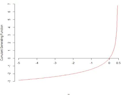
Figure (2.1) plots KS(u) versus u for the noncentral chi-square distribution with noncentrality

parameterαequal to unity. The values of the graph range from −∞asu↓ −∞to∞asu↑ 1 2, and

the functionKS(u) is always a strictly convex function when evaluated over (−∞,1/2) soK

00

S(u)>0

and the square root is well-defined.

2.6. NONCENTRAL CHI-SQUARE DISTRIBUTION 27

Figure 2.1: The cumulant generating functionKS(u) for noncentral Chi-square distribution versusu.

KS(u) is given by K0_S(u) = (1−2u)α+ 2αu (1−2u)2 + 2 (1−2u) = α−2αu+ 2αu+ 2(1−2u) (1−2u)2 = α+ 2−4u (1−2u)2 . (2.34)

Solve K0_S(u(s)) =s for u(s) in terms of s we get,

K0_S(u(s))−s = 0 α+ 2−4u(s) (1−2u(s))2 −s = 0 α+ 2−4u(s)−s(1−2u(s))2 (1−2u(s))2 = 0 α+ 2−4u(s)−s+ 4su(s)−4s u(s)2 = 0 4s u(s)2 + 4u(s)−4su(s)−2 +s−α = 0 4s u(s)2 + 4s1−s s u(s) + (−2 +s−α) = 0 u(s)2 +1−s s u(s) +−2 +s−α 4s = 0. (2.35)

The equation (2.35) is a quadratic and we may use the completing the square technique to solve it. Move the constant to the other side, add the square of half the coefficient of u(s) to both sides, factor the trinomial square and finally take the square root of both sides we get,

ˆ u(s) = −1−s 2s ± p (4 + 4sα) 4s . (2.36) Hence ˆ u(s) = −2 + 2s+ p (4 + 4sα) 4s or uˆ(s) = −2 + 2s−p(4 + 4sα) 4s . (2.37)

The positive root in (2.37) is not feasible since ˆu(s) would take values greater than 1/2 as s > 0. The cumulant generating functionKS(u) is only defined foru <1/2 and hence the saddlepoint ˆu(s)

is the negative root of the quadratic equation (2.35), ˆ

u(s) = ˆu(s, α) =− 1 4s

n

2−2s+p(4 + 4sα)o, s >0 and α_>0. (2.38) The plot of the saddlepoint ˆu(s) versussis shown in Figure (2.2) where the noncentrality parameter

α is equal to 1.

Figure 2.2: Saddlepoint function ˆu(s) versuss

2.6. NONCENTRAL CHI-SQUARE DISTRIBUTION 29 ˆ u(s) are given by KS(ˆu(s)) = αuˆ(s) 1−2ˆu(s) −log(1−2ˆu(s)) = −α 4s 2−2s+p(4 + 4sα) 1 + 1 2s 2−2s+p(4 + 4sα) −log n 1 + 1 2s 2−2s+p(4 + 4sα) o , (2.39) and K00_S(ˆu(s)) = −4(1−2ˆu(s)) 2_{+ 4(α+ 2−4ˆu(s))(1−2ˆu(s))} (1−2ˆu(s)4 = −4(1−2ˆu(s)) + 4(α+ 2−4ˆu(s)) (1−2ˆu(s))3 = −4 + 8ˆt(s) + 4α+ 8−16ˆt(s) (1−2ˆu(s))3 = 4α+ 4−8ˆu(s) (1−2ˆu(s))3 = 4α+ 4−8ˆu(s) n 1 + ₂1_s2−2s+p(4 + 4sα)o 3. (2.40)

The unnormalized first-order saddlepoint density approximation to f(s) is given by ˆ f1(s) = 1 q 2πK00_S(ˆu) expKS(ˆu)−usˆ . (2.41)

Figure (2.3), for instance, shows comparative plots of the true density f(s) (solid line) with the unnormalized first-order saddlepoint density approximation ˆf1(s) (dashed line) with various values

of the noncentrality parameter. Note that when increasing the values of the noncentrality parameter the relative error of each approximation stays bounded under suitable asymptotic regimes.

Note that when α = 0, the distribution reduces to the centrality case and the exact proba-bility density function for the noncentral distribution reduces to an exponential density with rate parameter 1₂, f(s) = 1 2exp −1 2s , s >0. (2.42)

For the saddlepoint approximation, we find ˆ u(s) = ˆu(s, α) =− 1 4s(4−2s) = − 1 2s(2−s) = − 1 2sη, s >0, (2.43)

whereη= 2−s. The cumulant generating functionKS(t) and the second derivative ofKS(t) about

the saddlepoint ˆu(s) are given by

KS(ˆu(s)) =−log(1−2ˆu(s)) =−log 1 + 1 sη , (2.44)

Figure 2.3: Exactf(s) (solid curve) and first-order saddlepoint density approximation ˆf1(s) (dashed line) versuss

2.6. NONCENTRAL CHI-SQUARE DISTRIBUTION 31 and K00_S(ˆt(s)) = 4−8ˆu(s) 1−2ˆu(s)3 = 4 1−2ˆu(s) 2, (2.45)

so that fors >0 and α= 0, the unnormalized first order saddlepoint density approximation tof(s) is given by ˆ f1(s) = 1−2ˆu(s)2 8π 1/2 expn−ln(1−2ˆu(s))−uˆ(s)so = 1 2 1−2ˆu(s) 1 2π 1/2 exp{−ln(1−2ˆu(s))}exp{−uˆ(s)s} = 1 2 1−2ˆu(s) 1 2π 1/2 1 1−2ˆu(s)exp{−uˆ(s)s} = 1 2π 1/21 2exp − − 1 2s(2−s) s = 1 2π 1/21 2exp{ 1 2(2−s) } = √ Γ(1) 2π11−12e−1 1 2exp n −1 2s o . (2.46)

The shape of ˆf1(s) in (2.46) is the same as that of f(s) in (2.42) but differs from f(s) in the

normalization constant. Using Stirling’s approximation for Γ(β), ˆ

Γ(β) =√2πββ−12e−β, (2.47)

and puting β = 1, we find ˆ

f1(s) =

Γ(1) ˆ

Γ(1)f(s) = 0.92214f(s). (2.48) This first order saddlepoint approximation to the noncentral chi-square density is also accurate for large α. Assume, for example, two large values for the noncentrality parameter, α = 10 and

α = 14 and use the R integrate function (see Crawley [11], p. 275 and Rizzo [85], p. 330) in the

stats package, the numerical integration for ˆf1(s) after converting it to a one-dimensional function

by fixing ˆu(s), KS(ˆu(s)) and K

00

S(ˆu(s)), yields a numerical value for the normalization constant c

given by1.035951underα= 10 with absolute error less than4.7e-06and 1.018552underα = 14 with absolute error less than 3.6e-07. Figure (2.4) shows a comparative plot of the true density