PRELIMINARY DRAFT COMMENTS WELCOME DO NOT CITE WITHOUT PERMISSION
Optimal Contract Length for Voluntary Land Conservation Programs
Xiaoxuan Chen* and Amy Whritenour Ando*
*Dept. of Agricultural and Consumer Economics, U. of Illinois at Urbana-Champaign, U.S.A.
Selected Paper prepared for presentation at the American Agricultural Economics Association Annual Meeting, Long Beach, California, July 23-26, 2006
Abstract: In many parts of the world, deteriorating environmental conditions have led policy makers to develop policies and programs aimed at promoting conservation practices on lands devoted to agriculture. Such programs have been studied by environmental economists, but little research has been done on the usefulness of strategically varying the conservation contract’s length. This paper uses theory and simulation to investigate the optimal contract length of land conservation programs when a policy maker tries to maximize the present discounted value of the stream of environmental benefits from the program. We find that contract length should vary with characteristics of the ecological processes that yield benefits from land retirement. Optimal contracts are longer when the environmental benefits in question – things like woodland
biodiversity – take time to develop. However, it is not typically optimal to have the indefinitely-lived contracts favored by some conservation groups, or even to offer contracts as long as the maturation period for the environmental services in question. In general, the optimal contract length depends on the trade off between an ecological effect (increasing the environmental benefits from one farmer) and an enrollment effect (increasing the number of farmers enrolled). Our findings also suggest that non-ecological regional characteristics (such as turnover rate and average farm income) could play an important role in the design of conservation programs.
1. Introduction
Over the last several decades, population and economic growth in many countries, including the United States, have resulted in the conversion of a significant amount of environmentally sensitive land to agricultural or urban uses. In many parts of the world (including the U.S., the European Union, China), deteriorating environmental conditions have created such concern that policy makers have developed policies and programs aimed at promoting conservation practices on lands devoted to agriculture. Given the large expenditures governments devote to such programs – $1.8 billion in the U.S., $6.8 billion in the EU, and $2 billion in China (Congressional Research Service, 2005) – there is value to exploring all dimensions along which the programs’ designs might be improved.
At the federal level of the U.S., the USDA Farm Service Agency’s (FSA) Conservation Reserve Program (CRP) has been the country's largest private-lands environmental improvement program. Its stated goal is to help agricultural producers preserve environmentally sensitive land, and thereby decrease erosion, restore wildlife habitat, and safeguard ground and surface water (USDA, 2004). At the state level, programs like state Conservation Reserve Enhancement Programs (CREPs) allow farmers to receive additional incentive payments for installing specific conservation practices. Through a CREP, farmers can receive annual rental payments and cost-share assistance to establish long-term, resource conserving covers on eligible land. There are also programs like the Wildlife Habitat Incentive Programs (WHIP) and Wetland Reserve Programs (WRP), which targets some specific characteristics of farmland.
Ever since the authorization of these land conservation programs, participation in voluntary conservation programs has attracted substantial research. Many papers have studied the minimum payment necessary to induce CRP enrollment (Tegene et. al., 1999), and some
have analyzed the optimal payment for a cost-effective CRP program (Parks and Schorr, 1997), but little research has been done on the potential impact of a varying CRP contract length and the relationship between the optimal CRP payment and the optimal CRP contract length. The few papers trying to fill this gap (Gulati and Vercammen 2005), unfortunately, oversimplifies the problem by assuming that land always returns to pre-contact use after a one-shot contract expires, and maximization of total environmental benefits can be achieved by getting the most
environmental benefits from a typical land owner. These assumptions are institutionally different from what is happening in the real world, where land owners often choose to extend the contract when the initial contract expires; and policy makers, aiming at total environmental benefits and faced with stringent budget constraint, may have to consider not only the benefits derived from one land owner but also the total number of enrollments.
An analysis of optimal contract length is valuable because it may provide policy makers with guidance regarding how to maximize environmental benefits in a cost-effective manner through adjustments in contract length as well as incentive payments. This paper provides that analysis, using theory and simulation to investigate the optimal contract length of land
conservation programs when a policy maker tries to maximize the present discounted value of the stream of environmental benefits from the program. Section 2 provides background on voluntary land conservation programs. Section 3 reviews the relevant literatures on
environmental benefits and conservation program design. Section 4 models the solution to a game between the government and farmers by finding a sub-game perfect equilibrium via backwards induction. The policy maker chooses a contract length and the associated payment. Given this contact length and payment, each farmer decides if she or he wants to enter into the contract. The farmer is allowed to re-contract and thus remain in the program after the initial
contract expires, but the policy makers’ spending must be kept within the limit of a pre-set budget constraint. The Bellman’s principle of optimality from dynamic programming is used to solve for the number of farmers that will enroll given a particular contract length and payment; this function informs the government’s contract design decision. Section 5 parameterizes the model and simulates the problem and its solution for several types of environmental benefits. Section 6 gives concluding comments and describes directions for further research.
2. Background on U.S. Voluntary Conservation Programs
As the country’s largest land conservation program, the CRP was established by the Food Security Act of 1985. From the beginning, the CRP has been tailored to the preservation of environmentally sensitive land and the reduction of erosion. Enrollment in CRP is voluntary. To be eligible, cropland must meet several standards in order to be considered as
environmentally sensitive. In exchange for enrollment, farmers receive a package of benefits including rental payments and cost-share assistance. FSA bases rental rates on the relative productivity of the soils within each county and the average dry land cash rent or cash-rent equivalent. In addition, FSA provides cost-share assistance to participants up to 50 percent of the participants’ costs in establishing approved land covers.
Enrollment in CRP increased rapidly once the program got underway. By the year 2003, nearly 34 million acres were enrolled at an annual rental cost of $1.8 billion. In exchange for retiring eligible land for 10-15 years, participants received an annual rental payment that averaged roughly $50/acre, and were reimbursed for half of the cost of establishing permanent cover (usually grasses or trees). The potential benefits of CRP to society as a whole, as well as to farmland owners, have made the program a recurring focus of farm program legislation.
The Conservation Reserve Enhancement Program (CREP) is an offshoot of the CRP. By combining CRP resources with state and private programs, CREP provides farmers with a financial package for conserving and enhancing the natural resources of farms. Enrollment in a state is limited to specific geographic areas and practices. CREPs differ across states, but many require a 10- to 15-year commitment to keep lands out of agricultural production. CREP
provides payments to participants who offer eligible land. A federal annual rental rate, including an FSA state committee-determined maintenance incentive payment, is offered, plus cost-share of up to 50 percent of the eligible costs to install the practice. Further, the programs generally offer a sign-up incentive for participants to install specific practices.
FSA uses CRP funding to pay a percentage of the program's cost, while state
governments provide the rest of the funds. States and private groups involved in the effort may also provide technical support and other in-kind services. To be eligible, land must be owned or leased for at least one year prior to enrollment, and must be crop land. Land must also meet cropping history and other eligibility requirements. Unlike CRP, CREP enrollment can be on a continuous basis, permitting farmers to join the program at any time rather than waiting for specific sign-up periods.
Among programs that target specific characteristics of farmland, the Wildlife Habitat Incentive Program (WHIP) and Wetland Reserve Program (WRP) have enjoyed great popularity. WHIP is a voluntary state-level program that encourages creation of high quality wildlife
habitats. Since WHIP began in 1998, nearly 14,700 participants have enrolled more than 2.3 million acres into the program. NRCS provides cost-share payments to landowners under these agreements that are usually 5 to 10 years in duration, depending upon the practices to be installed. They may also provide greater cost-share assistance to landowners who enter into agreements of
15 years or more for practices on essential plant and animal habitat. Priority is usually given to habitat areas for wildlife species experiencing declining or significantly reduced populations and practices beneficial to fish and wildlife that may not otherwise be funded.
WRP aims mainly at wetland conservation. The program provides an opportunity for landowners to receive financial incentives to restore, protect, and enhance wetlands by retiring marginal land from agriculture. The program offers three enrollment options. The first option is a conservation easement in perpetuity. Easement payments for this option are usually the
agricultural value of the land plus 100 percent of the costs of restoring the wetland. The second option is a 30-year contract where easement payments are 75 percent of what would be paid for a permanent easement plus 75 percent of restoration costs. The last option pays up to 75 percent of the cost of the restoration activity on contract of 10 years.
These programs yield a wide range of ecological benefits: erosion control, improved wildlife populations in grasslands and forests, and wetland services such as flood control and nutrient filtration that reduces excess nutrient levels in surface water. For at least some of these ecological services, the annual flow of benefits may increase as a function of time in a manner dictated by ecological processes. Variation in the nature of those functions might dictate that efficient conservation programs should offer contracts of varied lengths that depend on the nature of the service to be generated.
3. Literature Review
We base our work upon findings from literatures in two disciplines. In order to develop a reasonable specification for the environmental benefits function, we draw upon work in ecology
and plant and animal biology. In contrast, our model of the behavior of landowners and the policy maker is informed by the economics literature.
3.1 Environmental benefit functions: Hobbs and Harris (2001) shows the relative
abundance of species at five different stages of abandonment in old fields in Southern Illinois. Their results suggest that some species may need more than 25 to 40 years to be fully restored at one geographical location. This implies that the environmental benefits of land (of which
biodiversity is an important part) to a large extent depend on the time that the land is retired; for some benefits, it might be ecologically ineffective for a parcel of land to be retired for only a short period of time. This is true of benefits that hinge on the stature of vegetation.
The increase in vegetation stature has considerable ecological impact. MacArthur and MacArthur (1961) conduct a census of bird species in four U.S states differing in plant species composition, foliage height profiles and latitude to determine the potential influence of these factors on bird diversity. Results suggest that increasing vegetation stature is a primary driving force in the establishment of bird species.
Besides biodiversity, vegetation stature also plays an important role in the modification of the hydrological cycle and the establishment of soil horizons. Bosch and Hewlett (1982) study the impacts of afforestation on the water yields from small experimental catchments and show that the increased water use by forest cover compared to other smaller stature vegetation reduces water yields. In other words, trees dry out the soil, and bind it with their roots to a much greater extent than grass species. Results suggest that most forms of soil erosion can be reduced to a more significant extent if land is forested with trees than with smaller stature vegetation.
Vegetation stature, according to Forman and Godron (1986), increases in a sigmoid (a special case of the logistic function) or S-shaped fashion over time. The reason for this, as suggested by ecologists (Horn, 1971), is plants’ competition for light, which causes a general increase in the height of vegetation. Being taller gives a plant an obvious advantage in the competition for light. But that advantage comes at a cost. Very tall plants need to be strong enough to withstand tremendous forces like winds, snow and ice, forces from which shorter plants are protected. Thus, competition for light would lead plants to grow until the cost of further height offsets the advantage. Like the logistic function, height of vegetation rises up to and eventually levels off at a constant horizontal limit.
Given that many environmental benefits, such as biodiversity and reduction of soil erosion, are to a large extent determined by vegetation stature, and that the increase in vegetation stature follows a logistic function, it might be reasonable to assume that environmental benefits from land retirement also increase in a logistic fashion. However, the exact shape of a particular logistic function will depend on the identity of the ecosystem (e.g. vegetation matures more rapidly in some places) and the precise nature of the benefit (e.g. erosion control can be better provided for by low-stature grasses than can some kinds of wildlife populations.)
3.2 Economic studies of conservation programs: There have already been many studies
on land conservation programs. One set of papers focuses on the participation behavior of land owners and tries to identify the factors that might influence enrollment in such programs. For example, empirical work by Force and Bill (1989) relates adoption of CRP to a range of socioeconomic and attitudinal factors. Konyar and Osborn (1990) model the probability of farmer participation in the CRP as discrete choice problem; under their framework, a farmer participates if the expected utility of participation is greater than the expected utility of not
participating. They estimate the model using region-level data for the entire U.S., and find (among other things) that land value and expected net returns with and without participation influence the probability of CRP participation. Mclean-Meyinsse et al. (1994) explore the relative lack of participation in the CRP by small farmers who have highly erodible cropland. They find that complaints about low program payments tend to occur most frequently among farmers with larger farms and higher average land returns. Parks and Schorr (1997) present a conceptual model of a Northeastern farmer’s decision to participate in a program such as the CRP. The owner’s problem is modeled to be a choice of optimum amounts if any of land to enroll in the CRP program and to sell, respectively, in such a way as to maximize discounted profits including land sales. The model then supports an econometric study of participation in the CRP by Northeastern landowners, which finds that the CRP is relatively unimportant to agricultural land owners in metropolitan counties where land values outstrip program payments.
Since land conservation easements can be non-permanent, landowners are theoretically free to choose whatever practice to perform on their land once the contract expires. For this reason, post-contract land-use decisions of land owners have also become a focus of many research papers. For example, Kalaitzandonakes and Monson (1994) investigate the influence of economic, personal, and attitudinal factors on the intended conservation effort of a sample of 126 CRP contract holders after their contracts have expired. Economic factors were found to
dominate the decision about future conservation effort. Skaggs et al. (1994) use a multinomial logit model to identify characteristics influencing New Mexico CRP participants’ post-CRP land use plans. Of the 811 participants surveyed, 21% have expressed intention of going back to farming, 40% plan to re-enroll and the rest of them are undecided. Results indicate post-CRP land use intentions will vary with attributes reflecting characteristics of the land enrolled,
socioeconomic variables, and participant attitudes (concern for erosion and interest in permanent land retirement). Johnson and Segarra (1995) evaluate four policy alternatives for CRP lands, upon expiration of the current contracts, in Hale County, Texas. Results suggest that if CRP contracts are extended at the current average rental rate, 40 percent of the current enrollment would be expected to return to crop production, while 66 percent would return to crop production if the program is eliminated. Cooper and Osborn (1998) estimate the CRP re-enrollment
decisions by farmers. They apply econometric and simulation methods to a survey of over 8,000 CRP contract holders, and find that up to 50% of current CRP acreage can be renewed at less than the current average CRP cost of $50 per acre (though achieving near 100% contract renewal would be expensive.)
Are these programs worth the money we spend on them? There has been some research done on the environmental effects of land conservation programs. Goodwin and Smith (2003) estimate a model of cross-sectional, county-level data encompassing agricultural production and soil erosion both before and after the introduction of the CRP and the rapid expansion of crop insurance programs. The study confirms the CRP significantly reduced erosion in areas where farmers have participated. Unfortunately, Wu’s (2000) estimate of the slippage effects of CRP shows that for each one hundred acres of cropland retired under the CRP in the central United States, twenty acres of non-cropland were converted to cropland, offsetting 9% and 14% of CRP water and wind erosion reduction benefits, respectively.
Studies of the design of a cost-effective CRP program have also considered the role of option values in determining appropriate rental payment, and have considered how to exploit targeting strategies to improve cost-effectiveness. Tegene et al. (1999) model a landowner’s decision to convert farmland to urban use as an irreversible investment under uncertainty, and
use that model to identify the appropriate level of conservation compensation By employing the real option framework, this research modifies earlier work on easement valuation by accounting for the role of land owner uncertainty in predicting future returns from development. They find that conservation easements are under priced and the payments offered in conservation programs might not be large enough to attract land threatened by development. Schatzki (2003)’s empirical tests of conversion from agriculture to forest confirm his theoretical hypothesis that landowners consider the option values when making decisions to convert agricultural land to conservation status. His work provides guidance to those designing CRP payments, since he finds higher uncertainty in returns to all potential uses and lower correlation between shocks to agricultural and forest returns decreases the likelihood of conversion to forest through CRP. Wu, Zilberman, and Babcock (2001) compared the economic, environmental, and distributional impacts of four targeting strategies (targeting of resources for benefit-cost ratios, benefits alone, benefit per resource unit, and low costs) and identify circumstances under which different strategies are most useful.
Amongst all this work, there has been little discussion about the role that contract length might be able to play in the design of a cost-effective land conservation program. In the
literature on carbon sequestration, however, some researchers have begun to explore the determinants of optimal length for carbon offset contracts. Gulati and Vercammen (2005a) propose a one-shot decision model of carbon contract length. In the model, the authors assume that land always return to pre-contact use once the contract expires. Furthermore, there is only a single representative farmer, so that total environmental benefits are positively related to the chosen contract length. The authors conduct simulation analysis; their results suggest that a higher carbon price or a higher discount rate could lead to a longer optimal contract and that the
greater the similarity between the technologies used in and out of the contract, the longer the optimal contract.
This model of the optimal contract length of carbon sequestration, although insightful, has two key features that limit its usefulness for modeling conservation contracts. First, since it models only a single round of contracting, it is unable to explore the impact of expected
enrollment turnover at the re-contracting time on the optimal contract length. Second, the policy maker cares about total environmental benefits rather than the benefit from a single (even though typical) farmer. As we will see in the next section, total benefits from a group of heterogeneous farmers are not necessarily increasing in contract length. Enrollment considerations play an important factor in determining the optimal contract design.
4. Model
We construct a theoretical model to determine the optimal design of land-conservation contracts – both contract length and payment – when the policy maker maximizes environmental benefits subject to a budget constraint, and farmer participation is voluntary. We use backwards induction to solve the policy maker’s problem given farmers’ behavior
4.1 Landowners’ enrollment decisions: The payoff to a farmer from not entering the
conservation program in question is one period of farming income plus the present discounted value of the maximized stream of payments derivable from the land. Similarly, the payoff from entering the program would be the present value of the program’s payment plus the maximized stream of payment discounted back from the end of the contract. Here the “maximized stream of payments” is defined as the payoff to the farmer from doing whatever is optimal on his or her
land, which could include (but is not limited to) farming income, conservation program rental payment, or revenue from commercial development.
Given contract length L and rental payment P, a land owner chooses whether to enter into the land conservation program or not. We denote the farmer’s individual benefit from farming as Bf which is assumed to follow a Brownian motion process (without drift) over time,
dZ t dBf( )=σt where dZ =dt 2 ) ( (1) That is, an individual farmer’s income from farming will undergo chance fluctuation over time. Let V denote the discounted value of payoffs to the farmer from making his or her choice optimal between (a) entering conservation programs and (b) staying out. If choosing (b) is optimal, then V r B V = f + + 1 1 (2) since choosing (b) will yield a payoff of Bf in this period and will in expectation lead to exactly
the same choice between (a) and (b) in the next period. Therefore we have that
f B r V ⎟ ⎠ ⎞ ⎜ ⎝ ⎛ + = 1 1 (3)
If choosing (a) is optimal, then
V r P V L ⎟ ⎠ ⎞ ⎜ ⎝ ⎛ + + = 1 1 (4)
since choosing (a) will yield a fixed rental payment P during the contract period and will in expectation lead to exactly the same choice between (a) and (b) once the contract expires (at the end of contract length L). Therefore we have that
(
)
(
r)
P r V L L ⎥ ⎦ ⎤ ⎢ ⎣ ⎡ − + + = 1 1 1 (5)We may set
(
)
(
r)
P r B r L L f ⎥ ⎦ ⎤ ⎢ ⎣ ⎡ − + + = ⎟ ⎠ ⎞ ⎜ ⎝ ⎛ + 1 1 1 11 and solve for the relationship between contract
length L and payment P that will make a farmer indifferent between farming and entering land conservation programs, 1 ) 1 ln( ) ln( ln + ⎥ ⎦ ⎤ ⎢ ⎣ ⎡ + − + − = r rP rB B B L f f f . (6) Alternatively, the relationship can be written as
(
)
L f f f f(
)
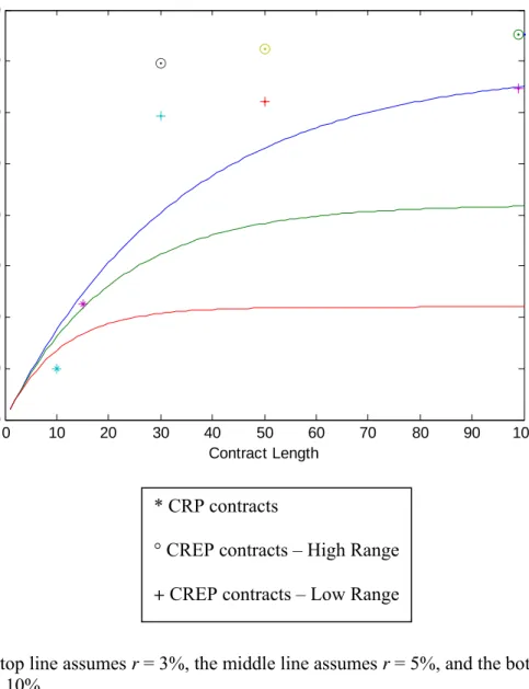
L L r r B r B B B r r r P − ⎥ = + − + − ⎦ ⎤ ⎢ ⎣ ⎡ + − + = 1 1 1 1 1 ) 1 ( (7)To explore the relationship between program payment and contract length, we show in Figure 1 a plot of the combinations of lump-sum1 program payments and associated contract lengths that will make a farmer indifferent between farming and entering a conservation agreement. The contour lines represent indifference curves for different discount rates. On the same graph, we show the combinations of payment and contract length that have actually been offered under CRP and the Illinois CREP. One might expect that these combinations would roughly lie along an indifference curve, but in fact they do not. This represents a small empirical mystery. It could be that policy makers fail to understand the necessary tradeoffs between
payments and contract lengths, and inadvertently offer excessively high (in the case of CREP) or low (in the case of CRP) payments for the shorter contracts. Alternatively, these distortions may reflect the presence of a more complex mechanism-design strategy; we explore this possibility in another paper.
The fraction of farmers that enter the program is determined by the number of farmers for whom the payoff to (a) exceeds the payoff to (b):
(
)
(
)
L f L B r P r r ⎟ ⎠ ⎞ ⎜ ⎝ ⎛ + > ⎥ ⎦ ⎤ ⎢ ⎣ ⎡ − + + 1 1 1 1 1 or(
)
(
1)
1 1 1 0 1 > ⎟ ⎠ ⎞ ⎜ ⎝ ⎛ + − ⎥ ⎦ ⎤ ⎢ ⎣ ⎡ − + + f L L B r P r r (8)We assume that the net incomes from farming are normally distributed across farmers according to ~ Ν
(
µ,σ2)
f B . Then we have(
)
(
)
L f L B r P r r ⎟ ⎠ ⎞ ⎜ ⎝ ⎛ + − ⎥ ⎦ ⎤ ⎢ ⎣ ⎡ − + + 1 1 1 1 1 ~(
)
⎪⎭⎪⎬ ⎫ ⎪⎩ ⎪ ⎨ ⎧ ⎟ ⎠ ⎞ ⎜ ⎝ ⎛ + ⎟ ⎠ ⎞ ⎜ ⎝ ⎛ + − ⎥ ⎦ ⎤ ⎢ ⎣ ⎡ − + + Ν 2 2 1 1 , 1 1 1 1 ) 1 ( µ σ r r P r r L L (9)And the fraction of farmers for which equation (8) holds is given by
(
)
) , ( 1 1 1 1 1 1 1 1 P L r r P r L =Φ ⎪ ⎪ ⎭ ⎪ ⎪ ⎬ ⎫ ⎪ ⎪ ⎩ ⎪ ⎪ ⎨ ⎧ ⎟ ⎠ ⎞ ⎜ ⎝ ⎛ + ⎟ ⎠ ⎞ ⎜ ⎝ ⎛ + − ⎥ ⎦ ⎤ ⎢ ⎣ ⎡ + − + Φ σ µ (10)As can be seen from Equation 10, the fraction of farmers that will enter CRP or CREP depends on the payment P, contact length L, mean of net income from farming µ, variance of farming income σ2 and the discount rate r. Holding other variables constant, a higher payment will lead to more enrollments. Similarly, for a given payment, a longer contract length will result in fewer enrollments; for any given payment and contract length, a higher average farming income raises the opportunity cost of enrollment and therefore results in fewer enrollments; a larger variance means that net income from farming (and therefore the opportunity cost of enrollment) is quite different across farmers, thus limiting the possibility of attracting a large number of farmers by offering a universal payment and contract length. The influence of the discount rate is unclear from the above formulation.
4.2 Policy maker’s contract design problem: We assume that the government seeks to
maximize the total present discounted value of environmental benefits from all enrolled land. The program is infinitely lived, with contracting opportunities every L years. The government may only choose a single contract to offer all farmers, and the total cost of the program is subject to a budget constraint. As long as a given parcel is enrolled in the conservation program, benefits from that parcel continue to evolve according to the environmental benefits function B(t). Once the parcel drops out of enrollment (i.e. a re-contracting opportunity is not accepted), the flow of benefits from the parcels falls to zero; if the parcel is later re-enrolled, benefits again begin to flow with the time counter re-set to zero.
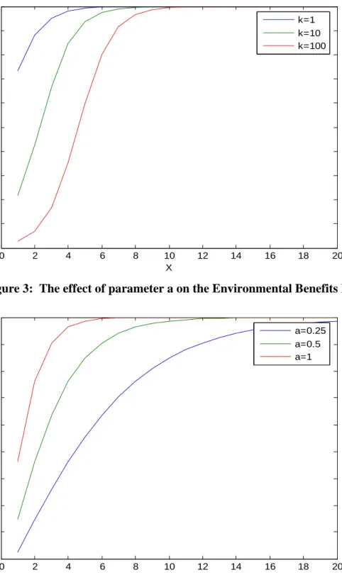
We specify the environmental benefits function to be given by al ke l B − + = 1 1 ) ( . As shown
in Figures 2 and 3, the shape of the environmental benefits function depends on the parameters a and k. A typical logistic function rises up to and eventually levels off at a constant horizontal limit. The function first increases at an increasing rate, and then increases at a decreasing rate. That is, the curve changes from being convex to concave. The rate at which a logistic function rises to its limiting value is completely determined by the exponential function in the
denominator, in particular, by the parameters a and k. Specifically, the parameter k affects the location where the change from being convex to concave occurs. The Y intercept gets lower as k increases, which suggests that the starting value of environmental benefits is smaller for a higher k. On the other hand, the parameter a affects the curvature of the logistic curve. The logistic function becomes more concave as a increases, which means that the environmental benefits would increase more abruptly for a higher value of a. By varying these two parameters, our model can simulate conditions in a wide variety of ecological situations.
Equation 10 gives the fraction Ф(L,P) of all farmers that will accept a contract offering of a given P and L. We assume there are n farmers in total, and denote N = n Ф(L,P) as the number of farmers that enroll for a given contract. Since ecological heterogeneity and targeting is not a primary focus of this paper, we assume that all farmers in the region have the same
environmental benefits function so that these functions can be aggregated across farmers. Because individual farmers’ values of Bf evolve randomly with Brownian motion, the identity of
the farmers that enroll in each contracting period will not be the same (though as long as the Brownian process does not have drift, the number of enrollments will not change.) The parameter α gives the percentage of enrollments that are new at each contracting period – something we refer to as the “churning factor.”2
With this notation in place, we are able to write the government’s objective function. It seeks to maximize the present discounted value of environmental benefits from all enrolled parcels given infinite rounds of contracting:
∑
= ⎟ ⎠ ⎞ ⎜ ⎝ ⎛ + L l l l B r N 0 ) ( 1 1 ) ( 1 1 ) 1 ( ) ( 1 1 1 1 2 0 l B r N l B r r N l L L l l L l L∑
∑
= = ⎟ ⎠ ⎞ ⎜ ⎝ ⎛ + − + ⎟ ⎠ ⎞ ⎜ ⎝ ⎛ + ⎟ ⎠ ⎞ ⎜ ⎝ ⎛ + +α α∑
∑
∑
= = = ⎟ ⎠ ⎞ ⎜ ⎝ ⎛ + − + ⎟ ⎠ ⎞ ⎜ ⎝ ⎛ + ⎟ ⎠ ⎞ ⎜ ⎝ ⎛ + − + ⎟ ⎠ ⎞ ⎜ ⎝ ⎛ + ⎟ ⎠ ⎞ ⎜ ⎝ ⎛ + + L L l l L L l l L L l l L l B r N l B r r N l B r r N 3 2 2 2 0 2 ) ( 1 1 ) 1 ( ) ( 1 1 1 1 ) 1 ( ) ( 1 1 1 1 α α α α +...
(11)The first line of Equation 11 shows the environmental benefits derived from the first contracting period, the second line shows those from the second period, and so on. The
environmental benefits at each contracting period equal the benefits from all new enrollments plus those from all the lands that are already in the programs. The total environmental benefits are derived by adding up the discounted environmental benefits of each period. Using theorems of infinite geometric series, Equation 11 can be reduced to
(
)
∑
(
)
∑
∞ = + = ⎥ ⎥ ⎦ ⎤ ⎢ ⎢ ⎣ ⎡ ⎟ ⎠ ⎞ ⎜ ⎝ ⎛ + − ⎥ ⎦ ⎤ ⎢ ⎣ ⎡ − + + 0 ) 1 ( ) ( 1 1 1 1 1 1 i L i iL l l i L B l r r N α α (12)Therefore the government’s problem can be expressed as
(
)
∑
(
)
∑
∞ = + = ⎥ ⎥ ⎦ ⎤ ⎢ ⎢ ⎣ ⎡ ⎟ ⎠ ⎞ ⎜ ⎝ ⎛ + − ⎥ ⎦ ⎤ ⎢ ⎣ ⎡ − + + 0 ) 1 ( , 1 ( ) 1 1 1 1 1 i L i iL l l i L L P N r r B l Max α α (13) subject to(
)
(
)
(
r)
nP(
P L)
BC r L P P r n L L i iL ≤ Φ ⎥ ⎦ ⎤ ⎢ ⎣ ⎡ − + + = Φ ⎟ ⎠ ⎞ ⎜ ⎝ ⎛ +∑
∞ = , 1 1 1 , 1 1 0 (14)where BC is the budget constraint and Equation 14 suggests that the discounted accumulated spending on land conservation programs must be kept within a preset budget limit.
This problem is too complex to derive analytical results. Hence, we simulate optimal program design in several situations to gain insight into the optimal contract design problem.
5. Simulations and Results
We use parameter values as follows. The average net farm income per acre is just above $100 from the year 1997 to 2004 (USDA 2005), which we will use as our mean of net income from farming, µ. There are no reported figures on the variance of farming income, σ2, but since farming income can vary largely from year to year (USDA 2005), we will assume a reasonably large standard deviation of farming income, σ = $100. The discount rate is assumed to be 5%,
which is the most common rate that is available to agricultural financing (Federal Reserve Board 2005).
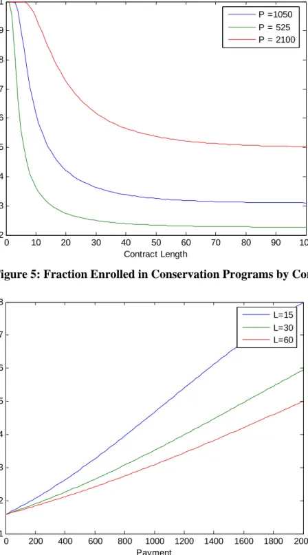
Under these baseline assumptions, a simulation was carried out to characterize the relationship among conservation program participation, environmental benefits from a single landowner, total benefits of a region, contact length and rental payment. In our model, the fraction of farmers that is going to enter land conservation programs depends on rental payment as well as contract length. As shown in Figure 4, if we hold the rental payment constant, enrollment will decrease as contract length increases. The reason is that a long-term contract locks the farmer into a fixed agreement. Hence there are more years of foregone opportunities, and this increased opportunity cost has to be compensated by higher payment. As Figure 5 illustrates, the lump-sum rental payment necessary to induce enrollment increases as a decreasing rate as the contract length goes up; this is because discounting lowers the present value of the opportunity cost of a foregone year of income as the year moves further into the future.
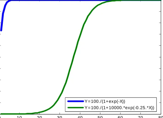
Total environmental benefits from the program depend on the shape of the environmental benefits function. Figure 4 shows the shape of the function two different types of ecological processes. The blue line represents the case where environmental benefits start out high and level off after very short periods of time (e.g., erosion control benefits from perennial grass) while the green line reveals the process where it takes much longer for the benefits to reach maximum (e.g., wildlife populations dependent upon mature trees). Hence, the optimal contract length might not always be the same for different functional forms of the environmental benefits, and in order to maximize social welfare, the policy maker would need to take into account the differences in the ecological processes that underlie conservation programs.
The government’s problem is to maximize the environmental benefits from land at a given region. On the one hand, the policy maker would prefer to keep a single parcel in conservation status for a sizable number of years in order to fully reap the benefits from land retirement; on the other hand, a longer contract length may lead to fewer enrollments, which may adversely affect the total environmental benefits that can be derived from the region. Similarly, the policy maker has an incentive to raise the rental payment given that its objective is to maximize environment benefits through land retirement, but the budget constraints will limit its ability to increase the payment. The tradeoffs between contract length and rental payment would make the policy maker’s task more complicated than if only rental payment is considered.
The policy implications of introducing contract length into the government’s decision making process can be illustrated using Figure 5, where a given level of total environmental benefits can be achieved by numerous combinations of payments and contract lengths. Under the traditional framework that considers only variation in payment, the only way to increase total environmental benefits is to increase rental payment. In contrast, when contract length can vary, we show that total environmental benefits can be increased through either a reduction or an increase in total rental payment. For example, a longer contract will lead to more payment for each farmer but few enrollments, so the total payments might not be necessarily higher, but the total environmental benefits can be higher if the accumulation effect of environmental benefits from each farmer dominates the enrollment effect. Therefore under our framework, it is quite possible for the regulators to achieve a given (or even higher) total environmental benefits for less money. It all depends on the trade off between the ecological effect (environmental benefits from one farmer) and the enrollment effect (the number of farmers enrolled).
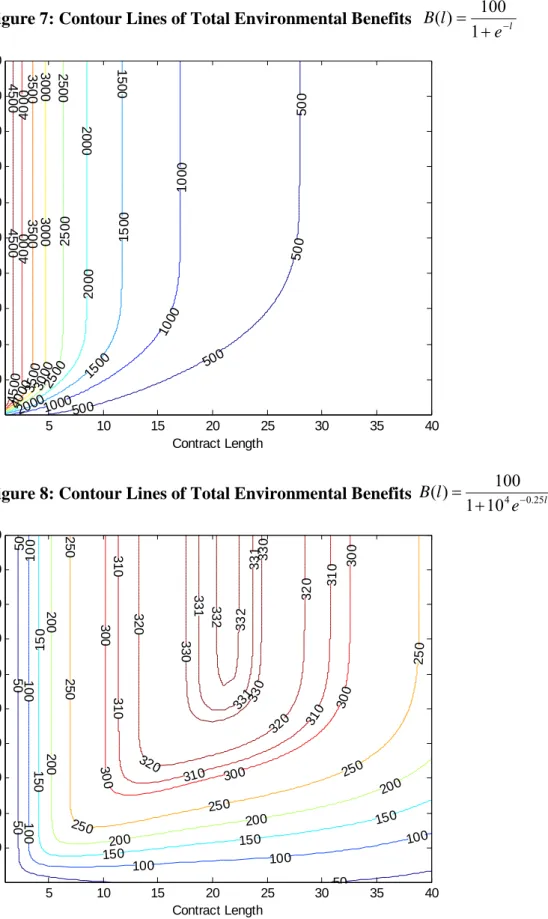
Figure 6 also shows how the optimal contract length can differ for different
environmental benefit functions. Figure 7 corresponds to the ecological process represented by the blue line (grasslands) and Figure 8 corresponds to that represented by the green line
(forest) of Figure 4. Once we add in the budget constraint illustrated in Figure 9, we can solve for the combinations of contract length and payment that would maximize the total environmental benefits given that budget constraint. For example, suppose we have a budget constraint equal to $10,000. In the case of the grassland benefits (shown in Figure 7), the optimal contract length would be one year. Essentially, the contract length should be as short as possible, since we do not allow for a zero or negative contract length. In contrast, in the case of woodland benefits (shown in Figure 8) the optimal contract length is 21 years. Clearly, the optimal contract length can vary widely with the underlying ecological process. However, the best contract length is not a
function simply of any particular feature of the environmental benefits function. For example, in both of our scenarios, the optimal contract length was shorter than the time needed for the flow of benefits to level off at its maximum.
To explore the determinants of optimal contract length in greater detail, we simulate the impact on optimal contract design of non-ecological regional characteristics and the nature of the environmental benefit function. Specifically, we show how L* varies with the rate of turnover in the identity of parcels that enroll in sequential enrollment periods, the mean value of the net income from farming, and the starting value of the environmental benefits.
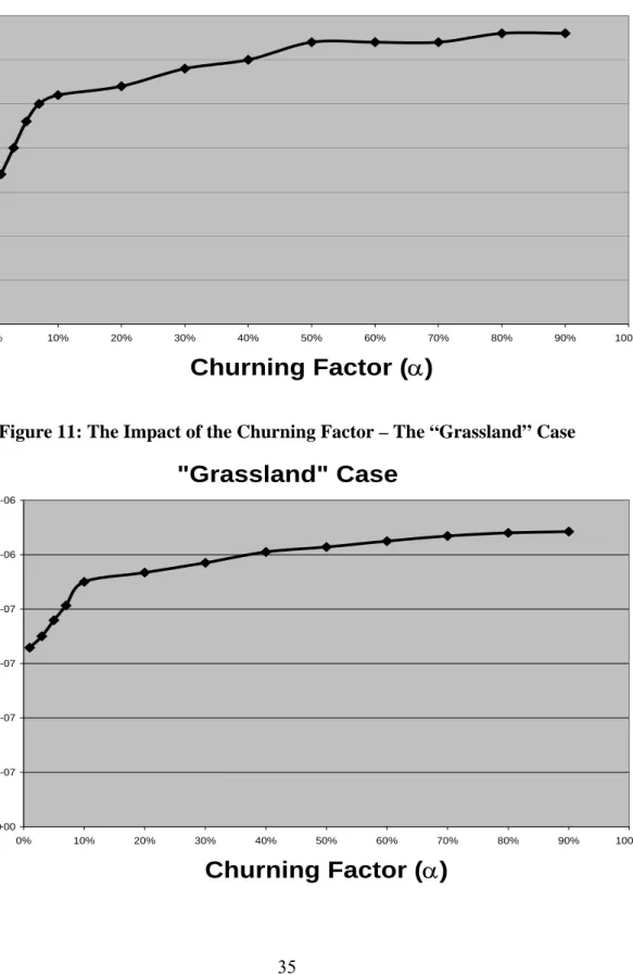
Figure 10 shows graphs of the impact of the churning factor (α) on optimal contract length (L*) for two different types of ecological settings. As can be seen from these graphs, for both ecological processes, the churning factor is positively related to the optimal contract length. Policy makers should consider offering longer contracts while designing these programs if there
is evidence suggesting that the turnover rate on such programs is high. Another interesting thing to note is that the optimal contract length is increasing at a much faster rate when the churning factor is below 10% than when it goes beyond 10%. For example, in the “forest” case, the
optimal contract length increases by 9 years (from 17 years to 26 years) when the churning factor increases from 1% to 10%, while a change in the churning factor all the way from 10% to 90% only lengthens the optimal contract by another 7 years (from 26 years to 33 years). The same is true for the “grassland” case, but in this setting the optimal contract length is close to zero for all values of α. This finding suggests that the effect of churning on the optimal contract length is small for ecological services that mature quickly.
Figure 11 shows the impact of mean farm income (µ) on optimal contract length (L*) for the same two types of ecosystems. We observe a negative relationship between mean farm income and the optimal contract length. This suggests that policy makers should consider offering shorter contracts in areas where the average farmer makes more money from farming. Under our framework, a farmer determines whether to enroll into conservation programs based on his or her comparison between the payoffs from farming and the payoffs from enrollment. In regions where agricultural productivity is higher, it is more difficult for policy makers to
convince farmers to give up farming. As a result, more “sweeteners” (in the form of either a higher payment or a shorter contract) need to be offered to these farmers in order to get them interested in these conservation programs. In the “forest” setting, optimal contract length does not fall very much over low levels of income, but between $600 and $1000/acre the optimal contract length falls by about 50% (from 25 years to just more than 12), after which point L* becomes robust again to changes in income. In the “grassland” case, the optimal contract length is always extremely low; any changes in L* with respect to mean farm income occur between
very low and medium levels of income. Our results suggest that while average farm income is generally inversely related to optimal contract length, the scale and pattern of that impact depends on the underlying ecological process.
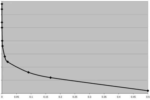
Finally, we investigate how optimal contract length varies with characteristics of the environmental benefit function. One important feature of that function is its Y-intercept, which indicates the level of annual benefits at the beginning of the restoration process as a fraction of the maximum benefits that will accrue each year once the benefit matures. Essentially, this is the starting value of the environmental benefits. The higher the starting value, the less time it takes for the ecological process to mature. Figure 12 suggests that shorter contracts should be offered when conservation aims to provide environmental benefits that mature quickly. In particular, our findings suggest that a change in the fraction of maximum annual benefits at T=0 has a big influence on the optimal contract length, which falls very rapidly as initial benefits increase from nothing to as low 10% of matured annual benefits.
6. Conclusions
We find that the optimal contract length depends on the trade off between an ecological effect (environmental benefits from one farmer) and an enrollment effect (the number of farmers enrolled). On the one hand, the policy maker would prefer to keep a single parcel in
conservation status for a sizable number of years in order to fully reap the benefits from land retirement; on the other hand, a longer contract length may lead to fewer enrollments, which reduces total environmental benefits from the region.
This study provides guidance for the manner in which contract length should be varied with characteristics of the ecological processes that yield benefits from land retirement. Optimal
contracts are longer when the environmental benefits in question – things like wetland services or woodland biodiversity – take time to develop. However, it is not typically optimal to have the indefinitely-lived contracts favored by some conservation groups, or even to offer contracts as long as the maturation period for the environmental services in question; high payments must be offered to induce farmers to accept such contracts, which would severely limit the number of acres enrolled.
Our findings also suggest that non-ecological regional characteristics could play an important role in the design of conservation programs. Specifically, optimal contracts are longer in regions where the turnover rate on conservation programs is high, although the effect of churning on the optimal contract length is small for ecological services that mature quickly. Moreover, we find that average farm income is inversely related to optimal contract length, due to the fact that more incentives are needed to attract higher-productivity farmers into
conservation programs. Finally, these impacts on optimal contract length are different across different ranges of regional characteristics. Thus, to increase the benefits society reaps from the money spent on conservation programs, policy makers should take into account the direction of influence by these ecological and non-ecological characteristics, and work to determine the actual levels of these characteristics.
References
Bosch, J. M. and Hewlett, J. D. 1982. “A Review of Catchment Experiments to Determine the Effect of Vegetation Changes on Water Yield and Evapotranspiration.” Journal of Hydrology 55: 3-23.
Capozza, D. and Li, Y. 1994. “The Intensity and Timing of Investment: The Case of Land.” American Economic Review 84: 889-904.
Cooper, J. C. and Osborn, Y. C. 1998. “The Effect of Rental Rates on the Extension of
Conservation Reserve Program Contracts.” American Journal of Agricultural Economics, 80(1): 184-194.
Force, D., and Neison B. 1989. “Participation in the CRP: Implications of the New York experience.” Journal of Soil and Water Conservation 44: 512-516.
Forman, R. T., and M. Godron. 1986. Landscape Ecology. New York: John Wiley & Sons, Inc. Goodwin, B. K. and Smith, V. H. 2003. “An Ex Post Evaluation of the Conservation Reserve,
Federal Crop Insurance, and Other Government Programs: Program Participation and Soil Erosion.” Journal of Agricultural and Resource Economics, 28(2): 201-216.
Gulati, S. and Vercammen, J. 2005a. “The Optimal Length of an Agricultural Carbon Contract.” University of British Columbia Working Papers.
Gulati, S. and Vercammen, J. 2005b. “The Economic Value of Flexible-length and Interim Measurement Soil Carbon Contracts.” University of British Columbia Working Papers. Hobbs, R. J. and Harris, J. A. (2001) “Restoration Ecology: Repairing the Earth’s Damaged
Ecosystems in the New Millennium.” Restoration Ecology 9: 239 - 246.
Johnson, P. N. and Segarra, E. 1995. “An Evaluation of Post Conservation Reserve Program Alternatives in the Texas High Plains.” Journal of Agricultural and Applied Economics, 27(2): 556-64.
Kalaitzandonakes, N. G. and Monson, M. 1994. “An Analysis of Potential Conservation Effort of CRP Participants in the State of Missouri: A Latent Variable Approach.” Journal of Agricultural and Applied Economics, 26(1): 200-208.
Konyar, K., and Osborn, C. T. 1990. “A National-Level Economic Analysis of Conservation Reserve Program Participation: A Discrete Choice Approach.” Journal of Agricultural Economics Research 42: 5-12.
MacArthur, R. H., and J. W. MacArthur. 1961. “On Bird Species Diversity.” Ecology 42:594-598.
Mclean-Meyinsse, P. E., Hui, J., and Joseph, R. Jr. 1994. “An Empirical Analysis of Louisiana Small Farmers’ Involvement in the CRP.” Journal of Agricultural and Applied
Economics 26: 379-385.
Parks, P. and Schorr, J. 1997. “Sustaining Open Space Benefits in the Northeast: An Evaluation of the Conservation Reserve Program.” Journal of Environmental Economics and Management, 32:85-94.
Schatzki, T. 2003. “Options, Uncertainty and Sunk Costs: An Empirical Analysis of Land Use Change.” Journal of Environmental Economics and Management 46: 86-105.
Skaggs, R. K., Kirksey, R. E. and Harper, W. M. 1994. “Determinants and Implications of Post-CRP Land Use Decisions.” Journal of Agricultural and Resource Economics, 19(2): 299-312.
Tegene, A., Wiebe, K. and Kuhn, B. 1999. “Irreversible Investment under Uncertainty: Conservation Easements and the Option to Develop Agricultural Land.” Journal of Agricultural Economics, 50(2): 203-219.
Wu, J.. 2000. “Slippage Effects of the Conservation Reserve Program.” American Journal of Agricultural Economics, 82(4): 979-992.
Wu, J., Zilberman, D. and Babcock, B. 2001. “Environmental and Distributional Impacts of Conservation Targeting Strategies.” Journal of Environmental Economics and Management 41: 333-350.
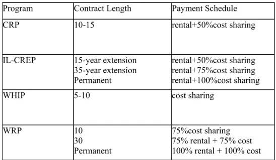
Table 1: Contract Options in Land Conservation Programs
Program Contract Length Payment Schedule
CRP 10-15 rental+50%cost sharing
IL-CREP 15-year extension
35-year extension Permanent
rental+50%cost sharing rental+75%cost sharing rental+100%cost sharing
WHIP 5-10 cost sharing
WRP 10 30 Permanent 75%cost sharing 75% rental + 75% cost 100% rental + 100% cost
Figure 1: Indifference Curves over Lump-Sum Program Payment and Contract Length 0 10 20 30 40 50 60 70 80 90 100 0 500 1000 1500 2000 2500 3000 3500 4000 Contract Length P a y m ent
Note: The top line assumes r = 3%, the middle line assumes r = 5%, and the bottom line assumes r = 10%.
* CRP contracts
° CREP contracts – High Range + CREP contracts – Low Range
Figure 2: The effect of parameter k on the Environmental Benefits Function 0 2 4 6 8 10 12 14 16 18 20 0 0.1 0.2 0.3 0.4 0.5 0.6 0.7 0.8 0.9 1 X Y k=1 k=10 k=100
Figure 3: The effect of parameter a on the Environmental Benefits Function
0 2 4 6 8 10 12 14 16 18 20 0.55 0.6 0.65 0.7 0.75 0.8 0.85 0.9 0.95 1 X Y a=0.25 a=0.5 a=1
Figure 4: Fraction Enrolled in Conservation Programs by Contract Length
Figure 5: Fraction Enrolled in Conservation Programs by Contract Payment
0 200 400 600 800 1000 1200 1400 1600 1800 2000 0.1 0.2 0.3 0.4 0.5 0.6 0.7 0.8 Payment F ra c ti on E n ro ll ed L=15 L=30 L=60 0 10 20 30 40 50 60 70 80 90 100 0.2 0.3 0.4 0.5 0.6 0.7 0.8 0.9 1 Contract Length F rac ti on E n ro ll ed P =1050 P = 525 P = 2100
Figure 6: Environmental Benefits Function for Two Different Processes 0 10 20 30 40 50 60 70 80 0 10 20 30 40 50 60 70 80 90 100 x f( x ) Y = 100./(1+ ex p(-X)) Y = 100./(1+ 10000.*ex p(-0.25.*X))
Figure 7: Contour Lines of Total Environmental Benefits
Figure 8: Contour Lines of Total Environmental Benefits
50 50 50 50 1 00 100 100 100 100 100 1 5 0 150 150 150 150 200 200 200 200 200 250 250 250 250 250 25 0 300 3 0 0 300 30 0 3 0 0 310 310 310 31 0 3 1 0 320 320 320 3 2 0 330 33 0 3 3 0 331 331 3 3 1 332 3 3 2 Contract Length P a y m ent 5 10 15 20 25 30 35 40 1000 2000 3000 4000 5000 6000 7000 8000 9000 10000 500 500 50 0 5 00 1000 10 00 1 0 00 15 00 1 5 0 0 1500 20 00 2 0 0 0 2000 25 00 2 5 0 0 25 00 30 00 30 00 30 00 35 00 35 00 35 00 4 0 0 0 4 0 0 0 40 00 4 500 4 500 45 00 Contract Length Pa y m e n t 5 10 15 20 25 30 35 40 1000 2000 3000 4000 5000 6000 7000 8000 9000 10000 l e l B − + = 1 100 ) ( l e l B 4 0.25 10 1 100 ) ( − + =
Figure 9: Contour Lines of Budget Constraints 5000 5000 5000 5000 1000 0 1000 0 1000 0 10000 20 00 0 20 00 0 20 000 40 00 0 40 00 0 60 00 0 60 00 0 80 00 0 8 00 00 1 00 00 0 Contract Length P a y m ent 5 10 15 20 25 30 35 40 1000 2000 3000 4000 5000 6000 7000 8000 9000 10000
Figure 10: The Impact of the Churning Factor – The “Forest” Case
"Forest" Case
0 5 10 15 20 25 30 35 0% 10% 20% 30% 40% 50% 60% 70% 80% 90% 100%Churning Factor (
α
)
O
p
ti
m
a
l C
o
nt
ra
c
t Lengt
h
Figure 11: The Impact of the Churning Factor – The “Grassland” Case
"Grassland" Case
0.0E+00 2.0E-07 4.0E-07 6.0E-07 8.0E-07 1.0E-06 1.2E-06 0% 10% 20% 30% 40% 50% 60% 70% 80% 90% 100%Churning Factor (
α
)
O
p
ti
m
a
l C
o
nt
ra
c
t Le
ngt
h
Figure 12: The Impact of the Mean Farm Income – The “Forest” Case
"Forest" Case
0 5 10 15 20 25 30 0 100 200 300 400 500 600 700 800 900 1000Mean Farm Income (
µ
)
O
p
ti
m
a
l C
ont
ra
ct
Lengt
h
Figure 13: The Impact of the Mean Farm Income – The “Grassland” Case
"Grassland" Case
7.8E-07 8.0E-07 8.2E-07 8.4E-07 8.6E-07 8.8E-07 9.0E-07 9.2E-07 9.4E-07 9.6E-07 0 100 200 300 400 500 600 700 800 900 1000Mean Farm Income (
µ
)
O
p
ti
m
a
l C
o
nt
ract
Lengt
h
Figure 14: The Impact of the Fraction of Maximum Annual Benefits at T=0 0 5 10 15 20 25 30 35 0 0.05 0.1 0.15 0.2 0.25 0.3 0.35 0.4 0.45 0.5