Why do Worker-Firm Matches Dissolve?

No. 2006–57

WHY DO WORKER-FIRM MATCHES DISSOLVE?

By Anne C. Gielen, Jan. C. van Ours

June 2006

Why do worker-firm matches dissolve?

Anne C. Gielen

Jan C. van Ours

June 9, 2006

Abstract

In a dynamic labor market worker-firm matches dissolve frequently causing workers to separate and firms to look for replacements. A separation may be initiated by the worker (a quit) or the firm (a layoff), or may result from a joint decision. A dissolution of a worker-firm match may be inefficient if it can be prevented by wage renegotiation. In this paper we study worker separations in the Dutch labor market. From an analysis of matched worker-firm data we conclude that both quits and layoffs are less likely to occur in high quality matches. We also find that workers with a high propensity to quit are offered higher wages to prevent them to quit. Similarly, workers with a high layoff probability give up some of their wage to prevent them from being laid-off. Despite these wage renegotiations some inefficiency in separations remains. However, there is a clear difference between quits and layoffs. Whereas inefficient quits are rare inefficient layoffs occur frequently. These phenomena may be related to downward wage rigidity. While it is easy to renegotiate higher wages to prevent quits it is much more difficult to renegotiate lower wages to prevent layoffs even if that would overall be beneficial to the workers involved.

JEL codes: J31, J63, M51.

Keywords: Separations, Quits, Layoffs, Matched worker-firm dataset.

∗_{Department of Economics, Tilburg University, CentER, Institute for Labor Studies (OSA); email:}

[email protected]. Corresponding author, address: Department of Economics, Tilburg University, P.O. Box 90153, NL–5000 LE Tilburg, The Netherlands. Phone: +31 13 466 3216. Fax: +31 13 466 3042.

†_{Department of Economics, Tilburg University, CentER, IZA and CEPR; email: [email protected].}

The authors would like to thank the Ministry of Social Affairs and Employment for the use of the AVO dataset, and Frederic Vermeulen, Marcel Kerkhofs, Norma Coe and Marco Francesconi for their helpful suggestions. Anne Gielen gratefully acknowledges financial support from the Institute for Labor Studies (OSA).

1

Introduction

In a dynamic labor market workers change their labor market position frequently. When a worker enters a job the wage is negotiated on the basis of the expected quality of the match between worker and firm. Both parties take advantage of the match and split-up the match-specific surplus through wage negotiations. The match-match-specific surplus may be affected by shocks and change over time. Therefore, the employment relationship is continuously reevalu-ated. A relationship may be terminated if the value of the match for either one or both parties falls below the value of an outside option. As a result, a separation may be initiated by a worker or a firm, or result from a joint decision. The larger the value of the match-specific surplus, the lower the probability that a separation occurs. A separation initiated by the worker is denoted a quit, a firm-initiated separation is denoted a layoff.

A separation is inefficient if it could have been prevented through wage renegotiation. If a worker leaves a firm because of a higher outside wage the firm might have prevented this by offering a higher wage too. That would have reduced the firm’s part of the match surplus but could still have been profitable if the match surplus of a newly hired worker is even lower. Similarly, the firing of a worker is inefficient if a wage reduction would have prevented the dismissal and the worker would be better off when the outside wage is lower than the reduced wage. A separation is efficient if the match surplus became negative or if it is too small for compensation, i.e. insufficient to compensate the worker who wants to leave or the firm that wants to fire a worker. So, whether a separation is efficient or not depends on the size of the match surplus, the size of the shocks and the possibility to renegotiate the wage. If wages cannot be renegotiated some separations may be inefficient while others are efficient. The distinction between quits and layoffs is related to wage rigidity, i.e. either the worker or the firm is not willing or able to renegotiate the sharing rule governing the costs and returns to firm-specific human capital (Becker (1962) and Parsons (1972)). If wages are fully flexible a separation is always efficient and the distinction between quits and layoffs is irrelevant (Burdett (1978), Jovanovic (1979), Mortensen (1988)).1 _{Nevertheless, in this case the separation is most}

1_{However, McLaughlin (1991) has shown that even in the case of efficient separations, there can be a} meaningful distinction between quits and layoffs, which is based on who initiates the separation by demanding

likely classified as a quit because a layoff would require a formal action by the employer and is often a costly event due to employment protection legislation.

In this paper we investigate why worker-firm matches dissolve. From a simple theoretical model we derive three predictions. First, separations are less likely to occur if the joint match specific surplus is high. Second, some separations may be inefficient because they occur when there is still a positive match-specific surplus. Third, inefficient separations may be avoided through renegotiations. In our analysis based on Dutch matched worker-firm data we investigate to what extent we can find empirical evidence for these theoretical findings.

In the empirical part of the paper we define a proxy for the match surplus to investigate whether indeed matches are less likely to dissolve when the match surplus is high. We use the match surplus as explanatory variables in separation estimates. Indeed we find that both quits and layoffs are less likely to occur when the match surplus is high. Then, we investigate whether indeed wages are renegotiated. Here we use the expected probability to quit or being laid-off as an explanatory variable in wage growth estimates finding that a high quit probability has a positive effect on wage growth while a high layoff probability has a negative effect. From this we derive that indeed some wage renegotiation occurs. Finally, we use the results of the empirical analysis to find an indication of the extent to which quits and layoffs that occurred where efficient or inefficient.

The set-up of this paper is as follows. In section 2 we present a theoretical model about efficient and inefficient separations and give a brief review of previous literature. Section 3 describes the dataset we use and presents some stylized facts. In section 4 the results of our empirical analysis are presented. Finally, section 5 concludes.

2

Theory and previous research

2.1

Theoretical model

Our theoretical model is based on Farber (1999). We assume that the employment relationship between the workeriand the firmj at time t generates a match-specific revenue. The value of

a wage revision. Then, quits are worker-initiated separations that result from censored wage increases, while layoffs are firm-initiated separations that result from censored wage cuts.

the production generated by the worker equalsVijtand the wage of the worker equalsWijt. For the firm the match generates a surplus which is equal to the difference between the production value and the wage of the worker:

S_ijtF =Vijt−Wijt (1)

For the worker the match generates a surplus which is equal to the difference between the wage and the alternative incomeAt which the worker could earn outside firm j:

SW

ijt=Wijt−At (2)

The alternative incomeAtis the market wage for given worker characteristics, such as education level. The total match-specific surplus is equal to the sum of the workers’ surplus and the firm surplus:

Sijt=SijtF +SijtW =Vijt−At (3) Or, in other words, total match-specific surplus is equal to the value of the production minus the alternative earnings of the worker.2 _{The surplus is divided between worker and firm through}

wage negotiations that generate a sharing rule such that firms receive a shareβijt and workers receive a share (1−βijt), with 0 ≤ β ≤ 1. The wage is equal to the alternative earnings plus the share of the match-specific surplus:

Wijt=At+ (1−βijt)Sijt (4)

Now consider what happens if we introduce labor market dynamics by allowing for the occur-rence of two types of shocks to the surplus, shocks to the alternative earnings and shocks to the match-specific productivity. First we consider a shock to the alternative earnings which may lead to a quit:

At+1 =At+θt+1 (5)

where θ can be considered as an external shock, which is a random variable with mean zero drawn from the distribution functiong(θ). If no wage renegotiations are possible and changing

2_{Note that in this simple set-up the firm could hire a new worker at wage A}

tand produce Vjt=At so there

is no match surplus. Hiring and firing costs for the firm and separation costs for the worker are assumed to be zero for computational simplicity. However, introducing positive hiring and firing costs and separation costs does not change the predictions of the model.

labor market position is costless, a worker quits if the alternative income exceeds the wage he receives in the firm:

At+1 > Wijt

θt+1 >(1−βijt)Sijt (6)

Equation (6) shows that the worker is less likely to quit when the value of the workers’ surplus is larger.

Similarly, some match-specific shock may occur which gives rise to a layoff. This match-specific shockφ is a random variable with mean zero drawn from the distribution function f(φ). The shock affects the value of production of the worker in the firm:

Vij,t+1 =Vijt+φt+1 (7)

The firm will layoff the worker if the firm’ surplus falls below zero:

Vij,t+1 < Wijt

φt+1 <−βijtSijt (8)

Equation (8) indicates that the worker is laid off if the negative shock is sufficiently large to outweigh the firm’s share of the surplus.

In this model we can identify both efficient and inefficient separations. An efficient separa-tion (ES) occurs if the joint surplus of the match falls below zero after the shocks have occurred. The efficient separation condition can be defined as follows:

Sij,t+1 <0

Sijt< θt+1−φt+1 (9)

A separation is efficient if the positive shock to the alternative wage and the negative match-specific shock are sufficiently large to offset the value of surplus. Note that efficient separations are independent of the firm’s share of the joint match surplus. Efficient separations can be subdivided in efficient quits and efficient layoffs. An efficient quit (EQ) occurs if the external

shockθ exceeds the value of the worker surplus and if the sum of both shocks exceeds the joint match surplus, i.e.,

Sijt< θt+1−φt+1 and θt+1 >(1−βijt)Sijt (10) Since the sum of both the external and the match-specific shock is larger than the initial match surplus, the joint match surplus in the next period falls below zero. Hence, there is no renegotiation possible such that the worker can be compensated for the external shock to alternative earnings. Similarly, an efficient layoff (EL) occurs if the value of the match-specific shock exceeds the firm surplus and if the sum of both shocks exceeds the joint match surplus, i.e.,

Sijt< θt+1−φt+1 and φt+1 <−βijtSijt (11) Such a layoff is efficient since the sum of both shocks is too large, such that there is no renego-tiation possible such that the firm can be compensated for the match-specific shock.

A separation is inefficient if total match surplus is positive. If the shock to the alternative earnings is sufficiently large it will be profitable for the worker to quit, but this also destroys the positive firm surplus. Similarly, if the match-specific shock is sufficiently negative if will be profitable for the employer to fire the worker, but this also destroys the positive worker surplus. Hence, the inefficient quit (IQ) condition can be defined as follows:

(1−βijt)Sijt< θt+1 < Sijt+φt+1 (12)

Similarly, the inefficient layoffs (IL) can be defined as:

θt+1−Sijt< φt+1 <−βijtSijt (13) Renegotiation of the wage may prevent inefficient quits and layoffs. As soon as the sum of both shocks is smaller than the joint match surplus, βijt can be renegotiated (βij,t+1) in order

to redistribute the joint surplus. Then, the number of quits and layoffs will be reduced.3

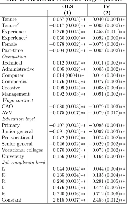
A graphical illustration of efficient and inefficient separations is given in Figure 1.4 _Here,X

denotes the original match, before some shock has occurred. On the axes, the match-specific (φ)

3_{Indeed, Hall and Lazear (1984) show that an ex ante fixed surplus sharing rule will lead to excess separations.} 4_{’ST’ represents a stay, ’EQ’ and ’IQ’ an efficient and inefficient quit, ’EL’ and ’IL’ an efficient and inefficient} layoff, and ’ES’ indicates an efficient separation.

and external (θ) shock are presented. If the shocks are smaller than the current match surplus for each party (βijtSijt for the firm and (1−βijt)Sijt for the worker), the match is maintained. If at least one of the shocks is larger, renegotiation of the surplus division is necessary to avoid a match dissolution. The diagonal line between−SijtandSijtindicates a set of combinations of

SW

ijt and SijtF that can be reached when the division of the total match surplus is renegotiated, i.e. changing βijt. To the north-west of this diagonal we observe efficient separations, since there is no successful renegotiation possible that can compensate the shocks and thereby can prevent a worker-firm match to split up. Note that a positive match-specific shock does not lead to wage renegotiations, since it does not lead to a negative surplus for either party, therefore neither party has an incentive to initiate a separation. A similar argument goes for a negative alternative earnings shock.

Overall, the main message of the theoretical model is threefold. First, separations are less likely to occur if the joint surplus is high. Second, some separations may be inefficient because they occur when there is still a positive match-specific surplus. Third, inefficient separations may be avoided through renegotiations. In the analysis below we will investigate to what extent we can find empirical evidence for these theoretical findings. Before presenting the results from our empirical analysis we first give a brief review of previous literature.

2.2

Previous literature

In the theoretical model a separation is less likely to occur if the match-specific surplus is large. Quits are less likely to occur if the worker surplus is large, layoffs are less likely if the firm surplus is large. Residuals from wage regressions can be used as proxies for the worker surplus. A wage residual measures the difference between the current wage and the wage that could be obtained in a similar job given the worker and firm characteristics. Obtaining an approximation of the firm surplus is a more difficult task, because information about individual worker productivity is absent in a lot of datasets. However, if total match surplus is shared between the worker and the firm, a larger worker surplus also implies a larger firm surplus.5

5_{Note that if a positive wage residual indicates that a worker is overpaid compared to his peers the layoff} probability increases with the wage residual.

In this paper, we use the wage residual as a proxy for match quality. Three theoretical approaches explain why the residual of a wage regression is a good indicator of the quality of the match. The first explanation is from the human capital theory (Becker (1964)), since there may be individual-specific differences in the amounts of specific training, which may affect earnings. The human capital theory predicts that wage residuals are negative for job market entrants and positive for high-tenure workers. That is, young workers pay for investments in specific training by receiving lower wages initially, but higher wage growth later in the career. The second explanation for match quality being reflected in the residual is from the job matching theory (Jovanovic (1979)). Worker-firm match quality is assumed to be unknown ex ante. This theory predicts an increase in the value of the match component as workers acquire tenure on the job, since the value of the match is revealed over time and only good matches are maintained. According to both theories, tenure can be used as a predictor of firm-specific skills (Mincer (1974)). Parent (2002) provides evidence for the importance of firm-specific human capital, but finds little support for the job matching theory. Yamaguchi (2003) however does find significant matching effects. Finally, differences in wage residuals can be explained by the job search theory (Burdett (1978)). This theory states that employed workers continue searching for jobs in which they are offered a higher wage. The importance of job search for match quality is empirically confirmed by Yamaguchi (2003) who finds that most of match quality growth is due to job search.

Both the job matching theory, as well as the human capital theory and the job search theory, predict that matches with high wage residuals are less likely to be dissolved. This prediction is empirically confirmed by Altonji and Shakotko (1987), Borland and Lye (1996), Barth and Dale-Olsen (1999) and Yamaguchi (2003). Not only individual worker effects, but also firm effects that can make up part of the wage residual appear to affect worker separations. In general, high-wage firms seem to have lower worker turnover than low-wage firms (Powell et al. (1994), Galizzi and Lang (1998), Haltiwanger and Vodopivec (2003) and Dale-Olsen (2006)). A natural experiment is done in Abowd and Finer (1997) where changing regulations impose that all workers that are going to be laid off should be notified in advance. Again it is found that workers in firms with high firm fixed effects stay longer with the firm, even after the layoff

notification, than workers in firms with low firm fixed effects. Though the matching model (Jovanovic (1979)) states that it is especially the bad matches with negative wage residuals that are dissolved, Lazear’s raiding model (Lazear (1986)) predicts the opposite. In this model rival firms will spot high productivity workers and ’raid’ them. Hence, it is especially good matches that dissolve, through quits. Support for this theory is found by Garen (1989).

While most studies focus on separations in general, some studies distinguish between quits and layoffs in order to examine the (different) effect of the wage residual on worker- and firm-initiated separations. The theoretical model in the previous section predicts that the wage residual affects both quits and layoffs in a similar way, because the match surplus is shared between the worker and the firm. This prediction is confirmed by Altonji and Shakotko (1987) who find that the wage residual has a negative effect on both quits and layoffs. Also, Pfann (2006) finds that workers with low wage residuals are more likely to be laid off. However, a more recent study by Perticara (2004) shows that workers with a strongly negative wage residual are more likely to quit, while a worker with a strongly positive wage residual is more likely to be laid off by the firm. This indicates that a high wage residual is not always an indicator of a large surplus but could also be an indicator of workers being overpaid.

The theoretical model in the previous section predicts that workers and firms may want to renegotiate the wage when a separation is imminent in order to avoid inefficient match dissolutions.6 _{As a result of this renegotiation, wages will change. Several studies have paid}

attention to wage dynamics that result from separations. In general, it is found that workers who quit experience wage gains (e.g. Perez and Rebollo (2005); Light (2005)) while dismissed workers experience wage losses (see Farber (1999) for an overview) compared to workers who remained with the firm. However, few studies have investigated how wages are affected by the ex-ante probability of separation. Workers may be willing to renegotiate their wage when they face the risk to loose their job. Few studies have paid attention to the relationship between wage changes and the risk of firm close down. In general, wage renegotiations can be positively and negatively related to the risk of firm closing. On the one hand, workers can agree with wage

6_{Malcomson (1999) provides an overview of types of contracts and renegotiation possibilities. The discussion} also includes an overview of the (adverse) effects renegotiation may have on individual worker decisions, such as investing in human capital.

concessions in order to avoid firm closing and displacement. On the other hand, in the face of firm closing workers can claim higher wages to compensate for the layoff risk. Hamermesh (1988, 1991) presents a model in which wage changes that are necessary to prevent plant closing are negotiated. He finds that a negative demand shock has to be met with a far below-average wage increase to avoid firm closing. Accepting only small wage cuts is unlikely to be successful in avoiding a shutdown. This might explain workers resistance to wage concessions, since they have to accept a substantial wage cut with certainty in return for only a small reduction in the firm closure probability. Nevertheless, Blanchflower (1991) does find that workers in unionized workplaces who expect to be made redundant earn 9% less than workers who do not face this risk. A more recent paper by Carneiro and Portugal (2006) estimates a simultaneous-equations model of firm closing and wages using Portuguese data to analyze how wages are adjusted to adverse economic shocks that increase the layoff probability. They also find that the fear of job loss generates wage concessions rather than claims for a higher wage. All in all, it seems that workers are willing to accept wage concessions in order to prevent job loss. Similarly, if a worker is offered attractive contracts by alternative employers, the current employer may be willing to pay the worker a higher wage in order to retain him. After making a decomposition of wage growth Yamaguchi (2005) finds that employers are indeed willing to renegotiate the workers’ wage: 20% of wage growth for young workers is due to an improved bargaining position of the worker. We are not aware of any other study investigating firms’ willingness to renegotiate the wage in order to prevent a worker from quitting. In our paper we investigate this issue in more detail, where we investigate the change in wages as a response to expected quit and layoff probabilities.

When firms are unable to renegotiate the wage, inefficient separations will occur (Hashimoto and Yu (1980) and Hall and Lazear (1984)). However, even with flexible wages, inefficiency in separations can remain (Ramey and Watson (1997)). Note that efficient separations only occur when the highest wage the firm is willing to pay is lower than the lowest wage the worker is willing to accept and hence are independent of the current wage. However, due to asymmetric information, the firm does not always know the outside option of the worker, and the worker does not always know at what wage the firm will decide to replace him. Hence, in the presence

of asymmetric information renegotiation can no longer guarantee that only efficient separations occur. Several studies have pointed out that in the presence of asymmetric information it is very difficult to design an incentive compatible contract that generates efficient layoffs and efficient quits (Hall and Lazear (1984); Haltiwanger (1984)). One paper that studies inefficiency in separations is a recent paper by Hall (2005) which states that the sticky-wage inefficient-separations model does not describe the modern U.S. labor market. He uses aggregated data to show that layoffs remained almost constant during different phases of the business cycle. Apparently, modern employment relationships are generally terminated in the joint interest of the worker and the firm and hence, inefficient separations are not an important phenomenon in the modern U.S. economy.7 _{We are not aware of any other study investigating the extent}

of inefficiency in separations. In this paper, we will add to this small literature by using wage growth information to determine which separation is efficient and which is inefficient.

3

Data and stylized facts

3.1

Data

We use administrative information of workers and firms in the Netherlands over the period 1993-2002.8 _{The dataset contains matched worker-firm information and has a repeated}

cross-section set-up where each cross-cross-section contains information at two points in time, one year apart. Every year about 1900 firms and 44,000 workers are sampled. The dataset does not contain financial information about the firms such as value added, output, profits, capital and investment.9

7_{However, Shimer (2005) discerns from this conclusion by stating that in the analysis no attention is paid to} separations which are privately inefficient.

8_{These are the AVO data; “AVO” is in Dutch: “Arbeidsvoorwaardenontwikkeling” (see Arbeidsinspectie} (2003). The data are from the Working Conditions Survey of the Dutch Ministry of Social Affairs and Em-ployment. Unless otherwise indicated the graphs and tables in this paper are based on the AVO data. In the analysis information from 1999 is not used since in this year no distinction is made between quits and layoffs.

9_{This is due to the fact that the data were designed to study changes in wages and therefore only information} from the wage administration of firms was obtained. See Gielen and van Ours (2005, 2006) for a Table with AVO means for several variables and Arbeidsinspectie (2003) for a detailed variable description and more information about the sample design. Since the 1993 sample contains no information on public sector workers, we excluded firms from this sector in other years as well. Firms from the service sector and semi-public sectors were included in all samples.

The data are obtained by means of a two stage sampling procedure. In the first stage, a sample of firms is drawn from the Department of Social Affairs internal firm register that is roughly similar to the firm register of the Dutch statistical office. The sample is drawn using a stratified design – by economic sector and firm size. In the second stage, a sample of workers within each firm is drawn. Information is collected from the wage administration of the firm for two distinct moments in time: October of the year of the survey (denoted byt) and October of the previous year (denoted byt-1). A distinction is made between workers working at the firm at both moments in time (‘stayers’), workers working at the firm only at time t (‘entrants’), and workers working at the firm only at time t-1 (‘leavers’).10 _{The share of sampled workers}

within a firm decreases with firm size and depends on several workers categories (covered by collective bargaining contract or not; stayer/leaver/entrant). The sample size was increased if certain conditions were not met.11 _{Because of this sampling design, some worker categories}

were underrepresented in the sample.

The reason for a separation is reported by the firm. A separation is denoted a quit if the worker has started a job in another firm, if he has become self-employed or if he has resigned himself. Similarly, a separation is denoted a layoff if the worker is dismissed or left the firm because of being disabled. We focus on prime-age workers, aged between 30 and 50, in order to abstain from other separations such as retirements or students leaving a holiday job.12

3.2

Stylized facts

Table 1 shows some stylized facts concerning the separate exit routes. For comparison, some stylized facts for stayers are presented in the first column. It appears that large part of the workforce concerns stable employment relationships. Separations are a decreasing function of

10_{Note that since workers are observed at two moments in time, we do not know the number nor the} char-acteristics of the workers who were hired after October of year t−1 and left the firm before October of year

t.

11_{At least 10 employees had to be covered by a collective bargaining agreement and 10 not; the minimal} number of stayers, entrants and leavers had to be at least 8. This sampling design results at the firm level in random samples from subgroups of workers discerned by working in the firm in October of year t or t-1, or both, and covered by collective bargaining (or not).

12_{For example, young workers may enter and leave the workforce randomly, because they work few hours} next to their educational obligations. Similarly, old workers may leave the workforce because of retirement or health considerations, which need not be influenced by financial reasons.

tenure. Quits occur more often among low experience workers in small firms. Layoffs are more prevalent among low educated workers in low complexity jobs. Finally, quits seem to behave procyclical, whereas layoffs do not show a clear cyclical pattern.

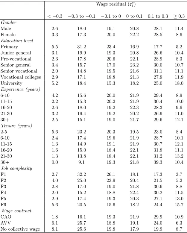
Figure 2 illustrates the average gross hourly wage for workers who stay with the firm and workers who leave. It appears that workers who quit earn relatively low hourly wages. This confirms the theoretical prediction that workers with low wage residuals are more likely to quit. However, there does not seem to be a difference in the average hourly wage earned by workers who stay with the firm compared to workers who are laid off.

4

Empirical analysis

In this section we investigate in more detail which worker-firm matches most likely dissolve. We distinguish between separations initiated by the worker and the firm. First, we estimate a wage-equation in order to obtain wage residuals that can be used as a proxy for match quality. Then, we include this measure in a separations equation in order to determine the effect of match quality on worker-firm separations. Finally, we investigate whether wages are renegotiated next period in order to prevent the dissolution of valuable worker-firm matches.

4.1

Wage estimation

We estimate a Mincerian wage equation for prime-age workers where the log of the gross hourly wage (wij) denoted in 1993 Dutch guilders is explained by worker, job and firm characteristics.13 Since the panel element of our dataset is limited, we cannot include individual fixed effects in the wage equation. Therefore, the wage residual includes both individual ability and match quality information.14

wij =Xijπ+νj+γτij +εij (14) where Xij is a vector of personal (i) and job characteristics (j), νj are firm fixed effects, τij represents job tenure andεij is an error term.

13_{The gross hourly wage is corrected for inflation. 1 guilder equals approximately 0.454 euro. Note that}

wij =ln(Wij), whereWij is the gross hourly wage.

14_{Actually, having ability and match quality in one measure is appropriate, since it avoids having zero match} quality for workers who never changed jobs.

The results of the wage estimation can be found in the first column of Table 2.15 _{We find that}

wages are lower for females, part-time workers and low educated workers. Moreover, it appears that tenure and potential experience have a positive but decreasing effect on wages. According to previous studies, general human capital accounts for a larger part of wage growth than specific human capital. In order to correct for potential endogeneity of tenure and experience we re-estimate the wage equation using an instrumental variables (IV) approach, where tenure and experience are instrumented by deviations of the means for the observations in a given occupation-job complexity level-education level combination.16 _{When looking at the estimates}

for tenure and experience from the IV-estimation, it appears that the OLS-estimates indeed suffer from an estimation bias. Hence, hereafter we will continue to use the IV-estimation results.17

The wage residual that is assumed to represent the workers’ surplus is obtained by comparing the current wage in the firm to the market wage obtained from the wage equation evaluated at zero tenure. This is done because tenure at the current firm is not rewarded by another firm when changing jobs. As a result, the residual consists out of an unobserved individual match effect (µij) – equal to the sum of the individual wage residual evaluated at current tenure and the firm fixed effect – and the tenure effect (γτij):

ε∗

ij =bνj +εbij+γτb ij =µbij +γτb ij (15)

Table 3 illustrates how the wage residual is spread over the different demographic groups by showing the percentage of the workforce that belongs to a certain residual interval. It appears

15_{We exclude cases with tenure and experience of one year or less in order to make sure the estimates are not} affected by temporary contracts. Sensitivity analysis show that the exclusion of these cases does not affect the results. Potential experience is computed as the worker’s age minus the years of schooling attended minus 6. Note: year dummies drop out because of the firm fixed effect.

16_{This approach is based on Altonji and Shakotko (1987), who provide a clear overview of the nature of} the bias. This method is also the preferred method of Dustmann and Pereira (2005) who compare several IV methods in order to avoid estimation biases in wage estimations. Since we do not have a panel dataset, we cannot take individual means of tenure and experience. Therefore, we construct a given job type, based on occupation, job complexity level and education, and compute average tenure and experience for this ”job”.

17_{We do not take into account potential endogeneity of the part-time work dummy variable. According to} traditional labor supply theory, part-time work is considered endogenous since the wage level determines the number of hours worked. However, in practice, the opposite may be more likely: people choose to work either part-time of fulltime and then investigate what wage is available for them. Therefore, we do not instrument the variable for part-time work.

that the wage residual is higher on average for high-experience and high-tenure workers in large firms. This is due to the firm fixed effect that is increasing with firm size and the tenure effect that is increasing with tenure. Moreover, high-residual workers seem to be more likely to stay with the firm, while low-residual workers are more likely to separate. This provides preliminary evidence in favor of the predictions from the theoretical model.

4.2

Worker separations

In this section we investigate which worker-firm matches are dissolved. In particular, we de-termine how separations are affected by the wage residual, which is used as a proxy for match surplus. Figure 3 shows how the match surplus, represented by the wage residual obtained in the previous section, affects worker-firm separations. In general, it appears that workers with low wage residuals are more likely to quit or to be laid off. For layoffs this is mainly due to the tenure effect. The effect of the unobserved individual match effect on quits is U-shaped: quits are more likely to occur for workers at both ends of the match effect distribution.

In order to investigate the effect of the residual on dissolving worker-firm matches we es-timate logit models for separations, quits and layoffs including the wage residual in the set of regressors. We compute robust standard errors, where we correct for correlation of the error terms within firms. Moreover, since we use a generated regressor, i.e. the wage residual, in the analysis, we adjust the asymptotic covariance matrix along the lines of Murphy and Topel (1985). The effect of the total wage residual (ε∗

ij) is presented in panel A of Table 4. Linear effects (panel A.1.) enter the model significantly only in the layoff equation. When asymmetry in the effects is allowed for (panel A.2.), we find that the effect of the residual on separations is U-shaped: workers at both ends of the wage residual distribution are most likely to quit. Lower end workers may be more likely to search for another job since they are underpaid. This underpayment may be due to a bad worker-firm match (Jovanovic (1979)). Also, the high quit propensity for low-residual workers may be due to a low firm fixed effect, which is an indicator for future wage growth (Galizzi and Lang (1998)). The effects for workers at the top end of the distribution provide evidence for the raiding model (Lazear (1986)): high residual workers are more likely to quit since firms will spot the high ability of these workers and raid them.

This U-pattern is not found for layoffs, that seem to occur mainly among workers with negative wage residuals. An LR-test indicates that introducing quadratic effects (panel A.3.) does not improve the model. In panel B of the Table, the individual effects of the separate residual ele-ments are investigated. Tenure effects appear to reduce all separations, as predicted by Parsons (1972), while larger match effects (µij) only reduce layoffs (panel B.1.). When asymmetry in the separate effects is allowed for (panel B.2.), we find that the U-shaped effect of the residual on quits and separations (from panel A.2.) is due to a U-shaped pattern in the match effect. However, the layoff probability is only affected by negative match values. This is in line with Bishop (1990), who finds that layoff rates are negatively related to match quality measures. Again, introducing quadratic effects (panel B.3.) does not improve the model.

The parameter estimates in Table 4 show that separations are not a linear function of the wage residual. In order to identify the separation pattern in more detail we use a flexible spline function. Then we estimate a logit model for quits and layoffs separately, where the quit or layoff decision is dependent among other things on the wage residual, conditional upon the residual interval it belongs to. The results are used to predict the quit and layoff probability. Figure 4 illustrates the relationship between the wage residual and quit and layoffs, respectively. Again we find the U-shaped pattern for quits. On the other hand, layoffs appear to be a random process, i.e. independent of the residual. Although we find some significant effects for the wage residual on layoffs, the overall layoff probability is very small: average predicted layoff probability is 1.19, while the average predicted quit probability is 6.18. Consequently, the effects of the wage residual on the layoff probability are even smaller. Moreover, there does not seem to be a relation between the quit probability and the layoff probability.

4.3

Wage renegotiations

The previous analysis has provided us with estimated quit and layoff probabilities. We are in-terested in whether firms and workers respond to these separation probabilities by renegotiating the match surplus. Our dataset contains two wage observations of workers that are present in the firm at both the first date (t) and the second date (t+ 1). Assuming that the wage at the

first date is determined by a match-specific component (αij)18, the wage at the second date is determined by this match-specific component, a general effect representing national shocks (ψ) and individual-specific expected probabilities to quit ( ˆPq) or to be laid-off ( ˆPl). So, wijt =αij and wij,t+1 =αij+ψ+δ1Pˆq,i+δ2Pˆl,i.19 Taking first differences we find

∆wijt =ψ+δ1Pˆq,i+δ2Pˆl,i

The expected probabilities ˆPq and ˆPl are an indication of the quality of the match in relation to external and match-specific shocks. If ˆPq is high the worker is underpaid and/or the shock to the outside option is large and the individual has a large incentive to quit. If ˆPl is high the worker may be overpaid or subject to a negative match-specific shock and has a high probability to be laid off. If wage renegotiations occur than this should be revealed by the parametersδ1

and δ2. A wage renegotiation to prevent a quit is likely if δ1 > 0, a wage renegotiation to

prevent a lay-off is likely ifδ2 <0.

The first estimate presented in Table 5 indeed shows that both δ-parameters have the expected sign and are significantly different from zero. Apparently there are wage renegotiations to prevent separations. However, since the available wage information concerns a non-random selection of workers that stayed with the firm least squares estimates may be biased. We correct for this selectivity by using a Heckman type selection term. As shown in the second row of Table 5 our parameter estimates are hardly affected by the introduction of the selectivity term. As a last sensitivity analysis we also introduced the actual changes in employment in the firm (∆Ej) and the relevant industry (∆Es). Both variables are also included in the estimated probabilities to quit or being laid-off but as the third row of Table 5 shows they have direct effects as well. Both an increase in the employment of the firm and an increase in the employment of the relevant industry have positive effects on the wage growth of the individuals. The first effect could be an indication that growing firms can afford paying wage increases. The second effect may indicate that employers are willing to pay their workers more if employment in the relevant industry is growing to prevent their workers from leaving the firm, over and above the effect of the predicted quit probability. As shown the size of the relevant parameters are affected by the

18_{One can think of α}

ij =f(At+ (1−βijt)Sijt).

19_{Note thatw}

introduction of the additional variables but the signs are still correct and both δ-parameters still differ significantly from zero. As an alternative, the second column presents estimates for both δ-parameters when total earnings growth is used as dependent variable. Total earnings include flexible wage components, such as profit sharing, individual bonuses, and commissions, and remaining additional payments. The results remain unchanged.

All in all we conclude that firms and workers are apparently willing to renegotiate the division of the match surplus if the other party has a high propensity to dissolve the match.

4.4

Are separations efficient?

In the previous section we have found that wages are renegotiated as a response to current separation probabilities in order to avoid valuable worker-firm matches to break up. In this section we use this information to investigate the efficiency and inefficiency of quits and layoffs. According to equation (6) we expect to observe a quit if the new worker surplus, after the shocks and renegotiation have taken place, falls below zero, i.e. (1−βij,t+1)Sij,t+1 <0. Hence,

using the previous estimation results, the model predicts a quit if the wage renegotiation,∆dwij that we obtained in the previous section20_{, was insufficient to compensate for the negative}

worker surplus (ε∗

ij), i.e. ∆dwij +ε∗ij <0. If the wage change is larger, we expect the worker to stay with the firm. Similarly, equation (8) indicates we expect to observe a layoff if the new firm surplus falls below zero, i.e. βij,t+1Sij,t+1 < 0. The model predicts a layoff if the worker

performs worse than the average worker, i.e. ∆dwij −∆wj < 0.21 If the wage change is larger, the worker is expected to stay with the firm.

A comparison of actual and predicted separations is presented in Table 6. As the table shows predicting actual quits is not easy. Our predicted quit decision is correct for 43% of the workers that quit. This imprecision is due to unobserved determinants of quits. We have no information about external job offers individuals may have received or about non-monetary value the worker attaches to his or her job. A similar story holds for layoffs. Here the percentage

20_{We use the second estimate of the wage growth model from Table 5.}

21_{Note that we approximate the new firm surplus by the difference between the predicted wage growth for} the individual worker (∆dwij) and the actual average wage growth that is paid by the firm to remaining workers

(∆wj). This approximation provides an indicator for the worker quality compared to the average worker in the

of correct predicted layoffs is 58%. The imperfect prediction of layoffs may be due to the lack of information about worker productivity not reflected in the wage.22

To give an indication about the relative size of the inefficiency of separations we investigate the category correctly predicted quits and layoffs in more detail. According to equation (9) a separation is defined efficient if the sum of the shocks is larger than the former joint match surplus, or similarly, if the sum of the new worker and firm surpluses falls below zero, i.e.

SW

ij,t+1+Sij,tF +1 <0. Hence, a separation is denoted efficient if

· ε∗ ij+∆dwij ¸ + · d ∆wij−∆wj ¸ <0. If the new joint match surplus is larger than zero, the separation is denoted inefficient.

Table 7 presents the percentages of inefficient quits and layoffs. The results indicate that only 5% of correct predicted quits is inefficient, while 47% of correct predicted layoffs is ineffi-cient. The inefficiency among layoffs is much higher, which could be due to the fact that even though wage renegotiation would be possible and the worker would be better off with the new lower wage it does not occur because of wage rigidity. Introducing lower wages for some of the workers might harm labor relations within a firm to the extent that the lower wage would reduce labor productivity. Moreover, we investigate whether the wage rigidity is caused by lim-ited renegotiation possibilities due to a binding minimum wage. However, the minimum wage appeared to be not binding, therefore this cannot explain the inefficiency in layoffs. As part of sensitivity analysis, panel B of the table also presents the percentage of inefficient separations when using the predicted average wage growth among all workers in the firm (∆dwj).23 Even though the results for layoffs do not change much, inefficiency in quits is much lower. Appar-ently, the selection in worker outflow causes the actual average wage change among stayers to be lower than the predicted wage change among all workers. This indicates that, even though firms are willing to compensate workers with a high quit propensity by providing a larger wage growth, this is insufficient to persuade these workers to remain with the firm. In order to in-vestigate whether worker characteristics influence the inefficiency in separations, we decompose

22_{As part of sensitivity analysis, we redid our analysis using the predicted average wage growth among all} workers rather than the actual wage growth among remaining workers, because due to selective worker outflow the former may be different from the latter. However, the results remain almost the same: the percentage correct predicted quits remains the same, while the percentage correct predicted layoffs increases to 59%.

23_{The disadvantage of using the predicted average wage growth among all workers in the firm is that the} results depend on the assumptions made in the model, while the actual average wage growth among stayers is observed, therefore independent of model assumptions.

separations for different types of workers, distinguished by gender, length of tenure, education level and whether or not the wage was collectively bargained.24 _{The results are presented in}

panel C of Table 7. In general, inefficiency in layoffs is much more common than in quits for all types of workers. However, we can observe some small differences between the different types of workers. Women appear to have more inefficient quits, but less inefficient layoffs than men. The inefficiency in quits among women may be explained by women leaving the labor mar-ket for family care reasons. A possible explanation for the lower inefficiency in layoffs among women is that women may not only renegotiate over wages, but also over working hours. Since women are more likely to work part-time, they may be more willing to adjust working hours than their fulltime working male counterparts. This higher flexibility may reduce inefficiency in layoffs. However, we do not find an indication for this in the data. Workers with high tenure or a high education level experience less inefficiency in quits, but more inefficiency in layoffs. This may indicate that the information about the (high) quality of worker skills (either general or firm-specific) is asymmetric: workers are better able to value the quality of their skills, and hence of the match, than firms. Finally, inefficiency in layoffs is much higher in firms where wages are collectively bargained. All in all, the dominant outcome of our analysis is that only a small percentage of quits but a substantial part of layoffs are inefficient.

5

Conclusions

The current paper investigates which worker-firm matches are most likely to dissolve and whether wages are renegotiated when valuable matches run the risk of being terminated. Our empirical analysis is based on matched worker-firm data for the Netherlands over the period 1993-2002. The dataset allows us to study the nature of worker separations in great detail.

We find that worker separations are not a linear function of the match surplus. While workers with low match surpluses are most likely to quit or to be laid off, also workers with very high match surpluses are likely to quit, possibly because firms compete with each other to attract these high ability workers. Moreover, we find that wages are renegotiated when

24_{Here we use the actual average wage growth among remaining workers. When using the predicted average} wage growth among all workers, inefficiency in quits disappears, while the inefficiency in layoffs is unchanged.

valuable employment relationships are likely to end. Firms increase wages for workers that have a high propensity to quit to persuade them to stay, whereas workers that are likely to be laid off are willing to sacrifice some part of their earnings in order to avoid layoff. As a share of all separations the inefficient ones are not very important. However, there is a clear difference between quits and layoffs. Whereas inefficient quits are rare inefficient layoffs occur frequently. These phenomena may be related to downward wage rigidity. While it is easy to renegotiate higher wages to prevent quits it is much more difficult to renegotiate lower wages to prevent layoffs even if that would overall be beneficial to the workers involved. To the extent that the laid-off workers will have difficulties to find a new job this inefficiency has a wider impact. The inefficiency which could have been avoided if the negative wage rigidity had not been an externality of the process of wage negotiations now leads to higher unemployment insurance payments. Government intervention aiming at removing this externality - for example by introducing wage costs subsidies for workers at risk of being laid-off inefficiently - could be Pareto efficient. However to implement such a policy and distinguish between efficient and inefficient layoffs will not be easy.

References

Abowd, J. M. and H. S. Finer (1997, May 1997). Plant closings, personal wage heterogeneity and the mobility of employees. Mimeo.

Altonji, J. G. and R. A. Shakotko (1987). Do wages rise with job seniority? The Review of Economic Studies 54(3), 437–459.

Arbeidsinspectie (2003). Arbeidsvoorwaardenontwikkelingen in 2002 - Een onderzoek naar de ontwikkelingen in de bruto-uurlonen en extra uitkeringen. Den Haag: Ministerie van Sociale Zaken en Werkgelegenheid.

Barth, E. and H. Dale-Olsen (1999). The employer’s wage policy and worker turnover. In J. Haltiwanger, J. Lane, J. Spletzer, J. Theeuwes, and K. Troske (Eds.), The creation and analysis of employer-employee matched data, pp. 285–312. Amsterdam: Elsevier.

Becker, G. S. (1962). Investment in human capital: A theoretical analysis. Journal of Political Economy 70(5), S9–S49.

Becker, G. S. (1964).Human capital: A theoretical and empirical analysis, with special reference to education. New York: NBER.

Bishop, J. H. (1990). Job performance, turnover, and wage growth. Journal of Labor Eco-nomics 8(3), 363–386.

Blanchflower, D. G. (1991). Fear, unemployment and pay flexibility. The Economic Jour-nal 101(406), 483–496.

Borland, J. and J. Lye (1996). Matching and mobility in the market for australian rules football coaches. Industrial and Labor Relations Review 50(1), 143–158.

Burdett, K. (1978). A theory of employee job search and quit rates. The American Economic Review 68(1), 212–220.

Carneiro, A. and P. Portugal (2006). Wages and the risk of displacement. IZA Discussion Paper 1926, Bonn.

Dale-Olsen, H. (2006). Wages, fringe benefits and worker turnover. Labour economics 13, 87–105.

Dustmann, C. and S. C. Pereira (2005). Wage growth and job mobility in the u.k. and germany. IZA Discussion Paper 1586, Bonn.

Farber, H. S. (1999). Mobility and stability: The dynamics of job change in labor markets. In O. Ashenfelter and D. Card (Eds.),Handbook of labor economics, Volume 3B, pp. 2439–2483. Amsterdam: Elsevier.

Galizzi, M. and K. Lang (1998). Relative wages, wage growth, and quit behavior. Journal of Labor Economics 16(2), 367–391.

Garen, J. E. (1989). Job-match quality as an error component and the wage-tenure profile: A compoarison and test of alternative estimators. Journal of Business and Economic Statis-tics 7(2), 245–252.

Gielen, A. C. and J. C. van Ours (2005). Age-specific cyclical effects in job reallocation and labor mobility. CentER Discussion Paper 2005-86, Tilburg University.

Gielen, A. C. and J. C. van Ours (2006). Age-specific cyclical effects in job reallocation and labor mobility. Labour Economics (forthcoming).

Hall, R. E. (2005). Employment efficiency and sticky wages: Evidence from flows in the labor market. The Review of Economics and Statistics 87(3), 397–407.

Hall, R. E. and E. P. Lazear (1984). The excess sensitivity of layoffs and quits to demand.

Journal of Labor Economics 2(2), 233–257.

Haltiwanger, J. C. (1984). Asymmetric information, multiperiod labor contracts, and inefficient job separations. Southern Economic Journal 50(1-4), 1005–1024.

Haltiwanger, J. C. and M. Vodopivec (2003). Worker flows, job flows and firm wage policies: An analysis of slovenia. Economics of Transition 11(2), 253–290.

Hamermesh, D. S. (1988). Plant closings and the value of the firm. The Review of Economics and Statistics 70(4), 580–586.

Hamermesh, D. S. (1991). Wage concessions, plant shutdowns, and the demand for labor. In J. Addison (Ed.), Job displacement: consequences and implications for policy, pp. 83–106. Detroit: Michigan wayn state university press.

Hashimoto, M. and B. Yu (1980). Specific capital, employment contracts, and wage rigidity.

Bell Journal of Economics (Autumn), 536–549.

Jovanovic, B. (1979). Job matching and the theory of turnover.Journal of Political Economy 87, 972–990.

Lazear, E. P. (1986). Raids and offer matching. In R. Ehrenberg (Ed.), Research in Labor Economics, Volume 8, pp. 141–165.

Light, A. (2005). Job mobility and wage growth: Evidence from the nlsy79. Monthly Labor Review 128(2), 33–39.

Malcomson, J. M. (1999). Individual employment contracts. In O. Ashenfelter and D. Card (Eds.), Handbook of Labor Economics, Volume 3B, pp. 2291–2372. North-Holland: Elsevier. McLaughlin, K. J. (1991). A theory of quits and layoffs with efficient turnover. The Journal of

Political Economy 99(1), 1–29.

Mincer, J. (1974). Schooling, experience and learning. New York: New York University Press. Mortensen, D. T. (1988). Wages, separations, and job tenure: On-the-job specific training or

matching? Journal of Labor Economics 6(4), 445–471.

Murphy, K. M. and R. H. Topel (1985). Estimation and inference in two-step econometric models. Journal of Business and Economic Statistics 3(4), 370–379.

Parent, D. (2002). Matching, human capital, and the covariance structure of earnings. Labour economics 9, 375–404.

Parsons, D. O. (1972). Specific human capital: An application to quit rates and layoff rates.

The Journal of Political Economy 80(6), 1120–1143.

Perez, J. I. and Y. S. Rebollo (2005). Wage changes through job mobility in europe: A multi-nomial endogenous switching approach. Labour Economics 12(4), 531–555.

Perticara, M. C. (2004). Wage mobility through job mobility. Ilades working paper, Santiago. Pfann, G. A. (2006). Downsizing and heterogeneous firing costs. The Review of Economics and

Statistics 88(1), 158–170.

Powell, I., M. Montgomery, and J. Cosgrove (1994). Compensation structure and establishment quit and fire rates. Industrial Relations 33(2), 229–248.

Ramey, G. and J. Watson (1997). Contractual fragility, job destruction, and business cycles.

The Quarterly Journal of Economics 112(3), 873–911.

Shimer, R. (2005). Discussion of robert e. hall’s restat lecture ”employment efficiency and sticky wages: Evidence from flows in the labor market”. The Review of Economics and Statistics 87(3), 408–410.

Yamaguchi, S. (2003). The effect of matching and specific training on career decisions. Working paper, University of Wisconsin-Madison.

Table 1: Annual worker flows and exit routes (in % of the workforce) Stay Separation Quit Layoff Education level Primary 92.6 5.7 1.7 Junior General 92.2 6.6 1.2 Pre-vocational 93.7 4.9 1.5 Senior General 91.4 7.4 1.2 Senior Vocational 93.2 5.9 0.9 Vocational College 91.9 7.4 0.7 University 88.4 10.7 0.9 Wage contract CAO 93.5 5.4 1.1 AVV 91.5 7.1 1.4

No collective wage agreement 89.7 9.1 1.2

Experience (years)a 0-1 - - -2-5 - - -6-10 87.2 11.6 1.1 11-15 90.5 8.5 1.0 16-20 91.7 7.3 1.0 21-30 94.1 4.7 1.2 30+ 95.0 3.5 1.5 Tenure (years)b 0-1 - - -2-5 89.0 9.4 1.6 6-10 92.3 6.6 1.1 11-15 95.1 4.2 0.8 16-20 96.3 3.0 0.7 21-30 97.5 1.6 0.9 30+ 98.6 1.2 0.2

Job Complexity Level

F1 91.5 6.7 1.8 F2 92.5 5.9 1.6 F3 93.1 5.5 1.4 F4 92.5 6.5 1.0 F5 92.3 7.0 0.7 F6 91.2 8.1 0.7

Table 1 – continued from previous page Stay Separation Quit Layoff Sector Agriculture 93.3 5.8 0.9 Industry 94.8 3.9 1.3 Construction 93.0 5.4 1.6 Trade, catering 90.6 8.1 1.3 Transport 94.1 4.9 1.0 Financial services 90.6 8.5 0.9

Health and other 92.7 6.4 0.9

Firm size 1-9 89.3 8.9 1.7 10-19 90.5 8.3 1.3 20-49 92.5 5.9 1.6 50-99 93.3 5.5 1.2 100-199 92.5 6.0 1.5 200-499 93.1 5.8 1.1 500+ 93.7 5.6 0.7 Year 1993 94.3 4.3 1.4 1994 95.0 3.8 1.2 1995 94.0 5.0 1.1 1996 93.8 5.1 1.2 1997 92.7 5.8 1.5 1998 91.6 7.5 0.9 1999c _{89.3 -} -2000 90.0 9.2 0.8 2001 89.3 9.7 1.0 2002 90.4 8.4 1.2 N = 106146 92.6 6.3 1.1

Note: Worker-specific weights are used to obtain represen-tative results for the Netherlands.

a _{No observations for low experience workers, because we}

focus on prime-age workers (aged between 30 and 50).

b _{No observation for low tenure workers since we restricted}

the analysis to workers with more than one year of tenure, in order to get rid of temporary contracts.

c _{No detailed separation information for the year 1999 is}

Table 2: Parameter estimates wage equation OLS IV (1) (2) Tenure 0.067 (0.003)∗∗ 0.040 (0.004)∗∗ Tenure2 −0.017 (0.000)∗∗ −0.008 (0.000)∗∗ Experience 0.276 (0.005)∗∗ 0.453 (0.011)∗∗ Experience2 _{−0.050 (0.000)∗∗ −0.092 (0.000)∗∗} Female −0.078 (0.002)∗∗ −0.075 (0.002)∗∗ Part-time −0.004 (0.002)∗∗ −0.005 (0.002)∗∗ Occupation Technical 0.012 (0.002)∗∗ 0.011 (0.002)∗∗ Administrative 0.005 (0.002)∗∗ 0.005 (0.002)∗∗ Computer 0.014 (0004)∗∗ 0.014 (0.004)∗∗ Commercial 0.076 (0.003)∗∗ 0.077 (0.003)∗∗ Creative −0.009 (0.004)∗∗ −0.008 (0.004)∗∗ Management 0.092 (0.003)∗∗ 0.091 (0.002)∗∗ Wage contract CAO −0.080 (0.003)∗∗ −0.079 (0.003)∗∗ AVV −0.075 (0.017)∗∗ −0.079 (0.017)∗∗ Education level Primary −0.107 (0.003)∗∗ −0.088 (0.004)∗∗ Junior general −0.091 (0.003)∗∗ −0.092 (0.003)∗∗ Pre-vocational −0.072 (0.002)∗∗ −0.074 (0.002)∗∗ Senior general −0.026 (0.002)∗∗ −0.029 (0.002)∗∗ Vocational colleges 0.070 (0.002)∗∗ 0.073 (0.002)∗∗ University 0.156 (0.004)∗∗ 0.164 (0.004)∗∗

Job complexity level

f2 0.044 (0.004)∗∗ 0.044 (0.004)∗∗ f3 0.135 (0.004)∗∗ 0.135 (0.004)∗∗ f4 0.290 (0.005)∗∗ 0.291 (0.005)∗∗ f5 0.476 (0.005)∗∗ 0.474 (0.005)∗∗ f6 0.720 (0.006)∗∗ 0.712 (0.006)∗∗ Constant 2.615 (0.007)∗∗ 2.453 (0.012)∗∗

Note: Dependent variable is log of gross hourly wages, de-noted in 1993 Dutch guilders. Estimations are based on 106146 observations. Tenure (*0.1) and experience (*0.1) are instrumented by deviations from means for observations in “jobs” defined by occupation, job complexity level and education. Also, observations with tenure and experience less than or equal to one year are excluded. The reference group is male, occupation service oriented, no collective bargained wage contract, senior vocational education level, job complexity level 1, fulltime. Standard errors in paren-theses, a **/* indicates that the coefficient is different from zero at a 5%/10% level of significance.

Table 3: Wage residual interval and observable characteristics (in % of the workforce)

Wage residual (ε∗_i) <−0.3 −0.3 to −0.1 −0.1 to 0 0 to 0.1 0.1 to 0.3 ≥0.3 Gender Male 2.6 18.0 19.1 20.8 28.1 11.4 Female 3.3 17.3 20.0 22.2 28.5 8.6 Education level Primary 5.5 31.2 23.4 16.9 17.7 5.2 Junior general 3.1 19.9 19.3 20.8 26.6 10.4 Pre-vocational 2.3 17.8 20.6 22.1 28.9 8.3 Senior general 3.4 15.7 17.0 23.2 30.0 10.7 Senior vocational 2.0 14.8 19.5 21.6 31.1 11.1 Vocational colleges 2.9 17.1 18.8 21.3 27.9 11.9 University 5.2 18.4 15.3 18.2 25.0 18.0 Experience (years) 6-10 4.2 15.6 20.0 21.9 29.4 8.9 11-15 2.2 15.3 20.2 21.9 30.4 10.0 16-20 2.6 18.0 19.2 22.3 28.3 9.6 21-30 3.2 19.4 19.2 20.2 26.9 11.0 30+ 2.5 15.1 19.0 21.7 29.6 12.1 Tenure (years) 2-5 5.6 23.2 20.3 19.5 23.0 8.4 6-10 2.4 17.4 19.6 21.9 28.7 10.1 11-15 1.3 14.9 19.1 21.9 30.7 12.1 16-20 1.6 15.0 18.4 22.1 31.8 11.1 21-30 1.3 13.8 18.4 22.1 31.2 13.2 30+ 0.0 9.1 19.3 21.8 39.3 10.4 Job complexity F1 2.7 32.2 26.1 18.1 17.3 3.7 F2 4.0 25.0 23.9 20.4 21.5 5.2 F3 2.8 17.0 19.0 21.8 30.6 8.8 F4 2.0 15.2 18.8 22.4 30.2 11.5 F5 2.9 17.4 19.3 20.3 27.1 13.0 F6 5.6 20.5 15.6 18.2 24.4 15.7 Wage contract CAO 1.8 16.1 19.3 21.9 29.9 10.9 AVV 6.1 25.7 18.8 19.1 24.0 6.3 No collective wage 8.1 25.6 19.8 17.9 19.9 8.7

Table 3 – continued from previous page Wage residual (ε∗ i) <−0.3 −0.3 to −0.1 −0.1 to 0 0 to 0.1 0.1 to 0.3 ≥0.3 Occupation Technical 1.7 17.8 19.6 20.9 29.3 10.6 Administrative 2.7 14.1 18.4 24.8 31.3 8.8 Computer 4.2 16.9 18.4 20.4 28.6 11.5 Commercial 6.2 25.9 17.8 17.9 22.6 9.7 Service 2.7 18.0 21.3 21.6 27.4 9.0 Creative 2.5 13.2 16.0 21.7 28.0 18.5 Management 3.8 18.3 17.9 18.8 27.1 14.2 Firm size 1-9 12.0 24.3 29.1 16.2 15.2 3.3 10-19 7.5 24.5 20.8 20.6 21.6 5.0 20-49 4.9 23.0 21.2 20.9 24.0 6.0 50-99 3.1 21.0 21.8 22.0 24.8 7.1 100-199 3.3 19.0 21.2 22.6 25.9 8.1 200-499 2.0 17.2 20.3 22.3 28.4 9.8 500+ 2.6 16.8 18.1 20.7 29.7 12.1 Sector Agriculture, fishing 1.3 14.4 20.1 24.2 26.0 14.0 Industry 1.5 15.5 18.2 20.3 31.6 12.8 Construction 0.8 13.8 17.8 25.2 34.3 8.1

Trade and catering 5.4 25.1 22.1 21.3 20.3 5.8

Transport, storage 3.5 16.0 19.0 17.8 30.8 12.9 Financial services 4.7 21.1 18.4 21.3 24.1 10.3 Health care 2.6 16.5 21.2 22.9 28.0 8.8 Exit route Stay 2.7 17.7 19.4 21.3 28.4 10.5 Layoff 5.2 18.3 19.9 20.2 26.2 10.2 Quit 4.6 20.4 16.7 25.6 23.9 8.8 N = 106146 2.9 17.8 19.4 21.2 28.2 10.5

Table 4: Parameter estimates separations equation

Separation Quit Layoff

(1) (2) (3)

A. Total residual

A.1. Linear effects

ε∗

ij −0.187 (0.145) −0.045 (0.155) −1.191 (0.265)∗∗

A.2. Asymmetric main effects

ε∗

ij given ε∗ij >0 0.448 (0.196)∗∗ 0.602 (0.209)∗∗ −0.621 (0.464) |ε∗

ij| given ε∗ij <0 1.239 (0.264)∗∗ 1.154 (0.283)∗∗ 1.858 (0.364)∗∗ A.3. Asymmetric linear and quadratic effects

ε∗ ij given ε∗ij >0 0.564 (0.293)∗ 0.815 (0.324)∗∗ −0.724 (0.694) ε∗ ij2 given ε∗ij >0 −0.278 (0.497) −0.462 (0.544) 0.558 (0.885) |ε∗ ij| given ε∗ij <0 0.913 (0.432)∗∗ 0.700 (0.489) 2.856 (1.121)∗∗ |ε∗ ij|2 given ε∗ij <0 0.781 (0.644) 1.109 (0.817) −2.278 (2.275) B. Residual components B.1. Linear effects µij −0.008 (0.137) 0.113 (0.146) −0.884 (0.258)∗∗ τij −0.293 (0.022)∗∗ −0.282 (0.022)∗∗ −0.315 (0.045)∗∗

B.2. Asymmetric main effects

µij given µij >0 0.449 (0.210)∗∗ 0.586 (0.224)∗∗ −0.504 (0.493) |µij| given µij <0 0.664 (0.257)∗∗ 0.591 (0.279)∗∗ 1.271 (0.372)∗∗

τij −0.288 (0.022)∗∗ −0.276 (0.022)∗∗ −0.312 (0.045)∗∗

B.3. Asymmetric linear and quadratic effects

µ_ij given µ_ij >0 0.626 (0.311)∗∗ 0.872 (0.343)∗∗ −0.744 (0.731) µij2 given µij >0 −0.442 (0.532) −0.650 (0.592) 0.674 (0.815) |µij| given µij <0 0.166 (0.421) −0.025 (0.467) 1.725 (1.014)∗ |µ_ij|2 given µ_ij <0 1.198 (0.655)∗ 1.521 (0.773)∗∗ −1.238 (1.901) τij −0.265 (0.081)∗∗ −0.190 (0.088)∗∗ −0.635 (0.195)∗∗ τij2 −0.041 (0.013) −0.016 (0.015) 0.056 (0.033)∗

Note: Estimations are based on 106146 observations. Observations with tenure and experience less than or equal to one year are excluded. Estimates for other explanatory variables, such as gender, age, age squared, occupation, wage con-tract, education level, job complexity level, part-time work, cyclical indica-tors (aggregate, sectoral, firm-specific), firm size and sector, are not presented. Tenure effects (τ) are multiplied with 100. Robust Murphy-Topel (1985) stan-dard errors in parentheses, a **/* indicates that the coefficient is different from zero at a 5%/10% level of significance.

Table 5: Panel estimates wage growth estimation Wage growth Total earnings growth

(1) (2) 1. Baseline ˆ Pq 0.181 (0.011)∗∗ 0.182 (0.012)∗∗ ˆ P_l −0.207 (0.027)∗∗ −0.229 (0.030)∗∗ 2. Selectivity ˆ Pq 0.122 (0.011)∗∗ 0.123 (0.012)∗∗ ˆ Pl −0.222 (0.028)∗∗ −0.245 (0.031)∗∗ 3. Selectivity ˆ P_q 0.155 (0.013)∗∗ 0.158 (0.014)∗∗ ˆ Pl −0.062 (0.027)∗∗ −0.067 (0.029)∗∗ ∆E_j 0.047 (0.004)∗∗ 0.052 (0.004)∗∗ ∆Es 0.064 (0.017)∗∗ 0.079 (0.019)∗∗

Dependent variable is wage growth, wit -wi,t−1, and total earn-ings growth, wtot

it - wi,ttot−1, where wtot includes additional pay-ments. In estimates 2 and 3 selectivity is accounted for using the inverse Mill’s ratio based on a probit estimate of the probability to separate (see Table 4).

The dependent variable is regressed on the same individual, job and worker characteristics as the wage estimation in Table 2; the selection equation is defined as a multinomial logit model (stay, quit, layoff) and is explained by the same worker, job and firm characteristics as in Table 4. Robust Murphy-Topel (1985) stan-dard errors in parentheses, a **/* indicates that the coefficient is different from zero at a 5%/10% level of significance.

Table 6: Actual and predicted worker-firm separations Actual:

% Quit Layoff Stay

Predicted:

Quit 43.1 18.3 20.6

Layoff 20.5 58.3 51.1

Table 7: Inefficiency in worker-firm separations (in percent-ages)

Quit Layoff

A. Baseline model

Observed average wage change among remaining workers:

∆w_j 5.0 47.0

B. Sensitivity analysis

Predicted average wage change among all workers:

d

∆wj 0.9 47.2

C. Baseline model for different groups of workers Gender:

Male 4.6 49.9

Female 5.9 39.7

Tenure:

5 years or less 6.2 43.4

more than 5 years 3.8 49.2

Education level: Low 5.2 46.6 High 4.8 47.8 Collective bargaining: Yes 4.6 49.3 No 5.8 36.2

Note: Low educated workers have a senior general degree or lower, while high educated workers have a senior vocational degree or higher.

Figure 1: Efficient versus inefficient separations θt+1 ES ES EQ EQ St EQ ES ES IQ IQ (1-βt)St EL EL ST ST IL φt+1 -St -βtSt X EL IL ST ST

Note: S = stay, IQ = inefficient quit, EQ = efficient quit, IL = inefficient layoff, EL = efficient layoff, ES = efficient separation.

Figure 2: Gross hourly wages and separations 18 22 26 30 1993 1994 1995 1996 1997 1998 1999 2000 2001 2002 Gross hourly wage

Stay Layoff Quit

Note: For 1999 specific separation information is missing. Hourly wages are denoted in 1993 Dutch guilders. 1 guilder = 0.454 euro