Active Sway Control of a Single Pendulum Gantry
Crane System using Output-Delayed Feedback
Control Technique
Rajeeb Dey, Nishant Sinha, Priyanka Chaubey
Dept. of Electrical & Electronics Engineering, Sikkim Manipal University, Sikkim, India.
E-mail: [email protected], Tele: +91-9475078606.
S. Ghosh and G. Ray
Dept. of Electrical Engineering, National Institute of Technology, Rourkela Orissa, India.
Dept. of Electrical Engg., Indian Institute of Technology, Kharagpur, West Bengal, India.
Abstract— This paper investigates the implementation of output-delayed feedback control (ODFC) technique for controlling the sway angle of single pendulum gantry crane (SPGC) system. Linearized mathematical model of the SPGC in state space form is considered for the investigation. The designed ODFC has undergone complete stability analysis for a given controller gain.
Keywords— Anti-Sway control, Output-delayed feedback control (ODFC), LQR Control, Single pendulum Gantry Crane (SPGC).
I. INTRODUCTION
A SPGC system is a crane carrying the cart with a movable or fixed hoisting mechanism, they are required in modern industrial environment to transport heavy payloads from one position to another as fast and as accurately as possible with out collision with other equipments. The basic motions of SPGC system involves crane traversing, load hoisting and load lowering. We consider an SPGC which is of fixed hoist model. In case of fast crane traversing, a large sway of the hoisting mechanism takes place. The objective of this work is to design ODFC for controlling sway angle of the hoisting mechanism. This control problem is similar to vibration control problem dealt in [1,4,6,9]. Finding control methods that will eliminate vibration or oscillations from wide range of physical systems is of interest for past few decades [1], and one such application of vibration control of industrial significance is sway control of gantry crane. The active vibration control strategies for controlling vibration in physical structures or systems [1,2,4,6,8,10,9] is the principle used here, thus calling it as active sway control.
In [4,10] shaped input control method have been used, this method has the effect of placing zeros at the locations of the flexible poles of the original system, but being a feed-forward control strategy control is not robust to external disturbances. In [1,6] and references there in, it is found that time-delay control (TDC) is another approach for active vibration (oscillation) control. The inclusion of time-delay in the system dynamics makes the system an infinite dimensional [3,7,13-15] thus direct computation of the characteristic roots and consequently deciding about stability is a difficult task.
A detailed review of the research on time-delay stability and stabilization issues using both frequency domain technique and time domain methods can be found in [3,7,15]. The former technique for assessing the stability of TDS can be found in the literature [1,5,6,7,9,11,12], this technique provides exact stability analysis for time-invariant delay and hence TDC has been used in many control applications [1,6,9] and references there in to suppress vibration or oscillations of the system. The later technique can treat both the natures of delay, time-variant and time-invariant, a numerically tractable algorithm exist to solve the problem, but provides conservative analysis compared to the former technique [3,7,13,15]. In this paper, to control this under-damped system a signal is derived from the position sensor which is then combined with the delayed output signal from the same sensor and fed back to the system, thus calling it output-delayed feedback controller (ODFC). This design involves priori knowledge of the controller gain for which the time-delay is treated as design parameter. The frequency domain technique of [11] is adopted for this design to compute the delay time for a pre-selected gain value.
II. DYNAMIC MODEL OF SPGC
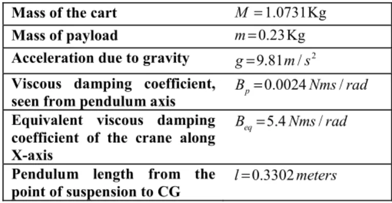
The two-dimensional single pendulum gantry crane system with its payload considered in this work is shown in the Fig.1. The payload is suspended from the point of suspension S, which denotes the centre of gravity of the cart. The downward vertical position of the payload is taken as reference position. The centre point G denotes the centre of gravity of the payload and the direction of the velocity of the payload with its components in X and Y Cartesian coordinates are represented in the Fig.1. Fx represents the force causing translational motion of the crane. The nomenclatures along with the values of the physical parameter are given in Table 1.
The dynamic model of SPGC can be found in [2,8]. Following simplification apply in this model, (i) Model does not include hoisting drive, thus rod length is fixed (ii) trolley or payload is assumed to be point mass (iii) trolley and payload assumed to move in X-Y plane and (iv) force on trolley due to pendulum swing is neglected.
2010 11th. Int. Conf. Control, Automation, Robotics and Vision Singapore, 5-8th December 2010
FIG.1: SPGC Model
The non-linear dynamic model of the gantry crane using Euler-Lagrange formulation with above simplifications yields
2 ( ) [ cos sin ] 2 cos sin x eq F B x M m x ml ml ml θ θ θ θ θ θ θ − = + + − + + (1) 2 cos sin p Bθ lθ lθ x θ g θ − = + + + (2) Assuming small sway angle θ, an approximate linear dynamic model for (1)-(2) can be represented in state space form as
( ) ( ) ( ) ( ) ( )
X t AX t Bu t
y t ==C x t + (3)
whereX t( )∈ℜ4 1× is the state vector, ( )u t ∈ℜis the control input, y t( )∈ℜ is the output of the system,
( ) [ T T T T T]
X t = xθ x θ and the matrices
A
andB
are given by0 0 1 0 0 0 0 1 0 ( ) ( ) 0 eq p eq p B mB mg A M M M B M m B M m g Ml Ml Ml ⎡ ⎤ ⎢ ⎥ ⎢ ⎥ ⎢ − − ⎥ =⎢ ⎥ ⎢ ⎥ ⎢ − + − + ⎥ ⎢ ⎥ ⎣ ⎦ 0 0 1 1 B M Ml ⎡ ⎤ ⎢ ⎥ ⎢ ⎥ ⎢ ⎥ =⎢ ⎥ ⎢ ⎥ ⎢− ⎥ ⎢ ⎥ ⎣ ⎦
In order to use delayed feedback control method, we chose to feedback the sway angle θ of the rod thus we chose
[
0 1 0 0]
C= . The pair ( , )A B is found to be controllable. III. DESIGN OF OUTPUT-DELAYED FEEDBACK CONTROLLER
(ODFC)
In this section, we explain the controller design following the technique in [11]. The control law adopted for this controller is mathematically given by
( ) [ ( ) ( )]
u t =K y t −y t−τ (4) Using (4) the closed loop system dynamics of (3) can be written as
0 1
( ) ( ) ( )
X t =A X t +A X t−τ (5) where, A0 = +A BKC and A1= −BKC.
The characteristic equation of (5) is a transcedental equation and one can write it as
0 1 s 0
sI A− −A e−τ = (6)
Equation (6) have infinite number of characteristic roots due to presence of the delay term in (5). To carry out the stability analysis of such time-delay system several appraoches have evolved in past as found in the literatures. Frequency domain techniques gives exact stability analysis and involves finding roots of (6) and are discussed in [1,9,11,12], whereas time-doamin technique do not involve actually computing roots of (6) and hence provides conservative stability results [3,7,15]. We adopt the exact stability analysis of [11] for the design of ODFC. The implementation of the technique for the stability analysis of SPGC under delayed feedback control is presented structurally in the form of algorithmic steps.
A. Algorithm:
• The characteristic equation in (6) is written in the genereic form as 0 ( , ) n ( ) l s l l sτ p s e−τ = Δ =
∑
(7) • Finding the complete root crossing structure for (7)using the Rekasius substitution for 1 1 s Ts e Ts τ − = − + term to convert it into resulting polynomial without transcedentality, which takes the form
2 0 0 n l l l b s = =
∑
(8) where, ( ,bl =b T p bl ij, ),ij p bij, ,1ij ≤i j n, ≤ being the elements ofA
andB
matrices.• We apply Rouths-Hurwitz criterion on (8), we determine set of
T
values i.e, { }Tc , by equating the element ofs
1row of Routh’s array to zero, and for each Tclvalue when the auxilliary equation (which is formed by the row preceedings
1in the Routh’s array) is solved it gives either a pair of imaginary roots (∓ωcli)or real and equal roots with opposite sign. As, we are interested only in the imaginary crossing frequencies so we ovelook those Tcl values that gives real roots. The computed values of Tcl and ωcl are placed in Table 2.• For each Tcl(or corresponding ωcl) there are infinitely many time delays { }τl , which one can obtain using
1 2[tan ( T) k ],k 0,1, 2.... τ ω π ω − = ∓ =
So, for the system in (5) one can get finite number of purely imaginary roots { },ωcl l=1, 2,3...m but infinitely many time delays i.e, { }τlk with k=0,1, 2...∞ . The computed delay values are placed in Table 3 for K=10 and K=20.
• The characteristic roots of system in (5) crosses the imaginary axis at {ωcl}values for infinitely many time-delays { },τlk that is computed as described above. The stability regions or switches are found by computing the root tendencies (RT) (or root crossing directions) at the point of corresponding delays
τ
lkby the following equation from ' 0 0 RT cl sgn Im lk cl lk n j s j j n j s j s i j p e jp e τ ω ω τ τ τ ω τ τ − = = = − = = = ⎡ ⎛ ⎞⎤ ⎢ ⎜ ⎟⎥ ⎢ ⎜ ⎟⎥ = ⎢ ⎜ ⎟⎥ ⎢ ⎜ ⎟⎥ ⎢ ⎜⎜ ⎟⎟⎥ ⎢ ⎝ ⎠⎥ ⎣ ⎦∑
∑
(9)The values of RT will be +1 or -1, if it comes out to be +1 NU increases by 2, if it is -1 it decreases by 2. The computation of NU can be done using equtaion (20) in [11].
• Now for finding the delay range (or stability switches) for the considered system, we rearrange the computed
lk
τ
values in an ascending order and check for NU by looking at the RT’s corresponding to delay values. The complete information about the stability switches for10
K= and K=20 are placed in Table 4.
• The necessary condition to be fulfilled is that at τ=0 the system must be Hurwitz.
Remark 1: The advantage of this technique is that it can
deal with system having commensurate delay also, but method expalined in [1] cannot handle case of commensuarte delay.
IV. SIMULATION RESULTS
The closed loop simulation for the system in (3) is carried using MATLAB for several values of time-delays and for a given gain. The initial condition for all the simulation is taken to bex(0)=
[
0 1.5 0 0]
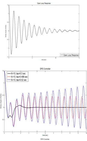
T. The open loop simulation for the sway angle is shown in Fig.2.Fig.3 shows the output response for the SPGC under ODFC withK =10. Three different delay values are considered in the first stability region i.e, 0<
τ
<0.498, (i) τ=0.3 [0,0.489)∈ for which the system is stable (ii)τ =0.489 , the system ismarginally stable and (iii)τ=0.52 [0.49,1.0046)∈ , the system is unstable. Fig.4 shows the response of the system for the stability region between 1.0046<
τ
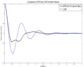
<1.2240.Fig.5 shows the comparison of the output response between LQR and ODFC. The Qmatrix for the LQR controller is chosen to be I4 4× andR=1, the LQR optimal gain obtained for the system isK=
[
1 −2.6147 0.3502 −0.6324]
. For ODFC design, the controller parameter is chosen to be K=10,τ=0.3sec , thus the control law is ( ) 10[ ( )u t = θ t −θ(t−0.3)].TABLE 1: PHYSICAL PARAMETERS OF SPGC
Mass of the cart M =1.0731Kg
Mass of payload m=0.23Kg
Acceleration due to gravity g=9.81 /m s2
Viscous damping coefficient,
seen from pendulum axis Bp=0.0024Nms rad/
Equivalent viscous damping coefficient of the crane along X-axis
5.4 /
eq
B = Nms rad
Pendulum length from the
point of suspension to CG l=0.3302meters
TABLE 2: TclAND ωclVALUES FOR VARIOUS GAINS.
K = 10 K = 20 cl T ωcl Tcl ωcl 1 0.0169 c T = − ω =c1 6.0511 Tc1 = −0.0081 ω =c1 6.0272 2 0.1739 c T = − ω =c2 8.6491 Tc2 = −0.1889 ω =c2 11.7105
TABLE 3: DELAY VALUES FOR GIVEN TclAND ωcl
K =10 K =20 1 6.0511 c ω = 1 0.0169 c T = − 2 8.6491 c ω = 2 0.1739 c T = − 1 6.0272 c ω = 1 0.0081 c T = − 2 11.7105 c ω = 2 0.1889 c T = − 0 l
τ
1.0046 0 lτ
0.498 0 lτ
1.0266 0 lτ
0.35430 1 lτ
2.0428 1 lτ
1.224 1 lτ
2.0694τ
l1 0.90849 2 lτ
3.0811 2 lτ
1.950 2 lτ
3.1122 2 lτ
1.42679 : : : : : : : : lτ
∞τ
1∞τ
l∞τ
2∞τ
l∞τ
1∞τ
l∞τ
2∞Remark 2: There is no crossing frequency corresponding to Tc3= −0.2265 for K=10 and Tc3 = −0.2237for K=20,
as it yields real and equal roots of opposite sign and hence neglected.
Remark 3: We observe from Table 4 the system is stable
in the range and again for 1.0046<
τ
<1.2240. Afterτ
=1.95 the system becomes unstable and the stability is never regained. Similarly from Table 5 the system is stable in the range 0<τ
<0.3543, atτ
=0.3543 the system becomes marginally stable and forτ
>0.3543 the system becomes unstable.TABLE 4: STABILITY SWITCHES (OR REGIONS)
K=10 Critical Time Delay lk
τ
(sec) Imaginary Roots (s= ±ωcki), clω
Root Tendency RT Number of Unstable Roots (NU) S-NU=0 0.4980 8.6491 +1 U-NU=2 1.0046 6.0511 -1 S-NU=0 1.2240 8.6491 +1 U-NU=2 1.9500 8.6491 +1 U-NU=4 2.0428 6.0511 -1 U-NU=2 2.6770 8.6491 +1 U-NU=4TABLE 5: STABILITY SWITCHES (OR REGIONS)
K=20 Critical Time Delay cl
τ
Imaginary Roots (s= ±ωcli), clω
Root Tendency RT Number of Unstable Roots (NU) S-NU=0 0.3543 11.7105 +1 U-NU=2 0.90849 11.7105 +1 U-NU=4 1.0266 6.0272 -1 U-NU=2 1.46279 11.7105 +1 U-NU=4FIG. 2: OPEN LOOP SIMULATION OF SPGC SYSTEM
FIG. 3: SWAY ANGLE FORK=10, (I)τ =0.3 [0,0.498)∈ , (II) 0.498
τ= AND (III)τ=0.52 0.498> .
FIG. 4: SWAY ANGLE FORK=10, (I)τ =1.14 [1.0046,1.224)∈ , (II) 1.224
FIG. 5: COMPARISON BETWEEN LQR & ODFC WITH K=10 AND 0.3sec
τ= .
V. CONCLUSIONS
In this work, implementation of the ODFC design for controlling the sway angle of the linearized SPGC system using the exact stability analysis in [11] is presented for the first time. This analysis allowed us to find out the stability region for different delay ranges with a pre-selected value of controller gain. The method of finding stability switches for time-delay system using this method is much more convenient and structured than that presented in [1] and references there in.
One can observe that the stability regions determined using the analysis for a given gain matches exactly with the simulation results as shown in FIG.3 and 4. The stability region reduces gradually as the value of gain is increased, this fact can be observed by comparing the regions obtained for
10
K= and K=20 in Table 4 and 5 respectively. The ODFC design is compared with the LQR and found that the former one is superior in terms of quality of transient response. The implementation of this ODFC is much simpler as we need to feed back only one state information, while in case of LQR we are to feed back all the four states thus needing four sensors.
ACKNOWLEDGMENT
This project work is supported by AICTE. Govt. of India under research promotion scheme, vide grant no. 8023/BOR/RID/RPS-229/2008-2009.
REFERENCES
[1] A. Jnifene, “Active vibrational control of flexible structure using delayed position feedback,” System and control letters, Vol 56, pp. 215-222, 2007.
[2] D.Liu,J.Yi,D.Zhao,W.Wang, “Swing free transporting of two-dimensional overhead crane using sliding mode Fuzzy control,” Proceedings of American Control Conf., Boston, 1764-1768, 2004.
[3] J.P Richard, “Time-delay systems: An overview of some recent problems”, Automatica, Vol 39, pp. 1667-1694, 2003.
[4] J.M. Hyde,W.P.Seering, “Using input command pre-shaping to supress multiple mode vibration,” IEEE Int. Conf. on Robotics and Automation, Sacramento, CA, Vol 3, pp. 2604-2609, 1991.
[5] J.E Marshall, Control of Time delay system. Stevenage, U.K: Peter Peregrinus, 1979.
[6] K. V. Singh, B.N. Datta, M. Tayagi, “ Zero assignment in vibration: with or without time-delay,” Proceedings of ASME IDETC/CIE, Las Vegas, NV, Sep. 2007.
[7] K. Gu, V.L Kharitonov, J.Chen, Stability of time-delayed system, Boston, Birkhauser, 2000.
[8] Md. A. Ahmad, “Active sway suppression techniques of gantry crane system”, European Journal of Scientific Research, Vol 27, No. 4, pp. 322-333, 2009.
[9] M. Ramesh, S. Narayana, “Controlling Chaotic motions ina two dimensional airfoil using time-delay feedback”, J. Sound Vibration, Vol. 239, No. 5, pp. 1037-1049, 2001.
[10] M. Bodson, “Experimental comparison of two input shaping method for control of resonant system”, IFAC world congress, San Francisco, CA, 1996.
[11] N. Olgac, R. Sipahi, “An eaxct method for stability analysis of time-delayed linear time-invariant system”, IEEE Transc. On Automatic Control, Vol. 47, No. 5, pp. 793-797, May 2002.
[12] N. Olgac, R. Sipahi, “A new practical stability analysis method for time-delayed LTI system, 3rd IFAC workshop on TDS (TDS 2001), Santa Fe, December 2001.
[13] R.Dey, G.Ray, S.Ghosh, A. Rakshit, “Stability analysis for continous system with additive time-varying delay: A less conservative result”, Appl. Mathem. Comput., Vol. 215, pp. 3740-3745, 2010.
[14] R. Dey, S.Ghosh, G.Ray, “Delay-dependent stability analysis of linear system with multiple state delays”, 2nd IEEE,ICIIS, Srilanka, pp. 255-260, 2007.
[15] S. Xu, J. Lam, “A survey of Linear matrix inequality techniques in stability analysis of delayed system”, Int. J. of System Science, Vol. 39, No. 12, 00. 1095-1113, Dec 2008.