Random Effects, Fixed Effects and Hausman’s Test for the Generalized Mixed Regressive Spatial Autoregressive Panel

Syracuse University

Syracuse University

SURFACE

SURFACE

Center for Policy Research

Maxwell School of Citizenship and Public

_Affairs

Fall 12-2014

Random Effects, Fixed Effects and Hausman’s Test for the

Random Effects, Fixed Effects and Hausman’s Test for the

Generalized Mixed Regressive Spatial Autoregressive Panel

Generalized Mixed Regressive Spatial Autoregressive Panel

Badi Baltagi

Syracuse University, [email protected]

Long Liu

University of Texas at San Antonio, [email protected]

Follow this and additional works at: https://surface.syr.edu/cpr

Part of the Econometrics Commons, and the Economic Theory Commons

Recommended Citation

Recommended Citation

Baltagi, Badi and Liu, Long, "Random Effects, Fixed Effects and Hausman’s Test for the Generalized Mixed Regressive Spatial Autoregressive Panel" (2014). Center for Policy Research. 207.

https://surface.syr.edu/cpr/207

This Working Paper is brought to you for free and open access by the Maxwell School of Citizenship and Public Affairs at SURFACE. It has been accepted for inclusion in Center for Policy Research by an authorized administrator

Random Effects, Fixed Effects

and Hausman’s Test for the

Generalized Mixed Regressive

Spatial Autoregressive Panel

Badi H. Baltagi and Long Liu

__________

CENTER FOR POLICY RESEARCH – Fall 2014

Leonard M. Lopoo, Director

Associate Professor of Public Administration and International Affairs (PAIA)

Associate Directors

Margaret Austin Associate Director Budget and Administration

John Yinger

Trustee Professor of Economics and PAIA Associate Director, Metropolitan Studies Program

SENIOR RESEARCH ASSOCIATES

Badi H. Baltagi... Economics Robert Bifulco ... PAIA Thomas Dennison ... PAIA Alfonso Flores-Lagunes ... Economics Sarah Hamersma ...PAIA William C. Horrace ... Economics Yilin Hou ...PAIA Duke Kao... Economics Sharon Kioko ... PAIA Jeffrey Kubik... Economics Yoonseok Lee ... Economics Amy Lutz... Sociology Yingyi Ma... Sociology Jerry Miner... Economics

Cynthia Morrow ... PAIA Jan Ondrich...Economics John Palmer... PAIA Eleonora Patacchini ...Economics David Popp ... PAIA Stuart Rosenthal ...Economics Ross Rubenstein... PAIA Rebecca Schewe ...Sociology Amy Ellen Schwartz ... PAIA/Economics Perry Singleton………...Economics Abbey Steele... PAIA Michael Wasylenko ... ……….Economics Peter Wilcoxen...…PAIA

GRADUATE ASSOCIATES

Christian Buerger ... PAIA Emily Cardon ... PAIA Hannah Dalager ... PAIA Maidel De La Cruz... PAIA Carlos Diaz ...Economics Vantiel Elizabeth Duncan ... PAIA Alex Falevich ...Economics Lincoln Groves ... PAIA Ruby Jennings... PAIA Yusun Kim ... PAIA Bridget Lenkiewicz ... PAIA Michelle Lofton ... PAIA

Roberto Martinez ...PAIA Qing Miao ... PAIA Nuno Abreu Faro E Mota... Economics Judson Murchie ...PAIA Sun Jung Oh ... Social Science Brian Ohl ...PAIA Laura Rodriquez-Ortiz ...PAIA Timothy Smilnak ... PAIA Kelly Stevens ...PAIA Rebecca Wang ... Sociology Pengju Zhang ... Economics Xirui Zhang ... Economics

STAFF

Kelly Bogart...….………...….Administrative Specialist Karen Cimilluca...….….………..…..Office Coordinator Kathleen Nasto...Administrative Assistant

Mary Santy..….…….….……....Administrative Assistant Katrina Wingle...….……..….Administrative Assistant

Abstract

This paper suggests random and fixed effects spatial two-stage least squares estimators

for the generalized mixed regressive spatial autoregressive panel data model. This extends the

generalized spatial panel model of Baltagi, Egger and Pfaffermayr (2013) by the inclusion of a

spatial lag dependent variable. The estimation method utilizes the Generalized Moments method

suggested by Kapoor, Kelejian, and Prucha (2007) for a spatial autoregressive panel data model.

We derive the asymptotic distributions of these estimators and suggest a Hausman test a la Mutl

and Pfaffermayr (2011) based on the difference between these estimators. Monte Carlo

experiments are performed to investigate the performance of these estimators as well as the

corresponding Hausman test.

JEL No.

C12, C13, C23

Keywords:

Panel Data; Fixed Effects; Random Effects; Spatial Model; Hausman Test

Address correspondence to: Badi H. Baltagi, Center for Policy Research, 426 Eggers Hall,

Syracuse University, Syracuse, NY 13244-1020; e-mail: [email protected].

Long L

iu: Department of Economics, College of Business, University of Texas at San Antonio,

One UTSA Circle, TX 78249-0633; e-mail: [email protected].

Random

E¤ects,

Fixed

E¤ects

and

Hausman’s

Test

for

the

Generalized

Mixed

Regressive

Spatial

Autoregressive

Panel

Data

Model

Badi

H.

Baltagi

_,

_Long

_Liu

November

1,

2014

Abstract

Thispaper suggests randomand …xede¤ects spatialtwo-stageleastsquares estimators for thethe generalizedmixedregressivespatialautoregressivepaneldatamodel. Thisextendsthegeneralizedspatial panelmodelofBaltagi,EggerandPfa¤ermayr(2013)bytheinclusionofaspatiallagdependentvariable. The estimationmethod utilizes theGeneralizedMoments method suggestedby Kapoor, Kelejian,and Prucha(2007)for aspatialautoregressivepaneldatamodel. Wederivetheasymptoticdistributions of theseestimatorsand suggestaHausman testalaMutl andPfa¤ermayr(2011)basedonthedi¤erence between these estimators. Monte Carlo experimentsare performed to investigate the performance of theseestimatorsaswellasthecorrespondingHausmantest.

KeyWords: PanelData; FixedE¤ ects;Random E¤ ects;SpatialModel;Hausman Test.

JELclassi…cation: C12;C13;C23

1

Introduction

Anselin(1988)andKapoor,Kelejian,andPrucha(2007)consideredtwodi¤erentvariantsofarandome¤ects panel data model with spatially correlated errors. The …rst paper estimated it with maximum likelihood methods and the second estimated it with a generalized moments (GM) method that is computationally simpler. Baltagi, EggerandPfa¤ermayr(2013)generalizedthisrandome¤ects spatialmodel toencompass bothcasesandderivedLMandLRteststodistinguishbetweenthesemodels. Thegeneralizedmodelallows the individual e¤ects and theremainder errors to have di¤erent spatial autoregressive parameters. Using maximumlikelihood methods,Baltagi, EggerandPfa¤ermayr(2008)examinedthe consequencesof model misspeci…cation in this context using MonteCarlo simulations. These papers assume that the underlying

_{We would like to thank the editor Essie Maasoumi, an Associate editor and two anonymous referees for their helpful} comments and suggestions. Long Liu gratefully acknowledges the summer research grant from the College of Business at UTSA.

y_{Addresscorrespondenceto: BadiH.Baltagi, CenterforPolicyResearch,426EggersHall,SyracuseUniversity,Syracuse,} NY13244-1020;e-mail: [email protected].

z_{Long Liu: Department of Economics, College of Business,University of Texasat San Antonio, One UTSACircle, TX} 78249-0633;e-mail: [email protected].

spatial panel model is random e¤ ects (RE). Spatial panel data model with …xed-e¤ ects (FE) have been considered by Baltagi and Li (2006), Mutl and Pfa¤ermayr (2011), and Lee and Yu (2010)to mention a few. In fact, Baltagi and Li (2006) obtained the maximum likelihood estimator of a …rst order spatial autoregressivemodel with …xed e¤ects and usedit to forecast theconsumption of liquoracross a panel of US states, while Leeand Yu (2010)established the asymptotic properties of a quasi-maximum likelihood (QML) estimatorfor thespatial paneldata model with …xed-e¤ects. However, as pointedoutby Kapoor, Kelejian,andPrucha(2007),hereafterdenotedby(KKP),theQMLestimationofCli¤andOrd(1973,1981) type models entail substantial computational problems if thenumber of cross sectionalunits is large. To circumvent thesecomputational problemsforthemixed regressive spatialautoregressive(MRSAR)model, MutlandPfa¤ermayr(2011)suggesteda…xede¤ectstwo-stageleastsquares(FE-2SLS)estimatorbasedon a generalized moments(GM) estimator a la Kapoor, Kelejian, and Prucha (2007) extending the latter to include a spatiallag ofthedependent variable. Mutland Pfa¤ermayr(2011)alsopropose aHausman test basedonthedi¤erencebetweenthe…xedandrandome¤ectsspeci…cationofthismodel. Thispaperapplies theFE-S2SLSestimatorofMutlandPfa¤ermayr(2011)tothegeneralizederrorcomponentmodelconsidered byBaltagi, Eggerand Pfa¤ermayr(2013)by addinga spatial lag term. Wealso suggest a random e¤ects spatial two-stage least squares (RE-S2SLS) estimator using GM estimation of this generalized MRSAR error component model. Following Mutl and Pfa¤ermayr (2011), we apply a Hausman test based on the di¤erence between the …xed and random e¤ects speci…cation of this generalized MRSAR model. Small sample properties of these estimators as well as the size of the proposed Hausman test are studied using Monte Carlo experiments. We show that a misspeci…ed GM estimator can cause substantial loss in root meansquarederror(RMSE)andwrongsize forthecorrespondingHausmantest.

Therestofthepaperisorganizedasfollows. Section2introducestheRE-S2SLSandFE-S2SLSestimators for the MRSAR model. Generalizedmoments (GM) estimators a laKapoor, Kelejianand Prucha (2007) areproposedforthismodelandtheirasymptoticdistributionsarederived. FollowingMutlandPfa¤ermayr (2011),a Hausmantest isproposedbasedonthedi¤erence betweentheFE-S2SLSandfeasibleRE-S2SLS estimatorsofthisspatialpanelmodel. Simulationresultsarereportedinsection3,whilesection4concludes thepaper. AllproofsarerelegatedtotheAppendix.

2

The

MRSAR

Model

LetusconsidertheMRSARmodelwhichisbasedonageneralizedspatial errorcomponentsmodel studied inBaltagi,EggerandPfa¤ermayr(2013)butextendsitbyaddingaspatiallagofthedependentvariableas

in MutlandPfa¤ermayr(2011). Foreachtime periodt= 1;:::;T,thedata aregeneratedaccording tothe followingmodel:

yN(t) = MNyN (t) +XN(t)+uN (t) (1)

uN(t) = u1N +u2N(t); (2)

u1N = 1WNu1N+N; (3)

u2N(t) = 2WNu2N(t) +N (t); (4)

whereyN (t)denotestheN1vectorofobservationsonthedependentvariableinperiodt. XN (t)denotes

the N K matrix of observations on exogenous regressors in period t, which may contain the constant term. is thecorresponding K1 vector ofregression parameters, and uN (t) denotes theN1 vector

ofdisturbanceterms. uN (t)followsanerrorcomponentmodel whichinvolvesthesumoftwodisturbances.

TheN1 vectoru1N capturesthetime-invariantunit-speci…ce¤ectsand thereforehasnotime subscript.

TheN1vectoroftheremainderdisturbancesu2N(t)varieswithtime. Bothu1N andu2N (t)arespatially

correlatedwith thesame spatialweights matrixWN, but withdi¤erentspatial autocorrelation parameters

₁and₂,respectively. BothMN andWN areNN weightingmatricesofknownconstantswhichdonot

vary over time. MN and WN may or may notbe the same. This generalizesthe model in Baltagi, Egger

andPfa¤ermayr(2013)byincorporatingaspatiallagtermMNyN (t).

Stackingthecross-sectionsovertimeyields

yN = MNyN +XN+uN (5) uN = Zu1N +u2N; (6) u1N = 1WNu1N+N; (7) u2N = 2(IT WN )u2N+N; (8) 0 0 N(T)]0, uN = [u0N(1); : : : ; u0N(T)]0, u2N = 0 N 0N(T)] XN = [XN0 where yN = [y (1); : : : ; y , (1); : : : ; X 0 0

[u0_2N(1); : : : ; u0_2N(T)] and vN = [v_N0 (1); : : : ; v0_N(T)]. The unit-speci…c errors u1N are repeated in all

timeperiods usingtheN T N selectormatrixZ =T IN,where T isavectorof onesofdimensionT

andIN isanidentitymatrixofdimensionN,seeBaltagi(2013). Let i;N andfit;Ngdenotetheelements

oftheN 1vector ofindividuale¤ects _N andthen1vectorof remainderdisturbancesN. Following

Kapoor,KelejianandPrucha(2007),weemploythefollowingassumptions:

Assumption1 Let T be a …xed positive integer. (a) Forall 1 tT and 1i N, N 1 the error components it;N are identically distributedwith zero mean and variance 2, 0< 2 < bv <1,and …nite

fourth moments. In addition, for each N 1 and 1 t T, 1 i N the error components it;N are independently distributed. (b) For all 1 i N, N 1; the unit speci…c error components i;N are independently distributedwith zero mean and variance 2

,0 < 2 < b <1, and …nite fourth moments. In addition, for each N 1; and 1 i N the unit speci…c error components _i;N are independently

distributed. (c) Theprocesses _i;N and_fit;Ng areindependent.

Assumption2 (a) Alldiagonal elements ofMN andWN arezero. (b) jj<1,j1j<1 andj2j<1. (c) The matricesIN �MN,IN �1WN andIN�2WN are nonsingular. Therow andcolumnsums of MN,

�1 �1 �1

WN,(IN�MN ) ,(IN �1WN ) and(IN �2WN ) are boundeduniformly inabsolutevalues forall

j_j<1,_j1j<1 and_j2j<1.

As pointedoutbyBaltagi,EggerandPfa¤ermayr(2013),thismodel nestsvarious spatialpanelmodels in theliterature. For example, for the casewhere there is no spatial lag, i.e., = 0; and when ₁ =₂, thisreduces tothespatial randome¤ects modelconsidered inKapoor, Kelejianand Prucha(2007). When = 0and 1 = 0, itreduces totheAnselin(1988)spatialrandome¤ects modelalso describedin Baltagi,

SongandKoh(2003)andAnselin,LeGalloandJayet(2008). When1=2= 0,itreducestothefamiliar

random e¤ects (RE) panel data model with no spatial e¤ects, see Baltagi (2013). In the presence of the spatiallagofthedependentvariable,itneststheMRSARmodelconsideredbyMutlandPfa¤ermayr(2011) andDebarsyand Ertur(2010),tomentiona few.

2.1

The

RE-S2SLS

Estimator

Asshownin KelejianandPrucha(1998)forthecross-sectioncase,thespatiallagMNyN iscorrelatedwith

thevectorofdisturbancesuN. Therefore,theOrdinary LeastSquares(OLS)estimatorwillbeinconsistent.

� 0

De…neZN = (MNyN; XN)and= ;0 . Withthis notation,theMRSARmodel canbe rewrittenas

yN =ZN+uN: (9)

For the cross-sectionspatial autoregressive model, Kelejianand Prucha (1998)suggested instruments like

�

= XN; MNXN; M2 . De…ne =var(uN ). Asshownin Baltagi,EggerandPfa¤ermayr(2013),

HN NXN u

h i�1

�1 �1 �1

=JT T 2(A0A) +2(B0B) +�2[ET (B0B)]; (10)

u

where A =IN �1WN and B =IN �2WN. ET =IT �JT, JT =JT=T and JT is a matrix of ones of �1=2

dimensionT. Multiplying Equation(9)by u ,weget

�1=2 �1=2 �1=2

� � �

De…neP =JT IN andQ=IN T�P,whereIN T isanidentitymatrixofdimensionN T.FollowingBaltagi �1=2

and Liu (2011), we apply the instruments u HN with HN = (QHN; P HN ) to this transformed panel

autoregressivespatialmodel. Therandome¤ectsspatialtwo-stageleastsquaresestimator(RE-S2SLS)of isgivenby

h i�1

�1 _�1 �1

RE�S2SLS

withvariancevar

b _Z0 �1_H N N HN0 �1HN HN0 ZN ZN0 �1HN HN0 �1HN HN0 u�1yN (12) = _{u u u u u} RE�S2SLS h b i�1 �1 Z0 �1_{H H}0 �1_H N N N N HN0 �1ZN = _{u u u} .

Kapoor,KelejianandPrucha(2007)consideredthespecialcasewhere = 0and₁=₂ andproposed GMestimators of₂and2 _{basedonthefollowingthreemomentconditions:}

1 E[0NQN ] = 2; (13) N(T_�1) 1 _E[ 2tr(WN0 WN ) N 0 _Q N ] = ; (14) N(T_�1) N 1 E[0_NQN ] = 0; (15) N(T_�1)

where N = (IT WN )N. De…ne u2N = (IT WN )u2N and u2N = (IT WN ) u2N. Substitute N =

u2N�2u2N andN =u2N�2u2N into thesystemofequationsgivenabove,weget

1 ₀ 2 ₀ 1 2 0 2 E[u_2NQu2N ]� 2E[u2NQu2N] + 2E[u2NQu2N ] = ; (16) N(T _�1) N(T_�1) N(T_�1) 1 2 1 2_tr(W0 _{WN )} 0 0 2 0 N E[u_2NQu2N ]� 2E[u2NQu2N] + 2E[u2NQu2N ] = (17); N(T_�1) N(T_�1) N(T_�1) N 1 ₀ 1 _{0 0} 1 ₀ E[u_2NQu2N ]� 2E[u2NQu2N + u2NQu2N] + 22E[u2NQu2N ] = 0: (18) N(T_�1) N(T_�1) N(T_�1) 0

Note that Q(T u1N ) = 0. Therefore, for the general model in Equations (5)-(8), we have u QuN N =

0 0 0 0 0

u2NQu2N; uNQuN =u2NQu2N anduNQuN =u2NQu2N. Thissystemcanbeexpressedas

0 �0_{N 2}; 2₂; 2 _�0_N = 0; (19) 1 0 2 _{E[u Qu0} 1 ₀ N] � E[u QuN ] 1 N(T�1) N N(T�1) N B B B @ C C C A where�0 N = N(T2�1)E[u Qu0N N] �N(T1�1)E[u Qu0N N ] N1tr(WN0 WN ) 1 1 _{E[u Qu0 0} 1 ₀ N + u QuN ] � E[u Qu N ] 0 N N N N(T�1) N(T�1) 0 1 _E[u0 _Qu N ] N(T�1) N B B B @ C C C A. and0_N = 1 _E[u0 _Qu N ]

N LetubN denote the2SLS residualsfrom(5) ignoringtherandom e¤ects, N(T�1)

1

h i�1 �1 _{0 0} �1 0 0 0 i.e.,u_bN =yN�ZNb2SLS,whereb2SLS N0 yN. 0

andg bethesampleanaloguesof�0 _and0 _{substitutingub}

N foruN:WecangetaGMestimatorbysolving

N N N � 0 ~₂; ~2 =argmin N0 ₂; 2 0N ₂; 2 ; ₂₂[_�a0; a0]; 22[0; b0] ; (20) � 0 1 where0 ₂; 2 _=G0 2; 22; 2 �gN,a01andb0bv. N N LetGN Z HN(H HN ) H ZN Z HN (H HN ) H = _{N N N N N}

Assumption3 The smallest eigenvaluesof�0

N�N areboundedaway fromzero.

Kapoor, Kelejian and Prucha (2007)showed that, for their model with no spatial lag, and where the disturbances are replaced by OLS residuals, ~ and ~2 are consistent. It is worth pointing out that the condition Q(T u1) = 0 holds for thegeneral model given in equation (5), and not only for thespecial

caseinKapoor, KelejianandPrucha (2007). Therefore,forallvaluesof1 and2 intheparameter space,

theGM estimatorof₂ and2 _{suggestedbyKapoor,KelejianandPrucha(2007)andappliedtoourmodel}

based on 2SLS residuals, will also be consistent. By Theorem 1 of Kapoor, Kelejian and Prucha (2007),

� �

2 p

we have ~₂;~ _{! 2}; 2 _{under assumptions1-3 as N ! 1. Similarly, we introduce thefollowing GM}

estimatorsof₁ and2 :

De…ne =WN. Wehavethefollowingthreemomentconditions:

1 N 0 E[_NN] 0 2; (21) NWN ); = 1 N 1 2tr(W 0 E[_NN] = (22) N 1 N 0 E[_NN] = 0: (23)

Similarlyde…neu1N =WNu1N andu1N =WNu1N. SubstituteN =u1N �1u1N andN =u1N �1u1N

intothesystemofequationsgiven above,weget

1 N 2 N 1 2₁E[ 0 E[u_1Nu1N ]� 1E[u01Nu1N ] + u0 0 2; (24) NWN ); 1Nu1N] = N 2 1 ₀ 2 1 1 0 ₁E[u 2₁E[u0 (25) 0 1Nu1N ]� E[u _1Nu1N ] + 1Nu1N] = tr(W N N N N 1 N 1 2₁E[ 0 E[u_1Nu1N ]� 1E[u1Nu1N + u10Nu1N ] + u01Nu1N] = 0: (26) N N

Thissystemcanbeexpressedas

0

0 1 2_E[u0 _�1_E[u0 ₁ B N 1Nu1N ] _N 1Nu1N ] C B 2 0 _�1 0 1 C where�1 ₌ B E[u E[u tr(W0 _C N _N 1Nu1N ] _N 1Nu1N ] _N NWN) @ A 1_E[u0 0 _�1 0 1Nu1N + u u1N ] E[u u1N ] 0 N 1N N 1N 0 1 1_E[u0 1Nu1N ] N B C B C 1 1 and1 ₌

B1_E[u0 _{C. De…ne S=P� Q=ST IN,whereST =JT� ET. Also}

N _@N 1Nu1N ]_A T�1 T�1 1_E[u0 1Nu1N ] N 1 ₀ � 0 � Wk Wl = u IT S IT uN '_kl;N N T N N N � 0 � 0 = _{N T}1 uN IT WNk (ST IN ) IT WNl uN 1 ₀ � Wk0 = _{N T}uN ST NWNl uN fork;l= 0;1;2. Hence � 1 ₀ � Wk0 E '_kl;N = E u_N ST NWNl uN N T 1 ₀� Wk0 = E (Zu1N+u2N ) ST NWNl (Zu1N+u2N ) N T ₀� � Wk0 0 Wk0 = 1 E (Zu1N ) ST NWl (Zu1N ) + 1 E u ST NWl u2N N 2N N N T N T 2 ₀ � Wk0 + E u2N ST NWNl Zu1N N T I+II+III: Notethat 1 ₀� 1 � 1 � Wk0 0 Wk0 0 I= E (Zu1N ) ST NWNl (Zu1N ) = E u1N 0TSTT NWNl u1N = E u1NWNk0WNl u1N N T N T N 1 1 since0 _S TT =0 JT � ET T =0 JTT � 0 ETT =T usingJTT =T andETT =0; T T T�1 T T�1 T h i 1 ₀ � 1 � 0� � Wk0 0 B�1 Wk0 B�1 II = _{N T}E u2N ST NWNl u2N = _{N T}E N IT ST NWNl IT N 1 � = E _N0 ST B�10W_Nk0W_NlB�1 N N T 1 � = _{N T}2vtr(ST )tr B�10WNk0WNlB�1 = 0 1 sincetr(ST ) =tr JT �_T�1ET = 0;and 2 ₀ � Wk0 III =_{N T}E u2N ST NWNl Zu1N = 0

� � � � � � � � � � � = _N1E u0 W_Nk0 0 W1Nlu1N SuN] sinceu₀1N B B B @

andu2N areindependentbyAssumption1. Hence,one getsE

0 1 0 1 1 0 '_{kl;N 1N} ; 2 N TE[u SuN N ] N TE[u SuN N ] 1 N TE[uN WN ) C C C A; and 1 N = B B B @ C C C A �1 N = _{N T}2 E[u Su0N N ] N T1 E[u SuN0 N ] N1tr(WN0 _{N T}1 E[u SuN0 N] . The 1 N T 1 N T 1 N T 0 0 0 0 N E[u Su N+ u SuN ] E[u SuN ] 0 E[u SuN] 0 N N N 1 2 _{u~0 Su~} 1 ₀ N � u~ Su~N 1 N T N N T N B B B @ C C C A

sampleanaloguesto�1 _and1 _areG1

N N N N T2 ~0 1 _{~0 ~} 1 ~ tr(W0 N and S S WN ) = uN uN N TuN uN N 1 _u~0 _Su~ 0 1 _~0 N +u~ Su~N � u Su~N 0 N T N N N T N 1 0 1 _u~0 _Su~ N N T N B B B @ C C C A

1 1 _u~0 _{Su~ ,respectively. Hence,aGM estimatorcan beobtainedfrom} N g_N = _N N T 1 _u~0 _Su~ N N N T 2 ; ₁ 1 �g_N,a11andb1b. 0 1_{N 1}; 2 1_N 2 ₁;~ =argmin ; ₁₂[_�a1; a1]; 2 2[0; b1] ; (28) ~ 0 where1_{N 1}; 2 _=G1 1; 21; 2 N p ! ~ 2 ₁;~ ₁; 2

Theorem 1 Under Assumptions1-3,wehave asN_{! 1}.

WiththeGMestimatorsof~₁,~₂,~2and~2,thecorrespondingrandome¤ectsfeasiblespatialtwo-stage leastsquaresestimatorbRE�F S2SLS isgivenby

_�1 �1 _�1 RE�F S2SLS where b = ZN0 ~u�1HN HN0~u�1HN HN0~u�1ZN ZN0 ~u�1HN HN0~u�1HN HN0~�u1yN; (29) _{�1 �1}�1 _{h i} ~�1_=J 2 _A~0~ 2 _B~0~ �2 _B~0~ T T~ A + ~ B + ~ ET B : (30) u Assumption4 XN h

isnon-stochastic. The elements of XN

1 _{H0 J}

T T 2(A0A) N

are boundeduniformlyin absolutevalue.

Fur-i�1

�1 �1

+2 (B0B)

thermore,the limit0= lim _{N T} HN,

N!1 h i�1 �1 �1 +2 1 _H0 _[E 1 T (B0B)]HN, �0 = lim H0 JT T 2(A0A) N N T N (B0B) ZN and 1 = lim N!1N T N!1 1 _H0

�1= lim N T N[ET (B0B)]ZN are…nite andnonsingular. N!1

Thetheorembelowestablishesconsistencyandasymptoticnormalityoftherandome¤ectsfeasiblespatial two-stageleastsquaresestimator. Theproofofthetheoremisgivenin theappendix.

_�1 p d !N bRE�F S2SLS� asN _{! 1}. �₀00�1�0 +�2�01�11 �1

Next,weturntothespecialcasesofthisgeneralmodel. UndertheKKPmodel,butnowwitha spatial lag,wehave 1=2, andasaresultA=B,andEquation(10)reducesto

�

�1₌ 2_J

T +�2ET (B0B); (31)

u 1

where2

1=T 2+2. Kapoor, KelejianandPrucha(2007)suggestestimating21by

~ =12 _N1 (~uN�~2WNu~N )0Q(~uN �~2WNu~N ):

Inthiscase,theasymptoticdistributionofthecorrespondingbRE�F S2SLS isthesameasinTheorem2with

1 _H0 1 _H0

0 and�0 reducingto 0= lim _{N T} N 12JT (B0B) HN, and�0= lim N T N 12JT (B0B) ZN,

N!1 N!1

respectively.

Under theAnselinmodel,butnowwitha spatiallag,wehave ₁= 0and henceA=IN. Equation(10)

reducesto h i�1 �1_{= T} 2_I N+2(B0B) +�2[ET (B0B)]: (32) u JT �1 Wecanestimate2

fromthe…rstEquationin (21)as

1 ₀ 1 ₀ 1 ₀

2

~ = u~NSu~N = u~NP u~N � u~NQu~N:

N T N T N T(T_�1)

Note that it is the same estimator of 2

for the random e¤ect model with 1 = 2 = 0. From the p

proof of Theorem 1, we know that under Assumptions 1-3, ~2 _! 2 _{as N ! 1. With these GM}

mators of ~₂, ~2 and ~2, we obtain the random e¤ects feasible spatial two-stage least squares estimator

bRE�F S2SLS. Similarto Theorem 2,we can showthat bRE�F S2SLS hasthesame asymptotic distribution

h i�1

1 _H0 �1

asinTheorem2,with0and�0reducingto0= lim _{N T} N JT T 2IN +2(B0B) HN,and N!1

_{h i�1}

1 _H0 �1

�0= lim N T N JT T 2IN +2(B0B) ZN,respectively. N!1

2.2

The

FE-S2SLS

Estimator

Let_fu1i;NgandfXit;NgdenotetheelementsoftheN1vectorofu1N andtheN T K vectorofXN. A

criticalassumption forthe consistencyof theRE estimatoristhat E(u1i;NjXit;N ) = 0. If theunobserved

individualinvariante¤ects arecorrelatedwithXit;thenE(u1ijXit)6= 0andREisinconsistent. Aspointed

out in Lee and Yu (2010), with the …xed e¤ects speci…cation, the panel models in Baltagi, Egger and Pfa¤ermayr(2013),Kapoor,KelejianandPrucha (2007)andAnselin(1988)have thesame representation. Morespeci…cally,premultiplying equation(5)bythe…xed e¤ects(orwithin)transformationQ=ET IN,

oneobtains

sinceQ(T u1N ) = 0, see Baltagi (2013). The…xed e¤ects two-stage leastsquares estimator(FE-2SLS)

estimator

h i�1

�1 �1

b

F E�2SLS = ZN0 QHN (HN0 QHN ) HN0 QZN ZN0 QHN (HN0 QHN ) HN0 QyN (34)

wipes outthe individual e¤ects and does notrequire the estimation of ₁ or 2

. However, this estimator

ignoresthespatialautocorrelationintheerror. Togaine¢ ciency,one canapplytheCochrane-Orcutttype spatialtransformationonthewithintransformedmodelinEquation(33)toobtaintheFE-S2SLSestimator assuggestedin MutlandPfa¤ermayr(2011). Morespeci…cally,wepremultiplyequation(33)byIT B;to

get

(ET B)yN = (ET B)ZN+QN: (35)

Thisusesthefactthat(IT B)Q= (ET B) =Q(IT B)and(IT B)Qu2N =Q(IT B)u2N =QN.

Applying the instruments (ET B)HN, we get the…xed e¤ects spatial two-stage least squaresestimator

(FE-S2SLS)ofgivenby n o�1 �1 bF E�S2SLS = ZN0 [ET (B0B)]HN(HN0 [ET (B0B)]HN ) HN0 [ET (B0B)]ZN (36) �1 Z0 (B0B)]HN(H0 (B0B)]HN ) H0 (B0B)]yN n o�1 N[ET N[ET N[ET Z0 �1 with var bF E�S2SLS = 2 N[ET (B0B)]HN(HN0 [ET (B0B)]HN ) HN0 [ET (B0B)]ZN . If

₂ = 0; then B =IN and theFE-S2SLS estimatorin Equation(36) reduces to theFE-2SLS estimator in

Equation(34). Usingthe GM estimators of~2 and ~2 fromEquation(20), thecorresponding …xed-e¤ects

feasiblespatial two-stage leastsquaresestimator(FE-FS2SLS)bF E�F S2SLS isobtained byreplacing B by

~

itsestimatorB =IN �~2WN, i.e.,

_{h i h i �1 h i} �1

bF E�F S2SLS = ZN0 ET B~0B~ HN HN0 ET B~0B~ HN HN0 ET B~0B~ ZN

h i h i �1 h i

Z_N0 ET B~0B~ HN HN0 ET B~0B~ HN HN0 ET B~0B~ yN: (37)

Thisestimatorcanbecomputedconvenientlyasthe…xede¤ectstwo-stageleastsquaresestimatorafter

pre-~

multiplyingthemodelinequation(5)byIT B. Thetheorembelowestablishesconsistencyandasymptotic

normalityoftheFE-FS2SLSestimators. Theproofofthetheoremisgivenin theappendix.

p d � �1

Theorem 3 UnderAssumptions1-4,wehave N T bF E�F S2SLS� !N 0; 2 �011�

1_�

1 asN !

1.

OneoftheadvantagesoftheFE-FS2SLSestimatorofisthatitdoesnotdependon2 _and

1:Hence,

theFE-FS2SLSestimatorisrobustto di¤erentvaluesof 2 _and

1. AnotheradvantageoftheFE-FS2SLS

� � �

2.3

Hausman’s

Test

Onecan performHausman’s (1978)speci…cation test forthis generalized MRSAR paneldata model. The

b

null hypothesisis H0 :E(u1i;NjXit;N ) = 0. Under H0, RE�S2SLS given in (12)isthe e¢ cientestimator,

whileunder thealternativeH1:E(u1i;NjXit;N )6= 0;bRE�S2SLS isinconsistent. Incontrast,bF E�S2SLS is

consistentunder thenullandalternative. Letq=bF E�S2SLS �bRE�S2SLS andnotethat

cov bF E�S2SLS;bRE�S2SLS 0 b b = E F E�S2SLS� RE�S2SLS� n o�1 �1 = ZN0 [ET (B0B)]HN (HN0 [ET (B0B)]HN ) HN0 [ET (B0B)]ZN �1 ₀ Z_N0 [ET (B0B)]HN (HN0 [ET (B0B)]HN ) HN0 [ET (B0B)]E(uNuN) h i�1 �1_{H H}0 �1_H�1_H0 �1 _Z0 �1_{H H}0 �1_H�1_H0 �1 u N N u N N u ZN N u N N u N N u ZN h i�1 Z0 �1H H0 �1H�1H0 �1 = _{N u N N u N N u} ZN b = var RE�S2SLS : Hence var(q) = var bF E�S2SLS�bRE�S2SLS

= var bF E�S2SLS +var bRE�S2SLS �2cov bF E�S2SLS;bRE�S2SLS

b b b

= var F E�S2SLS +var RE�S2SLS �2var RE�S2SLS

b b

= var F E�S2SLS �var RE�S2SLS :

�1

UnderH0,theHausmantestm=q0[var(q)] qhasalimiting2distributionwithdegreesoffreedomequal

to therankof var(q). Inpractice,estimates ofboth ₁ and ₂ are neededto calculate var bRE�S2SLS .

UndertheKapoor,KelejianandPrucha(2007)randome¤ectsspatialmodel,₁=₂andundertheAnselin (1988)randome¤ectsspatial model,₁= 0:OnecouldperformaHausman testbasedontheseRE-S2SLS versusFE-S2SLSestimatorsproposedinthispaper. Infact,MutlandPfa¤ermayr(2011)suggesteda Haus-mantest assuming₁=₂ fortheMRSAR paneldatamodel. Its sensitivityunder modelmisspeci…cation (say₁₆=₂)ischeckedinthefollowingsectionviaMonteCarloexperiments.

3

Monte

Carlo

Simulation

This section performs Monte Carlo experiments to study the …nite sample performance of the proposed estimators and thecorresponding SpatialHausman test. FollowingBaltagi, Egger andPfa¤ermayr (2013) butaddinga spatiallagterm,weconsiderthefollowingMRSARpanelmodel

yN =MNyN++xN +uN; (38) iid

where = 0:5, = 5 and = 0:5. xit is generated by xit = i +zit with i U[�7:5;7:5] and

iid iid

zit U[�5;5]. Theindividualspeci…ce¤ectsaredrawnfromanormaldistributionsothati N(0;20).

For the remainder error, we let 2 _{= 10 and} 2 _{= 10. This implies that the proportion of the total}

2

varianceduetotheheterogeneityoftheindividual-speci…ce¤ectsis 2

= 0:5. Thespatialweightmatrix

2

+

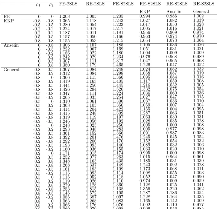
is created following Kapoor, Kelejian and Prucha (2007). The weighting matrix is referred as “3 ahead and 3 behind”. This matrix is de…ned in a circular world so that thenon-zero elements in rows1 and N are,respectively,inpositions(2;3;4; N_�2; N_�1; N)and(1;2;3; N_�3; N_�2; N_�1). Thismatrixisrow normalized so that all of its non-zero elements are equal to 1=6. In the Tables below, we reference this weightingmatrixbyJ = 6,whereJ isthenumberofnonzeroelementsin agivenrow. ₁ and₂ varyover theset_f�0:8;_�0:5;_�0:2;0;0:2;0:5;0:8_g. WeconsiderapanelwithN =100regionsandT = 5timeperiods, andweperform10,000replications. Foreachreplication,weestimatethemodelusing(i)FE-2SLSallowing for spatial lag but no spatial error correlation; (ii) RE-2SLS allowing for spatial lag but no spatial error correlation;(iii) FE-S2SLSallowingforboth spatiallag andspatial errorcorrelation;(iv)KKP RE-S2SLS allowingforbothspatial lagand errorcorrelation;(v)AnselinRE-S2SLSallowingfor bothspatial lagand errorcorrelation;(vi)GeneralRE-S2SLSallowingforbothspatial laganderrorcorrelation;and (vii)True RE-S2SLSallowingforbothspatial lagandspatialerrorcorrelation.

Table1 reportstherelativerootmeansquarederror(RMSE)ofeachestimatorof withrespecttothe true RE-S2SLS.Several conclusions emerge from this table. Not surprisingly, true RE-S2SLS is themost e¢ cientestimatorintermsofrootmeansquarederror. WhenthetruemodelisspatialRE,KKPorAnselin withaspatiallagterm,the‘correct’feasibleRE-S2SLSestimatorperformsbestandistheclosestinRMSE to the true RE-S2SLS. FE-S2SLS estimator performs much better than standard FE-2SLS which ignores the spatial correlation. For example, for ₁ = ₂ =_�0:8, therelative RMSE of FE-2SLS and FE-S2SLS with respect to trueRE-S2SLS is 1:365 and 1:243, respectively. Note that both FE-S2SLS and FE-2SLS estimators performmuch worsethan any feasiblespatial RE-S2SLSestimator. There is alsomuch gain in performing RE-S2SLS allowingfor spatial correlation than ignoring it. For ₁ = ₂ = _�0:8, the relative RMSEofRE-2SLSignoringspatialcorrelationwithrespecttotrueRE-S2SLSis1:118comparedto1:027for

theRE-S2SLSbasedonKKP. TheGeneralspatialRE-S2SLSestimatorof Baltagi,EggerandPfa¤ermayr (2013)issecondbestwithrelativeRMSEof1:039. For1= 0and2= 0:8;therelativeRMSEofRE-2SLS

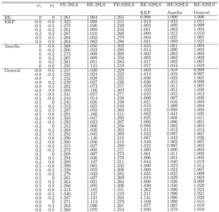
ignoring spatial correlation is 1:179 compared to 1:047 for the RE-S2SLS basedon Anselin. TheGeneral spatial RE-S2SLSestimatorisagainsecond bestwith relativeRMSE of1:052. Thegain in e¢ ciency from using the correct feasible RE-S2SLS for our experiments when the true model is a generalized MRSAR panel model with ₁ = 0:8 and ₂ = _�0:8, is as follows: The relative RMSE of the RE-S2SLS based on KKP is1:356and theRE-S2SLSbasedonAnselinis1:220,while theGeneralspatialRE-S2SLSestimator is 1:062. Table 2 reports therelative root mean squared error(RMSE) ofeach estimatorof . Similar to thesimulation resultsfor in Table1, for₁ = 0:8 and ₂ =_�0:8, Therelative RMSE of theRE-S2SLS basedonKKP is 1:262 and theRE-S2SLS basedonAnselinis 1:096,while theGeneralspatial RE-S2SLS estimatoris1:024.

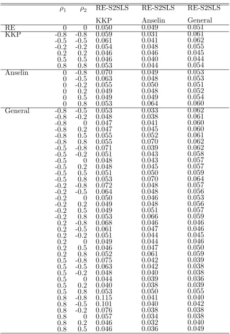
Table 3 reportstheempiricalsize (atthe5%level)of thespatialHausmantest forvarious valuesof 1

and₂ basedon10,000replications. ThisisbasedonthecontrastoftheKKPRE-S2SLSestimatorandthe FE-S2SLSin the…rst column, and the contrastof theAnselin RE-S2SLSestimator and theFE-S2SLS in thesecondcolumnandthecontrastoftheGeneralizedRE-S2SLSestimatorandtheFE-S2SLSinthethird column. Wecanseethat for₁= 0and₂=_�0:8;thespatialHausmantestbasedonKKP isover-sizedif thetruemodelis anAnselinrandome¤ects MRSARmodel. It yieldsa probabilityoftypeI errorof0:070

whenitshould be0:05. Thisoversizingof thetest getsworse when₁= 0:8 and₂=_�0:8. TheHausman testbasedonKKP yieldsatypeI errorof0:115. Incontrast,for₁=₂=_�0:8,thespatialHausmantest basedontheAnselinRE-S2SLSestimatorisunder-sizedifthetruemodelisaKKPrandome¤ectsMRSAR model. ItyieldsaprobabilityoftypeIerrorof0:031whenitshouldbe0:05. However,thisundersizingdoes notgetworse, andtheHausmantestbasedontheAnselintypeMRSARpanelmodel performs reasonably wellwhenthetruemodel isa generalizedMRSARpanelmodel,withsizevaryingbetween0:032and0:070. The spatial Hausmantest based onthe generalized spatial RE-S2SLSestimator performs better with size varyingbetween0:036and0:062.

4

Conclusion

This papersuggests simpleRE-S2SLSandFE-S2SLS estimatorsfor thegeneralized MRSARpanelmodel. This extends the generalized spatial error model considered by Baltagi, Egger and Pfa¤ermayr (2013) to include a spatial lag term. More speci…cally, this generalized MRSAR model encompasses the KKP and Anselinspatialerrormodels andallowfortheinclusion ofa spatiallag ofthedependentvariable. OurFE

andRE-S2SLSestimatorsapplytheusual…xedandrandome¤ects transformationsandtheGMmethodof KKPandMutlandPfa¤ermayr(2011),andareeasytocompute. Wederivetheasymptoticdistributionof these estimators andinvestigate their performanceusingMonteCarlo experiments. Ourresultsshow that theFE-S2SLS estimatorthat accountsfor thespatial correlationperforms much better thanthe standard FE-2SLSwhichignoresthespatialcorrelation. ThereisalsomuchgainfromperformingRE-S2SLSallowing for spatial correlation than the standard RE-2SLS estimator which ignores the spatial correlation. Not surprisingly,the‘correct’feasibleRE-S2SLSestimator(Anselin,KKPorGeneralized)performsbestinterms ofRMSEwhencomparedtothetrueRE-S2SLS.WealsoinvestigatetheperformanceofthespatialHausman testbasedonthecontrastinvolvingtheFE-S2SLSestimatorandtheKKP,AnselinandGeneralizedvariants oftheRE-S2SLSestimator. WeshowthatthisHausmantestcan bemisleadingundermisspeci…cation.

REFERENCES

Anselin,L.(1988),SpatialEconometrics: MethodsandModels. KluwerAcademic Publishers,Dordrecht. Anselin, L., J. Le Gallo and H. Jayet, 2008, Spatial panel econometrics. Ch. 19 in L. Mátyás and P. Sevestre, eds., The Econometrics of Panel Data: Fundamentals and RecentDevelopments in Theory and Practice,Springer-Verlag,Berlin,625-660.

Baltagi, B.H.(2013),EconometricAnalysisofPanelData,NewYork,Wiley.

Baltagi,B.H.,andD.Li(2006),PredictioninthePanelDataModelwithSpatialCorrelation: TheCase ofLiquor,SpatialEconomicAnalysis,1(2),175-185.

Baltagi, B.H., and L. Liu (2011), InstrumentalVariable Estimation of a Spatial Autoregressive Panel ModelwithRandomE¤ects,EconomicsLetters111(2),135-137.

Baltagi,B.H.,P.EggerandM.Pfa¤ermayr(2008),AMonteCarloStudyforPureandPretestEstimators ofa Panel Data ModelwithSpatiallyAutocorrelated Disturbances,Annalesd’Économieet de Statistique, 87/88,11-38.

Baltagi,B.H.,P.EggerandM.Pfa¤ermayr(2013),AGeneralizedSpatialPanelDataModelwithRandom E¤ects,EconometricReviews,32,650-685.

Baltagi, B.H.,S.H.SongandW.Koh (2003),TestingPanel DataRegressionModelswithSpatialError Correlation,JournalofEconometrics,117,123-150.

Cli¤,A. andJ.Ord. (1973),SpatialAutocorrelation, Pion,London.

Cli¤,A. andJ.Ord. (1981),SpatialProcess,ModelandApplication,Pion,London.

RegionalScienceandUrbanEconomics,40,453-470.

Hausman, J.A.(1978),Speci…cationtestsineconometrics, Econometrica,46,1251-1271.

Kapoor, M., H.H.Kelejian andI.R.Prucha (2007),Panel Data Modelswith SpatiallyCorrelated Error Components. JournalofEconometrics,127(1),97-130.

Kelejian, H.H.and I.R.Prucha (1998),A generalized spatial two-stage least squares procedure for esti-matingaspatialautoregressivemodelwithautoregressivedisturbance. Journal ofRealEstateFinanceand Economics17(1),99-12.

Lee,L.andJ.Yu(2010),EstimationofSpatialAutoregressivePanelModelswithFixedE¤ects,Journal ofEconometrics,154,165-185.

Mutl, J.and M.Pfa¤ermayr(2011),TheHausman Testin a Cli¤andOrd PanelModel, Econometrics Journal,14,48-76.

Pötscher, B.M.,andI.R.Prucha. (1997). Dynamic NonlinearEconometricModels,AsymptoticTheory. NewYork: SpringerVerlag.

Appendix

A

Proof

of

Theorem

1

Proof. First,letusshow that�1 _=O(1),1 _=O(1)and

N N G_N1_��1_{N !}p 0 andg_N1_�1_{N !}p 0 asN _{! 1}: (39) 0 � � Let_N = _1;N; : : : ; _(T+1)N;N = (0 ₎0_sothatu N = T A�1 IT B�1 N = N; : : : ; vN0 =Zu1N +u2N N+ � � A�1 _B�1 T ; IT N and 1 ₀ � Wk0 '_kl;N = u_N ST NWNl uN N T 1 � � 0� � � B�1 = 0_N T A�1 ; IT B�1 ST W_Nk0WNl T A�1 ; IT N N T 1 0 = NCNN; N T 0 1 0 1 A�10_Wk0_Wl _A�10_Wk0 T 0 _A�1 _Wl_B�1 T N N N N @ A @

whereCN = Ausing0 STT =T andSTT =T. Note

B�10_Wk0_Wl_A�1 _B�10_Wk0_Wl_B�1 T

T ST N N N N

that the …rst matrixof the Kronecker product in CN does notdepend on N. The rowand column sums

ofthe secondmatrixof theKroneckerproduct in CN arebounded uniformlyin absolute valuebyRemark

A2(b) in Kapoor, Kelejian and Prucha (2007). Under Assumptions 2 and 4, by Lemma A1 in Kapoor,

� � p

KelejianandPrucha (2007),wehave E '_kl;N =O(1)and '_{kl;N �}E '_{kl;N !}0. Noticethat '_kl;N are

�

1

elementsofG1_N andg_N. E 'kl;N areelementsof�N1 and1N,Equation(39)isproved. Second,letusshowthat

G1_N�G1_N!p 0 andg_N1 _�g_N1_!p 0 asN _{! 1}; (40)

1

providedb _!p asN _{! 1}. NotethattheelementsofG1_andg1 _{= u}0 � _Wk0_Wl_u N.

2SLS N N are'kl;N N T N ST N N

SincetherowandcolumnsumsoftheelementsofWN areuniformlyboundedinabsolutevalueby

Assump-Wk0_Wl

tion 4, it follows that the row and columns sumsof the matrices ST N N also have that property.

�

1 _{0 W}k0_Wl 1

De…ne '~_kl;N = N Tu~N ST N N u~N, whicharethe elementsof G1N and gN. By the proofof Lemma p

A3inKapoor,KelejianandPrucha(2007),wehave'~_kl;N�'_{kl;N !}0asN_{! 1}. Thiscompletestheproof ofEquation(40).

�

�

estimatoranditscorrespondingnonstochastic counterpartaregivenby

h ₀ i0h ₀ i

1 1

RN1 () = G1N 1; 21; 2 �gN GN1 1; 12; 2 �gN ;

h ₀ i0h ₀ i

RN1 () = �N1 1; 21; 2 �1N �N1 1; 12; 2 �1N ;

respectively. UsingAssumption3,Equations(39)and(40),andtheproofofTheorem1inKapoor,Kelejian andPrucha(2007),weget

R1 R1 p

sup _N()_{� N}() _!0

12[�a1;a1];22[0;b1]

as N _{! 1}. Theconsistencyof~₁ and~2 followsdirectly fromLemma 3.1in PötscherandPrucha(1997).

B

Proof

of

Theorem

2

Proof. First,usingthecentrallimittheoremandthelawoflargenumbers, wehave

b p N T RE�2SLS� " #�1 Z0 �1_{H H}0 �1_H �1_H0 �1_{Z Z}0 �1_{H H}0 �1_H �1_H0 �1 N uN N u N N u N N u N u N N u N N u = p N T N T N T N T N T N T d �1 !N 0; �0₀0�1�0 +�2�10�11�1 ; asN _{! 1}since 0 _{h i�1} 1 1 _H0 �1 +2 �1 1 N JT T 2(A0A) (B0B) HN 0 H_N0 �_u1H_N = B_@N T C_A �2 1 N T 0 H0 _{[ET (B}0_B)]HN N T N 0 1 p 0 0 @ A ! �2 0 1 0 _{h i�1} 1 _{0 1} �1 �1 1 _H0 _T 2 (A0A) +2(B0B) 1 H_N0 _u�1ZN =B@N T N JT ZNCA!p @ �0 A N T �2 �2 1 H0 _{[ET (B}0_B)]ZN �1 N T N and _{0 0 11} 1 d 1 0 0 H0 �1 H0 �1 p N u uN !N 0; lim N u HN =N@0;@ AA N T N!1N T ₀ �2 1 usingAssumption4.

2 2

Second,fromTheorem1,weknow theGM estimators of~₁,~₂, ~ and ~ areconsistent. Similarto Lemma4 ofBaltagi,EggerandPfa¤ermayr(2013),onecan showthat

1 1 p H_N0~_u�1H_{N �} H_N0 �_u1H_{N !}0 N T N T 1 H_N0~�_u1ZN � 1 HN0 u�1ZN _!p 0 N T N T and 1 1 p H0~�1 H0 �1 p N u uN � p N u uN !0: N T N T p p

Therefore,wehave N T bRE�F2SLS�bRE�2SLS !0asN ! 1. ThisprovestheTheorem.

C

Proof

of

Theorem

3

Proof. First,usingthecentrallimittheoremandthelawoflargenumbers, wehave

p (Z0 _H0 �1 H0 )�1 [ET (B0B)]HN [ET (B0B)]HN [ET (B0B)]ZN b N N N N T F E�2SLS� = N T N T N T �1 ZN0 [ET (B0B)]HN HN0 [ET (B0B)]HN HN0 [E_pT B0]vN N T N T N T d � �1 !N 0; 2 �₁0�₁1�1 ; asN _{! 1}since 1 p H_N0 [ET (B0B)]HN !1 N T 1 p H_N0 [ET (B0B)]ZN !�1 N T and 1 d 1 � p HN0 [ET B0]vN !N 0; lim HN0 [ET (B0B)]HN =N 0; 21 N T N!1N T usingAssumption4.

Second,similarto theproofofTheorem2,onecan showthat

h i 1 1 p HN0 ET B~0B~ HN � HN0 [ET (B0B)]HN !0 N T N T h i 1 1 p HN0 ET B~0B~ ZN � HN0 [ET (B0B)]ZN !0 N T N T and h i 1 1 p H0 B~0 H0 p N ET vN � p N[ET B0]vN !0: N T N T p p

Table1: RelativeE¢ciencies ofSpatialPanelData Estimatorsof intheMRSARModel _{1 2} FE-2SLS RE-2SLS FE-S2SLS RE-S2SLS RE-S2SLS RE-S2SLS RE KKP Anselin General 0 -0.8 -0.5 -0.2 0.2 0.5 0.8 0 0 0 0 0 0 -0.8 -0.8 -0.8 -0.8 -0.8 -0.8 -0.5 -0.5 -0.5 -0.5 -0.5 -0.5 -0.2 -0.2 -0.2 -0.2 -0.2 -0.2 0.2 0.2 0.2 0.2 0.2 0.2 0.5 0.5 0.5 0.5 0.5 0.5 0.8 0.8 0.8 0.8 0.8 0.8 0 -0.8 -0.5 -0.2 0.2 0.5 0.8 -0.8 -0.5 -0.2 0.2 0.5 0.8 -0.5 -0.2 0 0.2 0.5 0.8 -0.8 -0.2 0 0.2 0.5 0.8 -0.8 -0.5 0 0.2 0.5 0.8 -0.8 -0.5 -0.2 0 0.5 0.8 -0.8 -0.5 -0.2 0 0.2 0.8 -0.8 -0.5 -0.2 0 0.2 0.5 1.203 1.365 1.280 1.224 1.187 1.157 1.155 1.306 1.222 1.186 1.242 1.307 1.380 1.307 1.312 1.366 1.419 1.444 1.426 1.347 1.265 1.310 1.363 1.414 1.415 1.319 1.246 1.248 1.293 1.361 1.392 1.292 1.193 1.160 1.171 1.252 1.348 1.268 1.161 1.115 1.115 1.119 1.279 1.253 1.145 1.085 1.063 1.066 1.069 1.005 1.118 1.054 1.017 1.011 1.050 1.053 1.157 1.067 1.022 1.029 1.111 1.179 1.084 1.084 1.115 1.163 1.256 1.294 1.111 1.033 1.061 1.103 1.204 1.248 1.119 1.056 1.025 1.048 1.152 1.201 1.206 1.093 1.036 1.015 1.077 1.163 1.337 1.183 1.093 1.052 1.026 1.128 1.815 1.572 1.387 1.268 1.176 1.070 1.205 1.243 1.223 1.217 1.181 1.166 1.215 1.185 1.169 1.180 1.234 1.317 1.465 1.248 1.298 1.366 1.405 1.445 1.520 1.224 1.254 1.306 1.350 1.422 1.509 1.197 1.192 1.250 1.283 1.366 1.476 1.170 1.140 1.155 1.174 1.263 1.435 1.149 1.109 1.114 1.118 1.110 1.360 1.138 1.105 1.097 1.083 1.076 1.098 KKP 0.994 1.027 1.017 1.005 0.956 0.963 1.054 1.105 1.051 1.004 0.976 1.047 1.226 1.024 1.058 1.095 1.117 1.216 1.332 1.036 1.027 1.037 1.059 1.155 1.287 1.063 1.028 1.005 1.005 1.091 1.245 1.152 1.089 1.033 0.995 1.015 1.185 1.243 1.173 1.098 1.052 0.974 1.128 1.356 1.287 1.228 1.165 1.092 0.996 Anselin 0.985 1.082 1.050 1.016 0.969 0.974 1.073 1.036 1.031 1.009 0.968 0.965 1.047 1.082 1.087 1.084 1.059 1.032 1.075 1.060 1.047 1.036 1.007 1.004 1.063 1.030 1.035 1.000 0.977 0.987 1.045 1.054 1.032 1.020 1.000 0.964 1.031 1.092 1.068 1.055 1.047 1.009 1.025 1.220 1.186 1.164 1.142 1.110 1.046 General 1.002 1.039 1.028 1.021 0.974 0.970 1.064 1.026 1.021 1.009 0.989 0.968 1.052 1.032 1.019 1.016 1.008 1.005 1.054 1.036 1.015 1.010 1.004 0.995 1.051 1.031 1.028 1.008 0.998 0.983 1.054 1.032 1.006 1.010 0.998 0.961 1.039 1.028 1.011 1.003 0.990 0.959 1.041 1.062 1.054 1.035 1.009 0.977 0.985

Notes: (a)RelativemeansquareerrorwithrespecttothetrueRE-S2SLS.(b)10,000replications.

Table 2: RelativeE¢ cienciesofSpatialPanel DataEstimatorsofintheMRSARModel _{1 2} FE-2SLS RE-2SLS FE-S2SLS RE-S2SLS RE-S2SLS RE-S2SLS RE KKP Anselin General 0 -0.8 -0.5 -0.2 0.2 0.5 0.8 0 0 0 0 0 0 -0.8 -0.8 -0.8 -0.8 -0.8 -0.8 -0.5 -0.5 -0.5 -0.5 -0.5 -0.5 -0.2 -0.2 -0.2 -0.2 -0.2 -0.2 0.2 0.2 0.2 0.2 0.2 0.2 0.5 0.5 0.5 0.5 0.5 0.5 0.8 0.8 0.8 0.8 0.8 0.8 0 -0.8 -0.5 -0.2 0.2 0.5 0.8 -0.8 -0.5 -0.2 0.2 0.5 0.8 -0.5 -0.2 0 0.2 0.5 0.8 -0.8 -0.2 0 0.2 0.5 0.8 -0.8 -0.5 0 0.2 0.5 0.8 -0.8 -0.5 -0.2 0 0.5 0.8 -0.8 -0.5 -0.2 0 0.2 0.8 -0.8 -0.5 -0.2 0 0.2 0.5 1.261 1.322 1.278 1.261 1.267 1.288 1.264 1.368 1.306 1.272 1.265 1.301 1.295 1.257 1.228 1.232 1.239 1.282 1.293 1.341 1.244 1.245 1.253 1.287 1.291 1.358 1.295 1.252 1.268 1.292 1.296 1.380 1.315 1.272 1.268 1.294 1.289 1.399 1.328 1.279 1.265 1.264 1.286 1.413 1.340 1.287 1.271 1.263 1.268 1.004 1.068 1.026 1.008 1.010 1.032 1.062 1.050 1.023 1.008 1.009 1.051 1.121 1.030 1.024 1.028 1.037 1.073 1.186 1.057 1.014 1.020 1.025 1.059 1.160 1.047 1.022 1.006 1.020 1.045 1.140 1.056 1.027 1.008 1.007 1.036 1.107 1.085 1.059 1.033 1.027 1.021 1.095 1.185 1.157 1.131 1.113 1.096 1.070 1.265 1.251 1.249 1.256 1.260 1.270 1.286 1.302 1.280 1.268 1.258 1.283 1.319 1.229 1.222 1.235 1.236 1.257 1.303 1.271 1.238 1.249 1.248 1.263 1.311 1.292 1.267 1.256 1.262 1.269 1.318 1.315 1.289 1.271 1.273 1.276 1.311 1.332 1.300 1.282 1.269 1.264 1.306 1.351 1.319 1.294 1.279 1.261 1.254 KKP 0.998 1.013 1.003 1.001 1.000 1.004 1.021 1.034 1.014 1.003 1.005 1.017 1.057 1.003 1.014 1.030 1.036 1.059 1.102 1.010 1.006 1.021 1.019 1.032 1.082 1.025 1.006 0.998 1.013 1.023 1.067 1.049 1.022 1.000 1.001 1.006 1.044 1.096 1.069 1.035 1.018 1.006 1.039 1.262 1.211 1.141 1.109 1.077 1.030 Anselin 1.000 1.033 1.009 1.003 1.012 1.025 1.069 1.001 1.000 1.003 1.003 1.002 1.044 1.018 1.019 1.023 1.015 1.011 1.051 1.015 1.007 1.016 1.009 0.998 1.041 1.008 1.000 1.002 1.013 0.997 1.043 1.002 0.997 1.000 1.011 1.001 1.040 1.023 1.024 1.025 1.029 1.026 1.040 1.096 1.096 1.096 1.098 1.097 1.078 General 1.006 1.011 0.999 1.004 1.010 1.005 1.021 1.004 1.002 1.004 1.009 1.007 1.023 0.998 0.997 1.001 0.999 1.007 1.038 1.012 1.000 1.003 1.004 1.008 1.035 1.011 1.001 1.003 1.013 1.007 1.026 1.007 1.002 1.003 1.008 1.002 1.018 1.012 1.007 1.009 1.003 0.998 1.020 1.024 1.021 1.020 1.015 1.018 1.010

Notes: (a)RelativemeansquareerrorwithrespecttothetrueRE-S2SLS.(b)10,000replications.

Table3: SizeoftheSpatialHausmanTestin theMRSAR Model _{1 2} RE-S2SLS RE-S2SLS RE-S2SLS RE KKP Anselin General 0 -0.8 -0.5 -0.2 0.2 0.5 0.8 0 0 0 0 0 0 -0.8 -0.8 -0.8 -0.8 -0.8 -0.8 -0.5 -0.5 -0.5 -0.5 -0.5 -0.5 -0.2 -0.2 -0.2 -0.2 -0.2 -0.2 0.2 0.2 0.2 0.2 0.2 0.2 0.5 0.5 0.5 0.5 0.5 0.5 0.8 0.8 0.8 0.8 0.8 0.8 0 -0.8 -0.5 -0.2 0.2 0.5 0.8 -0.8 -0.5 -0.2 0.2 0.5 0.8 -0.5 -0.2 0 0.2 0.5 0.8 -0.8 -0.2 0 0.2 0.5 0.8 -0.8 -0.5 0 0.2 0.5 0.8 -0.8 -0.5 -0.2 0 0.5 0.8 -0.8 -0.5 -0.2 0 0.2 0.8 -0.8 -0.5 -0.2 0 0.2 0.5 KKP 0.050 0.059 0.061 0.054 0.046 0.046 0.053 0.070 0.063 0.055 0.049 0.049 0.053 0.053 0.048 0.047 0.047 0.055 0.055 0.071 0.051 0.048 0.048 0.051 0.053 0.072 0.064 0.050 0.049 0.049 0.053 0.068 0.061 0.051 0.049 0.046 0.052 0.075 0.063 0.048 0.044 0.040 0.053 0.115 0.101 0.076 0.057 0.046 0.046 Anselin 0.049 0.031 0.041 0.048 0.046 0.040 0.044 0.049 0.048 0.050 0.048 0.049 0.064 0.033 0.038 0.041 0.045 0.052 0.070 0.039 0.043 0.043 0.045 0.050 0.070 0.048 0.048 0.046 0.048 0.051 0.066 0.046 0.047 0.044 0.044 0.047 0.061 0.042 0.042 0.040 0.039 0.038 0.050 0.041 0.040 0.038 0.034 0.032 0.036 General 0.051 0.061 0.062 0.055 0.045 0.044 0.054 0.053 0.053 0.051 0.052 0.054 0.060 0.062 0.061 0.060 0.060 0.061 0.062 0.062 0.058 0.057 0.057 0.059 0.064 0.057 0.056 0.053 0.056 0.057 0.059 0.046 0.046 0.045 0.046 0.050 0.059 0.039 0.038 0.038 0.036 0.039 0.055 0.040 0.042 0.038 0.038 0.040 0.049