Montréal
Mai 2009
© 2009 Eric Jacquier, Sheridan Titman, Atakan Yalçin. Tous droits réservés. All rights reserved. Reproduction partielle permise avec citation du document source, incluant la notice ©.
Short sections may be quoted without explicit permission, if full credit, including © notice, is given to the source.
Série Scientifique
Scientific Series
2009s-26
Predicting Systematic Risk:
Implications from
Growth Options
Eric Jacquier, Sheridan Titman,
CIRANO
Le CIRANO est un organisme sans but lucratif constitué en vertu de la Loi des compagnies du Québec. Le financement de son infrastructure et de ses activités de recherche provient des cotisations de ses organisations-membres, d’une subvention d’infrastructure du Ministère du Développement économique et régional et de la Recherche, de même que des subventions et mandats obtenus par ses équipes de recherche.
CIRANO is a private non-profit organization incorporated under the Québec Companies Act. Its infrastructure and research activities are funded through fees paid by member organizations, an infrastructure grant from the Ministère du Développement économique et régional et de la Recherche, and grants and research mandates obtained by its research teams.
Les partenaires du CIRANO Partenaire majeur
Ministère du Développement économique, de l’Innovation et de l’Exportation
Partenaires corporatifs
Banque de développement du Canada Banque du Canada
Banque Laurentienne du Canada Banque Nationale du Canada Banque Royale du Canada Banque Scotia
Bell Canada
BMO Groupe financier
Caisse de dépôt et placement du Québec DMR
Fédération des caisses Desjardins du Québec Gaz de France
Gaz Métro Hydro-Québec Industrie Canada Investissements PSP
Ministère des Finances du Québec Power Corporation du Canada Raymond Chabot Grant Thornton Rio Tinto Alcan
State Street Global Advisors Transat A.T.
Ville de Montréal
Partenaires universitaires
École Polytechnique de Montréal HEC Montréal McGill University Université Concordia Université de Montréal Université de Sherbrooke Université du Québec
Université du Québec à Montréal Université Laval
Le CIRANO collabore avec de nombreux centres et chaires de recherche universitaires dont on peut consulter la liste sur son site web.
ISSN 1198-8177
Les cahiers de la série scientifique (CS) visent à rendre accessibles des résultats de recherche effectuée au CIRANO afin de susciter échanges et commentaires. Ces cahiers sont écrits dans le style des publications scientifiques. Les idées et les opinions émises sont sous l’unique responsabilité des auteurs et ne représentent pas nécessairement les positions du CIRANO ou de ses partenaires.
This paper presents research carried out at CIRANO and aims at encouraging discussion and comment. The observations and viewpoints expressed are the sole responsibility of the authors. They do not necessarily represent positions of CIRANO or its partners.
Predicting Systematic Risk:
Implications from Growth Options
*
Eric Jacquier
†, Sheridan Titman
‡, Atakan Yalçin
§Résumé
En vertu de l’effet de levier financier bien connu, les baisses du cours des actions produisent
une hausse du bêta des capitaux propres avec facteur d’endettement par rapport à un bêta
donné des capitaux propres sans facteur d’endettement. Toutefois, étant donné que les options
de croissance sont plus volatiles et présentent un risque plus élevé que les actifs en place, une
baisse de leur prix peut contribuer à diminuer le bêta des capitaux propres sans facteur
d’endettement à cause de l’effet de « levier d’exploitation ». Ce phénomène s’explique par le
fait que les baisses de prix peuvent être associées à une perte proportionnellement plus élevée
dans le cas des options de croissance par rapport aux actifs en place. La plupart des études
existantes mettent l’accent sur l’effet de levier financier. Le document actuel se penche sur les
deux effets. Nos résultats empiriques démontrent que, contrairement à la croyance répandue,
l’effet de levier d’exploitation domine largement l’effet de levier financier, même dans le cas
des firmes dont le facteur d’endettement est élevé et qui, vraisemblablement, ont peu
d’options de croissance. Nous établissons un lien entre les variations dans les bêtas et les
caractéristiques mesurables des firmes qui représentent la proportion investie dans les options
de croissance. Nous démontrons que ces données indirectes prédisent conjointement une forte
proportion de différences transversales dans les bêtas. Les résultats ont une incidence
importante sur la prévisibilité des bêtas des capitaux propres et, par le fait même, sur la
fixation empirique des prix des actifs et sur l’optimisation du portefeuille qui limite le risque
systématique.
Mots clés
: effet de levier financier, options de croissance, risque
*
The paper has benefited from insightful comments of Eric Ghysels, Edie Hotchkiss, Alan Marcus, Pegaret Pichler, Eric Renault, as well as of the participants of the 2007 Imperial College Financial Econometrics Conference. A previous version of the paper was circulated with the title: “Growth Opportunities and Assets in Place: Implications for Equity Betas.”
†
HEC Montreal Finance Department, www.hec.ca/pages/eric.jacquier, and CIRANO, www.cirano.qc.ca.
‡
College of Business Administration at University of Texas, Austin.
§
Abstract
Via the well-known financial leverage effect, decreases in stock prices cause an increase in
the levered equity beta for a given unlevered equity beta. However, as growth options are
more volatile and have higher risk than assets in place, a price decrease may decrease the
unlevered equity beta via an “operating leverage” effect. This is because decreases in prices
can be associated with a proportionately higher loss in growth options than in assets in place.
Most of the existing literature focuses on the financial leverage effect. This paper examines
both effects. Our empirical results show that, contrary to common belief, the operating
leverage effect largely dominates the financial leverage effect, even for highly levered firms
that presumably have few growth options. We link variations in betas to measurable firm
characteristics that proxy for the proportion of the firm invested in growth options. We show
that these proxies jointly predict a large fraction of cross-sectional differences in betas. These
results have important implications on the predictability of equity betas, hence on empirical
asset pricing and on portfolio optimization that controls for systematic risk.
1
Introduction
The measurement of systematic risk (beta) is essential for portfolio and risk management in addition to tests of asset pricing models of risk versus return and market efficiency. Various anomalies recently appeared in the academic literature have triggered a renewed interest in the determinants of systematic risk. The proper measurement of systematic risk is central for the study of the various anomalies, mutual and hedge fund performance.
Consider for example, DeBondt and Thaler (1985) who show that long term winners (losers) perform poorly (well) over the following three to five year period. They argue that the observed re-versal pattern supports the hypothesis that stock prices tend to overreact to information. However, Chan (1988), Ball and Kothari (1989) and others, argue that the higher subsequent returns of the losers are likely to be due to increased systematic risk. In effect, they invoke the original financial leverage hypothesis in Hamada (1972) and Rubinstein (1974), whereby losses in equity value result in higher levered equity betas through an increase in financial leverage. DeBondt and Thaler (1987) and Chopra et al. (1992) counter that such changes in beta cannot explain the asymmetry in return reversals, where the subsequent loss of past winners is far smaller than the subsequent gain of past losers. Further, and in sharp contrast with this financial leverage hypothesis, we will see below that losses of growth options actually lead to lower equity betas for the losers. This shows that operating leverage effects dominate financial leverage. Despite the intense debate on the nature of the well publicized reversal results, this latter possibility is not explored in the empirical literature. To understand performance one must first consider how betas change. This is especially crucial for extreme performers. Ex-ante determinants of systematic risk initially received attention in the finance literature.1 However, most of the current empirical asset pricing and portfolio literature uses simple time series methods such as rolling windows or other univariate filters. In contrast, this paper links, mostly in the cross-section, variations in betas to financial and operating leverage.2
1
Early papers include Beaver et al. (1970), Rosenberg and McKibben (1973) and Rosenberg (1974,1985). 2
Braun et al.(1995) incorporate financial leverage on a GARCH model of time varying betas with mixed results. Cao, Simin and Zhao (2007) study the implications of growth options on the time series of idiosyncratic risk.
To demonstrate the implications of growth options on betas through the operating leverage effect, section 2 discusses a simple model where the firm has growth options and assets in place. The beta of the firm is then a weighted average of the (unlevered) betas of growth options and assets in place. Growth options require more future discretionary investment expenditures than assets in place. So they are akin to out-of-the money options, and hence have higher betas. Then, a decrease in the value of the underlying assets on which the firm has these options, has a stronger impact on growth options than on assets in place. In turn this will decrease the fraction of the total value accounted by growth options. By this “change-in-mix” effect, a decrease in the firm’s market value is associated with an decrease in its asset beta. However, there is a second, offsetting effect: A decrease in “moneyness” causes the betas of all the options in the firm to increase as the value of the underlying asset decreases. The model implies that, for a plausible range of ratios of growth opportunities to assets in place, the “change-in-mix” effect dominates the “moneyness” effect. The well known financial leverage effect also offsets the change-in-mix effect for levered betas.
We then proceed with an empirical analysis. Our results show that the “change-in-mix” effect also dominates financial leverage. Specifically, we find that betas are highly related to proxies for the fraction of the firms’ assets in growth options. First, after long-term changes in stock prices, the levered equity betas of losers decrease and those of winners increase. This is consistent with the conclusion of Chopra et al. (1992) that the patterns of change in the betas of winners and losers contradict the financial leverage hypothesis. We find that these results are robust to the initial financial leverage. Namely, even firms with initial high leverage and low growth options experience decreases in betas after losses. Note that the patterns in levered equity betas which we uncover allow us to infer the corresponding changes in unlevered betas without the need for a functional relationship between the two. Second, in a cross-sectional analysis, we show that firms with higher growth options, measured by proxies, have higher equity betas. Third, we show that, jointly, a number of growth option proxies are reliable predictors of the cross-section of equity betas.
Changes in betas arising from drastic changes in market values raise the question of how fast the market adjusts to them. Indeed, while most market participants understand financial leverage mechanics, implications from real options theory are not so clear to all. For example, investors less
familiar with real options theory could initially ascribe a financial leverage effect on the betas of recent losers. Therefore, these loser stock prices would overreact to subsequent index movements if their betas remained too high for too long. Then, only with further information slowly coming to the market, would the implications of the loss in growth options be factored into the equity beta. Our empirical evidence is consistent with this scenario. Specifically, the annual returns of past losers are negatively correlated with the lagged market returns, suggesting that these stocks may have previously over-reacted to contemporaneous market returns.
The paper proceeds as follows. Section 2 discusses a simple option pricing model to illustrate the effect of market returns on asset betas. Section 3 describes the data and the methodology. Section 4 contains the empirical results and analysis. Section 5 concludes.
2
Growth Options and Unlevered Equity Betas
The simple option-pricing model below will show how unlevered betas are likely to respond to changes in firm values. In the model, firms consist of assets already in place and future growth options requiring further investments. As the firm is not required to make these added investments, growth options can be viewed as call options to acquire an asset at an exercise price equal to the required investment.
First, consider the equity valueGof a firm with an option to undertake a project of values
and betaβs, at an investment costCG. First, the beta of this opportunity isβG =ηGβs, whereηG
is the elasticity of the option, see Galai and Masulis (1976). Second, we show in the appendix that
∂ηG
∂(s/CG) is negative. Therefore, givenβs, the growth opportunity beta,βG, decreases as moneyness
increases. This shows that growth options have higher betas than assets in place which are deep in the money options.3
Now consider a firm with a portfolio of both growth options and assets in place.4 Specifically,
3
Some evidence supports this view. For example, Skinner (1993) reports that firms with relatively more growth options tend to have higher asset betas.
4
Myers (1977) describes the firm as a combination of assets in place and growth options. The distinction between the two is more of degree than kind. The market value of most assets can be partly attributed to associated call options from discretionary decisions. So, a small fraction of their value may be akin to growth options.
the firm value is V = VA +VG = ANA+GNG, where A ≡ A(s), G ≡ G(s) are the (option)
value of an asset in place and a growth opportunity, andNA, NG are the number of such options
held by the firm.5 The asset in place A(s) is a deep in-the-money option with investment cost
CA s. Similarly, G(s) is an out-of-the-money option with CG > s where s is a state variable
that determines the value of different investments. For example, s may be related to price of oil and A and G could represent producing oil wells and undeveloped oil property.6 In this case, the unlevered equity beta equals:
βV =
VAβA+VGβG
V =
ANAβA+GNGβG
V (1)
We first consider news about NG and NA, the scale of the growth options and assets in
place. Analysts regularly revise their assessment of NA and NG. Since growth options are harder
to precisely measure, it is reasonable to assume thatNG is more volatile than NA, and bad news
are likely to be more about NG thanNA. From (1), it follows that
∂βv
∂NG
= GVA
V2 (βG−βA). (2)
That is, an increase in NG causes an increase in the asset beta. ∂N∂βVA follows by simply swapping
indices A and G in (2). Hence, an increase in NA causes a decrease in beta. Joint revisions
∆NA,∆NG in the same direction have opposite effects onβV. The combined effect is given by the
total derivative of βV:
dβV =
βG−βA
V2 (GVA∆NG−AVG∆NA). For example, in the case of joint good news, we obtain the condition:
dβV >0 ⇐⇒ ∆NG ∆NA > NG NA . (3) 5
This allows us to distinguish between firms with many deep out-of-the-money options and those with a few slightly out-of-the-money options.
6Berk, Green and Naik (1999) model the firm value in terms of fundamental state variables. In their model growth
options are explicitly priced as options whose value is affected by state variables, e.g., interest rates, as well as cash
Note that (3) can be rewritten in terms of dollar values VG, VA. In any case, the ratio of the
increases must be larger than the current ratio of growth options over assets in place. For joint bad news, the right hand side of (3) is a condition for dβV <0.
Now consider the effect of news about the value of s, with NA and NG unchanged. In an
oil analogy, this would be information about the price of oil, not the amount of oil in the ground. Good news about s increases both A and G, but the overall effect onβV is unclear sinceβA and
βG decrease. To see this, we write dβdsV.
dβV ds = GNG V β 0 G+ ANA V β 0 A+NG βG−βV V G 0 +NA βA−βV V A 0 ,
whereG0, A0, βG0 , β0Aare the derivatives of G, A, βG, βAwith respect to s. Recall thatβi=ηiβS for
iequal toG orA, replaceβV with (1), and it can be shown that
V βS dβV ds =GNGη 0 G+ANAηA0 + [ηG−ηA]2 NANGA0G0s V . (4)
While the first two terms are negative, the third term is positive.
As the following numerical example illustrates, the sum of these terms can be positive for a wide range of moneyness s/CG and weights in growth options VG/V. The example assumes:
CA= 1, CG = 100, s∈[2,90]. We also assume without loss of generality, NA= 1, a risk free rate
of zero and a variance to maturity σ2T = 1. For this range of s, the asset in place is always very far into the money. The growth opportunity is always out of the money even when s is 90. The amount of growth options relative to assets in place held also matters. To cover a wide range in the proportion of firm value, VG/V, held in growth options, we use three values ofNG = 5,10,20.
The bottom panel in figure 1 plots the weight of the firm in growth options, VG/V versus
s/CG, the moneyness of G. The three curves correspond to NG= 5,10,20. The plots confirm that
these values ofNGbracket a wide range of weights in growth options. For example, for a moneyness
ratio s/CG around 20%, VG/V varies from 20% to 60%. The key here is that this wide range of
The three curves in the top panel in figure 1 have the same shape, with only variations in the location of their minimum and maximum. There are three regions. First, on the left, the growth options are very far out of the money, and hence worth very little. There, an increase insdecreases
βV. Second, on the right, when the growth options are getting closer to the money and make a
large fractionVG/V of the firm, an increase insalso decreasesβV. The common link between these
two regions is that the firm is actually homogeneous in the type of options held, nearly all in or nearly all out-of-the money. In contrast, in the middle region, an increase in s actually increases
βV. In the middle region, the firm is the most heterogeneous with close to a fifty-fifty mix of VG
and VA.
To summarize, unlevered equity betas can more plausibly be positively than negatively correlated with firm value. The relation between firm values and betas depend on the mix between growth options and assets in place, the sensitivity of their values to changes in the underlying state variable, and the extent to which stock price movements are generated by information about new or expanded growth options. In addition, the well-known financial leverage effect would cause a decrease in the levered beta relative to the unlevered beta in case of good news.
3
Returns Data and Growth Opportunity Proxies
We collect monthly stock returns from CRSP, and annual financial statement data from the merged CRSP-Compustat database. Accounting data for fiscal years ending in calendar year t-1 are merged with monthly stock returns from July of year t to June of year t+1. Our selection criteria and construction of firm-specific variables, follow Fama and French (2001). The sample includes NYSE, AMEX, and NASDAQ shares with CRSP codes of 10 or 11, from June 1965 to June 2007. We exclude utilities, financial firms, and firms with book value of equity below K$250 or assets below K$500. We use a firm’s market capitalization at the end of June of yeartto calculate its book-to-market, leverage and earnings-to-price ratios, and dividend yield for that year.
As the weights of firms in growth options and assets in place are not observable, a com-mon practice is to use proxy variables. A number of studies evaluate the performance of growth
opportunity proxies. For example, Goyal, Lehn and Racic (2002), with a sample of U.S. defense industry firms, show that proxy variables track the changes in the industry’s investment opportu-nities. Adam and Goyal (2007) also evaluate the performance of proxies for a firm’s investment opportunity set. They show that, among commonly used proxies, market-to-book asset ratio has the highest information content with respect to investment opportunities and is least affected by other confounding factors. Any given proxy will potentially fail to measure the full extent of the in-vestment opportunity set, and has its advantages and disadvantages. Erickson and Whited (2006) conclude that all the proxies for Tobin’s q which they examine contain significant measurement errors. We therefore use several proxies motivated in the literature and again below, each with some qualities and limitations.
The first proxy for growth options which we use is the ratio of market-to-book value of assets (Mba). The book value of assets proxies for assets in place while the market value of assets proxies for the sum of assets in place and growth opportunities. So, the higher the Mba ratio is, the higher the proportion of growth options to firm value. As in Fama and French (2001), we define the market value of assets as book value of assets minus book value of equity plus market value of equity. Mba is similar to the reciprocal of the ratio of book value of assets to total firm value (A/V) used by Smith and Watts (1992). Smith and Watts note that the A/V ratio may have measurement problems for firms with long lived assets because assets are measured at historical cost less depreciation. This caveat applies to the Mba ratio. We also use other proxies.
The second proxy is the ratio of earnings-to-price (Ep), used for example by Kester (1984) and Smith and Watts (1992). We use the earnings available for common, i.e., the earnings before extraordinary items minus preferred dividends plus income statement deferred taxes if available. The larger the Ep ratio is, the larger the proportion of equity value attributable to earnings gener-ated from assets in place rather than growth options. This is valid only for firms with non-negative earnings. When forming groups based on the Ep ratio, we put firms with negative earnings in a separate group. Ep and Mba ratios are growth measures very often used in the literature.
the firm’s cash flow identity. Jensen (1986) argues that firms with more growth options have lower free cash flows and pay lower dividends. It has been shown in some studies that growth firms tend to have lower dividend yields than non-growth firms. When sorting firms based on the dividend yield, we put zero-dividend firms in a separate group.
The final proxy for growth opportunities is the ratio of capital expenditures to net fixed assets (Capex). Capital expenditures are mostly seen as discretionary investment decisions. The higher the capital expenditures are, the greater the investment made by a firm to create new products, and therefore the greater the growth options. However, capital expenditures, a purely accounting measure, may be lumpy. Adam and Goyal (2007) suggest that Capex it may not be a very good proxy for investment opportunities by itself.
We also use the debt-to-equity ratio, (Dtoe). By Contracting theory, firms with significant growth options may have lower financial leverage because equity financing controls the potential under-investment problem associated with risky debt, see for example Myers (1977). Adam and Goyal (2007) show that proxy variables for growth options are affected by both investment oppor-tunities and by financial constraint. Goyal, Lehn, and Racic (2002) show an inverse time-series relationship between debt levels of defense firms and their growth opportunities. Here, we track Dtoe mainly to infer changes in unlevered betas from changes in observed levered equity betas. Our results will allow us to derive unambiguous conclusion without resorting to specific levering formulas.
In summary, high growth opportunity firms are expected to have higher Mba and Capex ratios and lower Ep, Div, and Dtoe ratios. The literature generally documents positive but low correlations among different proxies, e.g., Adam and Goyal (2007). So using their joint use will not cause any multicollinearity. We obtain data items for these ratios from the merged CRSP-Compustat database. We update the proxies annually from 1965 to 2007 for each firm.
4
Empirical Results
4.1 Betas and financial leverage
At the end of every 3-year “ranking” period from July 1968-June 1971 to July 2001-June 2004, we assign firms to performance deciles on the basis of three-year cumulative returns. We denote pre- and post- ranking, the 3-year periods before and after the ranking period. Value-weighted monthly portfolio returns are formed for ranking and pre- and post-ranking periods. The pre-ranking periods start in July 1965-June 1968, and the post-ranking periods end in July 2004-June 2007. This methodology allows us to document the long-term behavior of the betas of winners and losers, in a manner robust to estimation error. To be included in the analysis, a firm needs thirty-six monthly returns and growth proxies for ranking as well as pre- and post-ranking periods. We exclude firms with share prices below $1 at the end of any 3-year period to ensure that our results are not confounded by illiquid stocks. Unless mentioned otherwise, the statistics reported for a given group and period are time series averages of portfolio values over the sample. Analysis with medians produced similar results and are not reported.
Table 1 summarizes changes in systematic risk and financial leverage for losers and winners, confirming existing findings and showing some new results. We use the 30-day U.S. Treasury bill return as the risk-free rate and compute rolling betas annually, using three years of monthly portfolio excess returns over the ranking period, and the pre- and post- ranking periods. For each portfolio i, we estimate β over a given 3-year period with the usual market model regression
rit−rf t=ai+βi,vw(rmt−rf t) +it, t= 1, ...,36,
whererit is the monthly value weighted return on portfolio i, rf t is the monthly risk-free rate, and
rmt is the monthly return on the the value weighted NYSE, AMEX and NASDAQ index. We also
compute betas for the 4-factor model, with the regression
wherermkt, rsmb, rhml,tand rumd,t are the returns on the market, size, book-to-market and
momen-tum factors. The market factor mkt is the monthly return on the NYSE, AMEX and NASDAQ index in excess of the risk-free rate.
Panel A reports cumulative returns for each decile in the ranking and pre- and post-ranking periods, denoted periods 0, -1 and 1. The first three columns, “Ret. in %”, show that the typical loser firm experiences a 53% cumulative loss over the 3-year ranking period, while the winner decile records a 264% return. Then, they both record similar returns, 48% for the loser and 40% for the winner, in the post-ranking period. Loser and winner deciles display some reversal as documented by DeBondt and Thaler (1985).
Consider now the average portfolioβvw for each performance decile and period. The loser
βvw drops from 1.34 in the pre-ranking to 1.26 in the post-ranking period. In contrast, the winner
βvw increases from 1.20 to 1.27. Recall that we do not to use specific “unlevering” formulas to
recover unlevered betas. The results reported here on levered betas and leverage always allow us to draw unambiguous inference about the direction of the changes in unlevered betas. Specific formulas would allow us to quantify the magnitude of the change, but this would of course limited to the formula used. Here, as their βvw decreases, the Dtoe of the losers more than doubles from
25% in period -1 to 58% in period 1. The Dtoe of winners halves from 46% to 23%, as their βvw
actually increases. Clearly, the patterns of change in the betas of losers and winners contradict the predictions of the financial leverage hypothesis. Barring any changes in unlevered beta, an increase (decrease) in financial leverage would suggest an increase (decrease) in levered equity beta. The contradictory evidence reported here is consistent with large losses of growth options for the losers, implying a drop in their asset betas. Similarly, gains in growth options for the winners might be increasing their asset beta.
4.1.1 4-factor model betas
The results so far suggest that the operating leverage effect dominates the financial leverage effect. But if systematic risk is described by a multiple factor model as in Fama-French (1992),
βvw may give an incomplete description of the evolution of systematic risk for losers and winners.
We repeat the analysis for the four factor betas. Namely, we report the changes in the four-factor model betas βmkt, βsmb, βhml and βumd through pre- to post-ranking periods in Table 1, panel B.
Changes in βhml are interesting since it is the sensitivity to the HML factor, which is the
difference between returns on high and low book to market equity stocks. Firms with higher growth options should have lower HML beta. So, βhml is useful in determining whether losers (winners)
have indeed lost (gained) growth options. The book-to-market factor beta,βhml is in table 1, panel
B. It has an inverted U-shape pattern across performance groups in ranking period 0; both winners and losers have lower βhml than average. To the extent that HML factor is inversely related to
growth, this suggests that extreme performers are more growth oriented than the average firm. This is also true in the pre-ranking period. The pattern of changes in βhml from pre- to
post-ranking periods for extreme losers and winners is consistent with operating leverage. The typical loser firm’s βhml increases from -0.61 to -0.07. Losers do experience losses in growth opportunities
and hence load relatively more on the HML factor over time. In contrast, the winner firms βhml’s
decrease from -0.23 to -0.58. Consistent with an increase in growth opportunities, their load on the HML factor decreases. From this evolution ofβhml, the losers appear to be firms with initially
high growth potential which fail to realize this potential. The winners, are initially growth oriented firms which eventually capture the value presented by potential growth opportunities.
Unlike the book-to-market factor, the size factor SMB, the difference between returns on small and large firms, is not a clear growth proxy. Small, young firms may be more growth oriented, while losers that have lost growth options may also be smaller firms than average. Nevertheless, as the size factor SMB may proxy for other risks, disregarding it may bias the estimates of systematic risk. In the ranking period, the typical loser βsmb is 0.39 and the winner βsmb is 0.20, both larger
than for the average firm. This U-shaped pattern is even more pronounced in the pre-ranking period. The changes from pre- to post-ranking periods are interesting. The typical loser βsmb
increases from 0.25 to 0.56; over time losers become smaller as expected. The typical winner firm becomes larger on the other hand, as its βsmb decreases from 0.30 to 0.07. βsmb is far larger for
in βsmb in the post-ranking period across performance deciles is almost monotonic. However, the
post-ranking period βsmb is lower for the middle groups than for the extreme winners. This is
consistent with the hypothesis that the winners include a number of small growth firms, in fact more small firms than the middle groups.
The momentum factor UMD is the return difference on recent winner and loser stocks. It is natural to expect losers to have heavy negative exposures to this factor during the ranking period. On the other hand, winners are expected to load positively on the momentum factor. The factor loadings on the momentum factor UMD are as expected. βumd in the ranking period
monotonically increases from -0.51 to 0.30 across performance decile portfolios. It seems that the momentum factor is doing a good job in catching the extreme performance during the ranking period. However, neither winner or losers, nor any other portfolio has a significant loading on the momentum factor in the pre- or post- ranking periods.
The results for the market betaβmktcan be viewed as a robustness check of those for βvwin
panel A, to the extent that the four-factor model is more robust than the one-factor model. βmkt
is stable across period for each decile. βmkt has a U-shaped distribution across the performance
decile portfolios. Both winners and losers have larger market betas than the average firm. Due to the change in Debt equity ratio, as forβvw in panel A, we conclude that the unlevered market beta
of losers (winners) has decreased (increased).
The conclusion that firms suffer or gain proportionally higher losses or returns in growth options than in assets in place is robust to the measure of systematic risk used. Contradictory to the financial leverage hypothesis, as financial leverage increases (decreases) for losers (winners) over time, market beta at best remains constant or actually decreases (increases). The losers’ (winners’) increased (decreased) exposure to the HML factor over time is consistent with a proportionally higher loss (gain) in growth options. Finally, using a multi-factor model to measure systematic risk proves to be a more robust choice since the ranking period tends to be unrepresentative of the periods preceding or following it. For example, the cumulative returns of losers or winners in the pre- or post-ranking periods are nothing out of the ordinary unlike their returns in the
ranking-period. The Dtoe ratio in the ranking period over states the change in the financial leverage of extreme performers over time. For example, the financial leverage of losers go up over time, but not as much as the level suggested in the ranking period.
4.1.2 Robustness to extreme initial financial leverage
In the previous sections, we find a positive relationship between stock returns and unlevered betas, consistent with the “change-in-mix” effect in equation (3) dominating both the “moneyness” effect and the financial leverage effect. This is also consistent with the range of growth options in the middle region of figure 1. The natural question that follows is whether this result is robust to extreme initial financial leverage.
Financial leverage is likely to have the strongest effect on betas for the most highly levered firms as contracting theory implies that such firms have low growth options. Therefore, the financial leverage effect should be stronger for firms with a high initial leverage. Moreover, for these firms, the operating leverage effect can be weak, or might cause an inverse relationship between stock return and beta similar to the left region of figure 1. In essence, firms with very few growth options do not have much more to loose. Therefore, we might observe an inverse relationship between beta and returns for these firms.
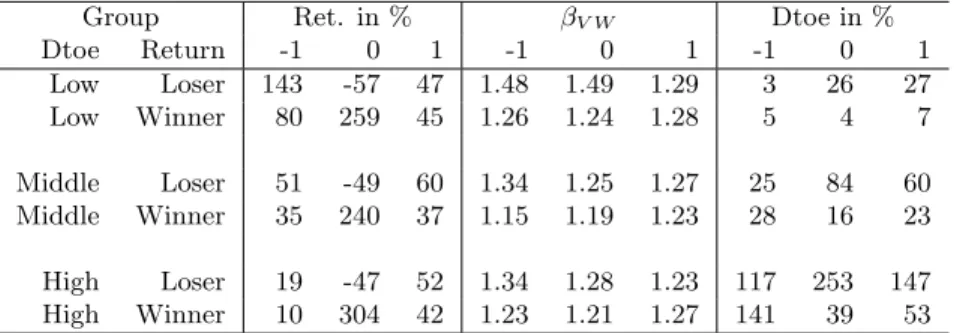
To study changes in systematic risk among both high and low financial leverage firms, we repeat the analysis in Table 1 among Dtoe sub-samples. We first group stocks into three financial leverage (Dtoe) groups in period -1 (pre-ranking period) based on 30th and 70th percentile cutoff values. We then form period 0 (ranking period) cumulative return deciles within each leverage group. Value-weighted monthly returns are formed for ranking as well as pre- and post-ranking periods for these double-sort portfolios. We then essentially repeat the empirical analysis in the previous section. Table 2 reports the results.
Consider the first two rows in both panels of Table 2 which show the results on losers and winners formed among the low initial leverage sub-sample. Both the winner and loser portfolios are essentially composed of debt-free firms in period -1. The changes in loser and winner betas are
very similar to the general case. The loserβvw decreases from 1.48 in period -1 to 1.29 in period 1,
and βmkt decreases from 1.12 to 1.06. The increase in Dtoe from 3% to 27% allows us to conclude
again that unlevered betas have decreased. In fact, the loser βhml increases relatively over time
from -0.95 to -0.39, suggesting a proportionally higher loss in growth options. On the other hand, there is essentially no change in winnerβvw, andβmktdrops slightly from 1.04 to 0.96. The winner
Dtoe undergoes a small increase from 5% to 7%, different from the large decrease seen in the Table 1. Given the changes in betas and financial leverage, unlevered betas may have slightly decreased, if at all. In terms of operating leverage, this is consistent with a firm in the right region of figure 1, where an increase ins, i.e., a decrease in operating leverage, causes a small change in β. It may also mean that for firms with an already high weight in growth options, positive news are unlikely to be related to a further increase in this weight. Namely, the condition (3) may not be met. The looserβhml of -0.95 and the winner βhml of -0.62 in period -1 suggest that these low leverage firms
have high initial growth options.
We now turn to losers and winners in the high initial leverage group, with Dtoe of 117% and 141%, respectively. For the winners, bothβvw andβmktessentially remain constant over time.
Given the large reduction in Dtoe, from 141% to 53%, the winners’ unlevered betas must have increased. The same conclusion follows from the relative decrease in βhml over time from 0.17 to
-0.08. Their terminalβhml of -0.08 corresponds to a period 1 value between groups 7 or 8, well into
the middle of the distribution in growth opportunity. These may be firms with very good news on the weight in growth options, condition (3). It is not surprising then that, as average winners, they exhibit a positive relationship between returns and unlevered betas.
We can see that even the losers with high initial financial leverage exhibit a positive operating leverage effect. Theirβvwdecreases from 1.34 to 1.23, andβmktdecreases from 1.22 to 1.17. On the
other hand, their financial leverage increases from 117% in period -1 to 147% in period 1. With an increasing financial leverage, the decrease in leveredβ implies a decrease in unlevered beta, hence a decrease in growth options. The large increase inβhml from 0.07 to 0.43 confirms this. In summary,
even firms with initially few growth options, which then suffer a further reduction of their value, still exhibit a positive operating leverage effect. This would put them on the central region of the
top plot of Figure 1, although one could have assumed that, initially already in the left region and moving further left, they would have displayed a negative relation between beta and returns.
The two middle rows of both panels in Table 2 report on the average leverage group. Again, the increase in leverage, from 25% to 60% for the losers, joint with the decrease in βvw from
1.34 to 1.24 suggest that, as the general population of losers, their unlevered betas decrease. This conclusion is also supported by the large increase inβhmlfrom -0.42 to 0.18. The winners experience
a slight decrease in leverage from 28% to 23%. The patterns of change in βvw,βmkt and βhml all
suggest that their unlevered betas increase.
4.2 Betas and growth options
The results so far are consistent with the hypotheses that growth options have higher betas and are more volatile than assets in place. We now concentrate on the first hypothesis. While the previous analysis was akin to a time series study of changes in growth opportunities, we now document the cross-sectional link between betas and firm characteristics argued in section 3 to proxy for growth options. This will also help gauge the quality of these variables as proxies of growth options.
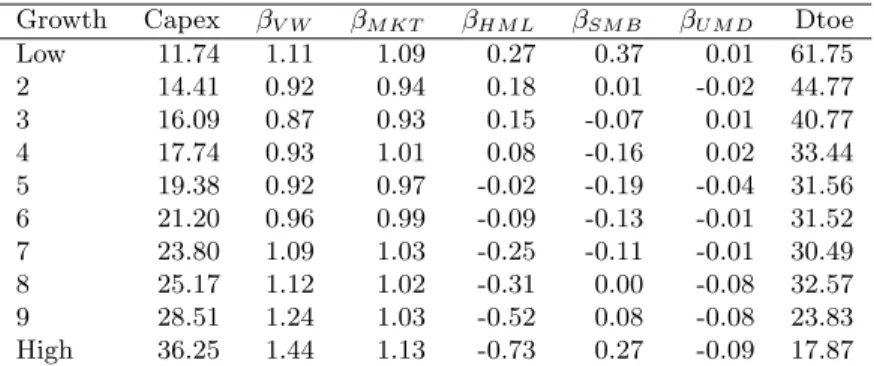
At the end of every June from 1968 to 2004, firms are allocated to increasing growth oppor-tunity groups on the basis of increasing ratios of capital expenditures to fixed assets (Capex) and market to book value of assets (Mba), and decreasing dividend yield (Div) and ratios of earnings to price (Ep) and debt to equity (Dtoe). Firms are allocated to 10 groups based on Capex and Mba, and 11 groups based on Div, Ep and Dtoe. Firms with zero dividends and debt, and non-positive earnings are grouped into portfolio 11. Table 3 reports aggregate growth opportunity proxy values, betas with respect to the value weighted NYSE, AMEX and NASDAQ market index (βvw) and
the four-factor model risk estimates (βmkt, βhml, βsmb and βumd), and aggregate debt to equity
ratios (Dtoe in %) across low-to-high growth opportunity portfolios. The numbers reported are time-series averages of portfolio values over thirty-seven overlapping 3-year post-ranking periods from July 1968-June 1971 to July 2004-June 2007.
Panel A reports results on Capex based growth deciles. The grouping highlights the cross-sectional variability in Capex, 11.74% to 36.25%, from decile 1 to 10. Remember that individual firms are allocated to portfolios based on ranking period values, and the numbers reported in Table 3 are post-ranking values. The monotonic increase of Capex from decile 1 to 10 highlights the fact that growth proxies tend to be persistent over time. Deciles 1 and 10 have leveredβvw’s of 1.11 and
1.44. Given their Dtoe’s of 61.75% and 17.87%, this means that the unlevered beta of low Capex stocks is even lower than that of high Capex stocks. Similar conclusions follow fromβmkt. Although
the relation is U-shaped, higher growth deciles tend to have larger beta’s than lower growth ones. The book-to-market risk factor βhml, argued to be inversely related to growth options, is indeed
here inversely related to Capex. The size factorβsmbhas a U-shaped relationship with Capex. This
is consistent with the fact that both low and high growth opportunity groups may include small firms. There is no discernible relationship between Capex ranking and momentum risk factor beta,
βumd.
Panel B, which reports results based on Mba sorts, leads to similar conclusions. However, the conclusions that follow from eitherβvworβmktare not as strong as those in panel A. Naturally,
there is a monotonic negative relationship between Mba and βhml. The size factorβsmb and Dtoe
are also negatively related to Mba, suggesting that low Mba groups tend to contain smaller stocks than high Mba ones.
Panels C and D report results on dividend yield (Div) and earning to price ratio (Ep) based sorts. Both of these panels lead to similar conclusions as the previous two albeit with differences due to the nature of their high growth decile 11. Decile 11 contains firms with zero dividends and non positive earnings in the ranking period. Deciles 10 (rows marked with High) in either panel tend to have higher βvw and βmkt, and lower Dtoe than deciles 1. These relationships are nearly
monotonic across deciles 1 through 10. Both proxies display an unambiguous positive relationship between proxy and beta and an inverse relationship between proxy and financial leverage. There-fore, unlevered betas must also have a positive relationship with the growth opportunity proxies. The conclusion is robust to any reasonable relationship between levered and unlevered betas, only requiring levered beta to increase with financial leverage for a given unlevered beta. We can even
infer that the positive relationship relationship between growth options and unlevered betas is stronger than that reported with equity betas. The book-to-market risk factor βhml is inversely
related to both proxies, supporting the view that unlevered betas have a positive relationship with the growth opportunity proxies.
Zero-dividend firms (row labeled Div=0) in panel C have the highest equity betas but not the lowest Dtoe. Their Dtoe of 40.26% places them somewhere between deciles 3 and 4, whereas their βhml of -0.52 places them between deciles 9 and 10. While many zero-dividend firms are
indeed growth firms, a number may just be distressed firms. The same observation can be made for non-negative earnings firms in panel D (row labeledEp≤0). While lower Ep ratios can be argued to be related to higher growth options, it is hard to extend the reasoning to negative earnings. Indeed bothβhml of 0.11 and Dtoe 74.20% indicate that these firms may have few growth options.
Theirβhml places them somewhere between deciles 4 and 5, and Dtoe places them between deciles
1 and 2.
Even though we do not consider Dtoe as a growth proxy per se, we nevertheless include it in Table 3. Panel E repeats the same analysis of this section on Dtoe sorted portfolios. The results suggest that high Dtoe firms tend to have high betas. Especially, the near monotonic decrease in
βmkt from high to low Dtoe show that the implications of the financial leverage hypothesis hold
when growth options have been accounted for by the HML factor. Not surprisingly, high Dtoe firms tend be small and low Dtoe firms tend to be large as suggested byβsmb. Once again, the zero debt
firms (decile 11) prove to be different than the rest. Theirβsmb of 0.29 places them between decile
1 and 2, suggesting that zero-debt firms are actually very small and quite different thanlow debt
firms.
The relations observed in Table 3 between growth proxies and, indirectly, unlevered betas are consistent with the hypothesis that higher growth options result in higher betas. Or, considering this hypothesis pretty uncontroversial, the results demonstrate the quality of these observables as proxies for growth options. As the firms are grouped in the ranking-period and systematic risk is measured in the post-ranking period in our analysis, the cross-sectional relationship between betas
and proxies may have some predictive power on betas. We return to this later.
4.3 Cross-sectional variation in systematic risk
The above analysis examines the relationship between betas and proxies one at a time. We now examine the joint ability of the growth opportunity proxies to explain cross-sectional variations in asset betas. To do this, we estimate the following regression:
βi,t+1 = δtXi,t + γt∆Xi,t+i,t+1 i= 1. . .50, (5)
whereXis the vector of proxies (Mba, Capex, Div, Ep, Dtoe) measured attand ∆Xis the change in X from t tot+ 1. The rational for including proxy differences is to check if, on average, recent changes in proxies have marginal explanatory power over thelong-run values of the proxies.
We form 50 portfolios to reduce measurement errors in beta estimates. In each of the thirty-seven overlapping 3-year periods covering July 1965-June 1968 to July 2001-June 2004, firms are allocated to 50 portfolios on the basis of cumulative returns. Aggregate portfolio growth proxies for this ranking period and the following 3-year post-ranking period (July 1968-June 1971 to July 2004-June 2007) are calculated at the end of each 3-year period. Portfolio systematic risk factor loadings are estimated using thirty-six monthly value weighted portfolio returns over the post-ranking period. In the above regression, the dependent variables are estimates of post-post-ranking period systematic risk and the independent variables are lagged (ranking period, denoted by t) proxies and changes (∆) in the level of proxies from ranking to post-ranking period.
We run (5) as thirty-seven overlapping cross-sectional regressions. To facilitate an economic interpretation of δ and γ, we standardize the proxies by their cross-sectional mean and variance, recomputed periodically. That is, δ is the change in β for a one cross-sectional standard deviation change in the proxy. This standardization may also be preferable if proxies exhibit strong time trends or changes through the sample period.
refer to the estimates of δ in (5). The column “mean” shows the average of the 37 estimates. Q1 and Q3 are the first and third quartiles of the distribution of the 37 estimates. “#” shows the number of estimates with the expected sign. Next to it is the the Newey-West corrected t-statistics accounting for three lags of autocorrelation. ¯R2 and ¯R2−1 report on the adjusted R-squares of the regressions, with all the independent variables and that with only the lagged (−1) variables.
The first clear result, by inspection of the R-squares is that the fit is very high. The proxies explain a large fraction of the cross-section of systematic risk. Inspection of the R-squares produces two clear results. For βvw, the R-square averages 59%, with three quarters above 52%. For βmkt,
the average R-square is lower. Second, the lagged values of the proxies, not their recent changes are at the source of this explanatory power. This is seen clearly by comparing the R-squares of the full regression in (5) with ¯R2−1 reported below (the R-square of a regression without ∆X). The coefficient estimates for the change variables ∆X confirm this result. They are mostly insignificant, and about half the time of the correct sign, as expected under the null hypothesis. The only possible exception is ∆Div, with the expected sign most of the time and a significant t-statistic. The validity of each proxy individually can also be verified. We expect positive coefficients for Capex and Mba, negative for Div and Ep. Capital expenditures and dividends are significant and with the correct sign about every single period. The coefficient of Dtoe−1 is significant and with the correct sign two-thirds of the time. This shows that one can recover the sign expected by the financial leverage hypothesis, once growth proxies have been accounted for. We note only two exceptions. Both for βvw and βvw, the slope estimate for Mba−1 is contradictory to what we would expect. The coefficient of Ep−1 forβvw has a similar pattern.
As our 50 portfolios contain fewer stocks than the standard 20 or 40 portfolios used in a typical empirical study, the measurement errors in their betas are consequently larger. However, measurement errors on a left-hand side variable do not induce a bias, they only lower the fit of (5). One goal of the regression in (5) is to precisely assess to what extent we can filter out estimation error through the use of growth opportunity proxies. In order to see the impact of having more or less than 50 portfolios in the cross-section, we re-run the regression in (5) with 25 and 100 portfolios. Panel B summarizes average fit statistics for the dependent variables in panel A as
well as book-to-market (βhml), size (βsmb) and momentum (βumd) factor loadings for 25, 50 and
100 portfolio cross-sections. As expected, having fewer portfolios in the cross-section, and thereby including more stocks in each portfolio, dramatically increases the fit.
To summarize, the lagged growth opportunity proxies explain up to two thirds of cross-sectional differences in systematic risk. The relationship between betas and each proxy most often has the desired sign given that growth options have higher betas. Recent changes in the proxies do not have marginal explanatory power over and above the lagged values of the proxies, which is consistent with a slow variation of true betas.
4.4 Return predictability and changes in growth options
Table 1 showed that loser betas decline and winner betas increase. These patterns, which arise because of losses (or gains) in growth options, could induce predictability in extreme portfolio returns if investors are slow to account for the implication of growth options on betas. Consider the following three-period scenario for a loser stock. In period one, the stock incurs negative returns. If investors anchor their beliefs on large negative stock return and the financial leverage effect but ignore potential losses in growth options, they might believe that the equity beta is higher than it really is. Assume that the market excess return is positive in period 2. If investors have not yet accounted for the loser’s decreased growth options, the loser stock rises according to the “older”
beta that is too high. In period 3, investors adjust to the new, lower beta, correcting for the excessive rise of period 2. If this is the case, we expect to see a negative relationship between the excess return in period 3 and the market return in period 2. For winners, a similar reasoning could produce a positive relationship between the winner and the lagged market returns.
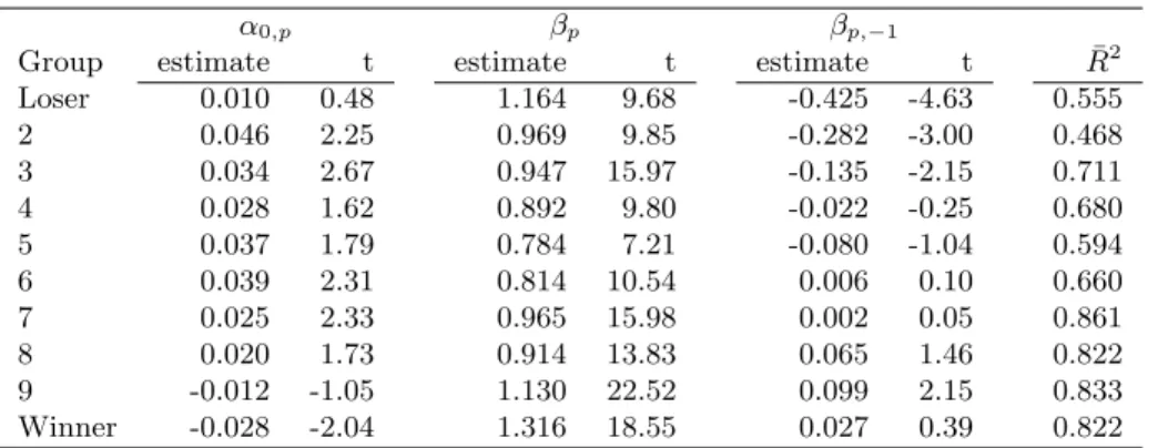
To examine this, we analyze the relationship between extreme portfolio excess returns and the previous year market excess returns. At the end of June of year t, firms are allocated to decile portfolios on the basis of past 3-year cumulative returns. Value weighted returns are tracked for 12 months over the second year after portfolio formation, resulting in a series of monthly portfolio returns covering July t+1 to June t+2. This process is repeated every year from 1968 to 2005,
providing a series of 456 monthly returns from July 1969 to June 2007. Using this second-year monthly return series, annual rolling portfolio excess returns are calculated and related to the contemporaneous and lagged market excess returns:
rp,t=α0,p+βprm,t+βp,−1rm,t−1+p,t,
Table 5 shows the results of this regression using 445 overlapping annual observations. The estimate of βp,−1 increases monotonically from losers to winners, with the exception of the one on the highest past-performing portfolio. For the losers, the estimate of βp,−1 is -0.425 with a t-statistic of -4.63. For the winners, the estimate has the correct sign but is insignificant. However, the estimate ofβp,−1for decile 9 (the second highest past-performing portfolio) is a highly significant 0.099. These results show that there is some evidence consistent with a scenario in which it takes more than a year for the market to fully incorporate changes in betas for both the losers and the winners.
5
Conclusions
The empirical literatures still makes much more case of the financial than the operating leverage effect. This is somewhat surprising given that the predictions of the financial leverage effect are somewhat at odds with the evidence. In particular, as we emphasize in this paper, betas of stocks that have experienced very high returns do not decline as the financial leverage suggests, and betas of stocks that have experienced negative returns decline significantly, which is again inconsistent with the theory.7 Moreover, the equity betas of financially distressed firms seem to decline as their financial condition deteriorates even though the unsystematic risk and total risk increase.8 While this evidence is inconsistent with the Hamada and Rubinstein leverage
7Contradictions with the predictions of financial leverage are also reported in the empirical corporate finance
literature. Firms that take actions that increase financial leverage do not experience increases in their market betas. See for example Healy and Palepu (1990), Bartov (1991), and Dann, Masulis, and Mayers (1991), Denis and Kadlec (1994), or Kaplan and Stein (1990).
8See, for example, Aharony, Jones, and Swary (1980) and Altman and Brenner (1981). They attribute the decline
adjustments, it is consistent with the hypothesis that firms increase (decrease) leverage when the value of their growth options decline (increase).
Several recent papers have linked growth opportunities to systematic risk. For instance, Berk, Green and Naik (1999), Anderson and Garcia-Feijoo (2002) and Carlson, Fisher and Giammarino (2003) show that the exercise of growth options change a firm’s systematic risk. Cao, Simin and Zhao (2007) argue that a significant portion of the upward trend in idiosyncratic risk can be explained by changes in the level and variance of growth options, as well as the capital structure of firms - subsiding the profitability based explanations in the literature. Recent general equilibrium models link the evolution of betas to latent state variables that include measures of growth options. These structural models of betas are however difficult to implement. Our cross-sectional regressions can be justified as a practical and simple reduced form for these models.
Using Myers’ (1977) description of the firm as a combination of assets in place and growth opportunities, we are able to analyze the effects of changes both in the financial leverage and the asset structure of firms on market betas. Our results suggest that the inconsistency between the financial leverage change and the change in systematic risk can at least partially be explained by the relation between past stock returns and changes in a firm’s mix between growth options, which generally have high betas, and assets in place, which generally have low betas. A dramatic decline in stock prices causes a proportionally larger reduction in the value of growth opportunities relative to the value of assets in place. Even though financial leverage increases, the reduction in the asset beta dominates and the systematic risk of losers decline. Similarly, there is an increase in the systematic risk of winner firms, in contrast to the predictions of the financial leverage effect.
We explore whether evidence of the financial leverage effect will be stronger for the stocks of highly levered firms that subsequently experience very negative returns. The high leverage of these firms should increase the importance of the leverage effect, and since these firms tend to have very few growth options, the offsetting effect should be minimized. However, we find that even for these firms, the betas of past losers tend to decrease.
which would imply that past winners and losers would either over or underreact to market moves. We present preliminary results that suggest that the losers tend to have betas that are too high, implying that they overreact to market returns. This finding will be the subject of future research.
APPENDIX: Partial derivative ofηG= ββGS with respect to the moneyness ratio.
Consider N(d1), N(d2), rf, T as in the standard Black-Scholes notation. Denote S the
un-derlying value,C the strike price, andm=S/C the moneyness ratio. The elasticity of the option
Gwith respect to the underlying S is
ηG= SN(d1) G = SN(d1) SN(d1)−Ce−rfTN(d2) = 1− 1 me −rfTN(d2) N(d1) −1 ≥1.
The partial derivative ofηG with respect to the moneyness ratiom is
∂ηG ∂m = e −rfT η2 S ∂ N(d2) mN(d1) ∂m = e−rfT η2 S − N(d2) m2N(d 1) + 1 mN2(d 1) (N(d1)Z(d2) ∂d2 ∂m −N(d2)Z(d1) ∂d1 ∂m) (6)
where Z(·) is the standard normal density function, d1 =
ln(m)+(rf+0.5σ2)T σ√T , and d2=d1−σ √ T. Note that ∂d1 ∂m = ∂d2 ∂m = 1
mσ√T, recall thatηG=SN(d1)/G, and replacemwith S C. Equation (6) simplifies as ∂ηG ∂m =− C2e−rfT S2σ√T N(d2)N(d1) σ √ T − Z(d2) N(d2) + Z(d1) N(d1) .
Galai and Masulis (1976, p. 76-77) show thatσ√T > Z(d2)
N(d2) −
Z(d1)
N(d1). Hence,
∂ηG
References
Adam, T. and Goyal, V.K., 2007, The Investment Opportunity Set and its Proxy Variables: Theory and Evidence,Working Paper, SSRN: http://ssrn.com/abstract=298048 .
Aharony, J., Jones, C.P. and Swary, I., 1980, An Analysis of Risk and Return Characteristics of Corporate Bankruptcy Using Capital Market Data, Journal of Finance, 1001-1016.
Altman, E. and Brenner, M., 1981, Information Effects and Stock Market Response to Signs of Firm Deterioration,Journal of Financial and Quantitative Analysis, 35-51.
Ball, R. and Kothari, S.P., 1989, Nonstationary Expected Returns: Implications for Tests of Market Efficiency and Serial Correlation in Returns, Journal of Financial Economics25, 51-74.
Bartov, E., 1991, Open-Market Stock Repurchases as Signals for Earnings and Risk Changes,
Journal of Accounting and Economics14, 275-294.
Beaver, W., Kettler, P. and Scholes, M. 1970, The Association Between Market Determined and Accounting Determined Risk Measures ,Accounting Review45, 654-682.
Berk, J.B., C.G. Green and V. Naik, 1999, Optimal Investment, Growth Options, and Security Returns, Journal of Finance54, 1553-1607.
Braun, P.A., D.B. Nelson and A.M. Sunier, 1995, Good news, Bad news, Volatility and Betas,
Journal of Finance 50, 1575-1603.
Campbell, J. and J. Mei, 1993, Where Do Betas Come From? Asset Price Dynamics and the Sources of Systematic Risk, Review of Financial Studies 6, 567-592.
Cao, C., Simin T., and J. Zhao, 2008, Can Growth options explain the trend in firm specific risk? Review of Financial Studies 21: 2599 - 2633.
Chan, K.C., 1988, On the Contrarian Investment Strategy, Journal of Business61, 147-163. Chopra, N., Lakonishok, J. and Ritter, J.R., 1992, Measuring Abnormal Performance, Journal of Financial Economics31, 235-268.
Dann, L.Y., Masulis, R.W. and Mayers, D., 1991, Repurchase Tender Offers and Earnings Information, Journal of Accounting and Economics14, 217-251.
DeBondt, W.F.M. and Thaler, R., 1985, Does the Stock Market Overreact?, Journal of Finance
40, 793-805.
DeBondt, W.F.M. and Thaler, R., 1987, Further evidence on investor overreaction and stock market seasonality, Journal of Finance42, 557-581.
Denis, D.J. and Kadlec, G.B., 1994, Corporate Events, Trading Activity, and the Estimation of Systematic Risk: Evidence From Equity Offerings and Share Repurchases,Journal of Finance 49, 1787-1811.
Erickson, T. and Whited, T, 2006, On the Accuracy of Different Measures of Q, Financial Man-agement, 35.
Fama, Eugene F. and French, Kenneth R., 1992, The Cross-Section of Expected Stock Returns,
Journal of Finance, 47, 427-465.
Fama, Eugene F. and French, Kenneth R., 2001, Disappearing Dividends: Changing Firm Char-acteristics or lower propenstiy to pay?, Journal of Financial Economics, 60, 3-43.
Journal of Financial Economics 3, 53-81.
Goyal, V.K., Lehn, K. and Racic, S., 2002, Growth Opportunities and Corporate Debt Policy: The Case of the U.S. Defense Industry, Journal of Financial Economics64, 35-59.
Hamada, R.S., 1972, The Effects of the Firm’s Capital Structure on the Systematic Risk of Common Stocks,Journal of Finance 27, 435-452.
Healy, P.M. and Palepu, K. G., 1990, Earnings and Risk Changes Surrounding Primary Stock Offers,Journal of Accounting Research 28, 25-48.
Jagannathan, R. and Z. Wang, 1996, The Conditional CAPM and the Cross-Section of Expected Returns, Journal of Finance51 (1), 3-53.
Jones, S.L., 1993, Another look at time-varying risk and return in a long-horizon contrarian strategy,Journal of Financial Economics 33, 119-144.
Kaplan, S.N. and Stein, J.C., 1990, How risky is the debt in highly leveraged transactions?,
Journal of Financial Economics 27, 215-245.
Kester, W.C., 1984, Today’s Options for Tomorrow’s Growth,Harvard Business Review, March-April, 153-160.
Kester, W.C., 1986, An Options Approach to Corporate Finance, in Edward I. Altman, ed.:
Handbook of Corporate Finance(New York: Wiley), 5.1-5.35.
Myers, S., 1977, Determinants of Corporate Borrowing,Journal of Financial Economics5, 147-175. Pindyck, R., 1988, Irreversible Investment, Capacity Choice, and the Value of the Firm,American Economic Review 78, 969-985.
Rosenberg, B. and McKibben, W., 1973, The Prediction of Systematic and Specific Risk in Common Stocks,Journal of Financial and Quantitative Analysis, 317-333.
Rosenberg, B., 1974, Extra-Market Components of Covariance in Security Returns, Journal of Financial and Quantitative Analysis, 263-274.
Rosenberg, B., 1985, Prediction of Common Stock Betas,Journal of Portfolio ManagementWinter, 5-14.
Rubinstein, M.E., 1973, A mean-Variance Synthesis of Corporate Financial Theory, Journal of Finance28, 167-181.
Smith, W.S., Watts, R.L., 1992, The Investment Opportunity Set and Corporate Financing, Dividend and Compensation Policies,Journal of Financial Economics 32, 263-292.
Skinner, D.J., 1993, The Investment Opportunity Set and Accounting Procedure Choice, Journal of Accounting and Economics 16, 407-445.
Table 1: Portfolio characteristics based on cumulative returns in the ranking period Firms are allocated to deciles ranked by cumulative returns over thirty-four overlapping 3-year periods covering July 1968-June 1971 to July 2001-June 2004. The column headers 0, -1, and 1, refer to the ranking period, and the two 3-year periods preceding (July 1965-June 1968 to July 1998-June 2001) and following (July 1971-June 1974 to July 2004-June 2007) the ranking period. Value-weighted monthly portfolio returns are formed for ranking as well as pre- and post-ranking periods. Panel A reports cumulative returns (Ret. in %), betas with respect to the value weighted
NYSE, AMEX and NASDAQ market index (βvw) and aggregate debt to equity ratios (Dtoe in %)
for decile portfolios. Panel B shows the four-factor model risk factor loadings (βmkt,βhml,βsmb and
βumd). The numbers reported are time-series averages of portfolio values. Panel A: Returns, CAPM betas and leverage
Group Ret. in % βV W Dtoe in %
Return -1 0 1 -1 0 1 -1 0 1 Loser 75 -53 48 1.35 1.34 1.26 25 82 58 2 58 -28 48 1.21 1.17 1.12 28 60 45 3 53 -10 52 1.07 1.07 1.01 27 51 43 4 40 7 47 1.03 0.98 0.95 36 48 45 5 41 23 48 0.99 0.91 0.93 38 47 43 6 47 40 47 0.96 0.95 0.95 37 37 36 7 39 61 45 0.96 0.93 0.95 36 32 34 8 38 89 45 0.98 0.96 0.99 43 29 30 9 41 134 49 1.04 1.04 1.07 42 24 28 Winner 40 264 40 1.21 1.20 1.27 46 16 23
Panel B: 4-factor model parameter estimates
Group βM KT βHM L βSM B βU M D Return -1 0 1 -1 0 1 -1 0 1 -1 0 1 Loser 1.12 1.17 1.13 -0.61 -0.26 -0.07 0.25 0.39 0.56 -0.02 -0.51 -0.22 2 1.06 1.10 1.11 -0.34 -0.15 0.04 0.10 0.22 0.30 -0.01 -0.29 -0.05 3 1.01 1.06 1.05 -0.18 -0.05 0.06 0.06 0.11 0.09 -0.02 -0.25 -0.12 4 1.02 0.99 1.00 -0.12 0.01 0.17 -0.05 0.03 0.01 -0.03 -0.25 -0.11 5 0.99 0.94 0.99 -0.06 0.07 0.17 -0.06 -0.02 -0.04 -0.05 -0.15 -0.09 6 1.00 0.96 0.98 -0.01 0.02 0.07 -0.03 -0.12 -0.11 -0.04 -0.04 -0.03 7 0.99 0.94 0.96 -0.01 0.04 -0.01 -0.07 -0.05 -0.12 -0.02 0.03 -0.03 8 0.98 0.99 0.97 -0.04 0.07 -0.11 -0.02 -0.09 -0.10 -0.06 0.09 0.00 9 1.02 1.01 0.97 -0.10 -0.07 -0.29 0.10 -0.01 -0.07 -0.06 0.15 0.03 Winner 1.07 1.02 1.04 -0.23 -0.42 -0.58 0.30 0.20 0.07 -0.02 0.30 0.04
Table 2: Portfolio characteristics based on a double sort: Financial leverage sorts in the pre-ranking period and cumulative return sorts in the ranking period
Firms are first allocated into three financial leverage (Dtoe) groups in the pre-ranking period -1 based on 30th and 70th percentile cutoff values. Then, within each leverage group, firms are grouped into cumulative return deciles in the ranking period 0. Please see Table 1 for the definition of ranking, and pre- and post-ranking periods. Panel A reports cumulative returns (Ret. in %), betas with
respect to the value weighted NYSE, AMEX and NASDAQ market index (βvw) and aggregate debt
to equity ratios (Dtoe in %) for double sort portfolios. Panel B shows the four-factor model risk
factor loadings (βmkt, βhml, βsmb and βumd). The numbers reported are time-series averages of
portfolio values.
Panel A: Returns, CAPM betas and leverage
Group Ret. in % βV W Dtoe in %
Dtoe Return -1 0 1 -1 0 1 -1 0 1 Low Loser 143 -57 47 1.48 1.49 1.29 3 26 27 Low Winner 80 259 45 1.26 1.24 1.28 5 4 7 Middle Loser 51 -49 60 1.34 1.25 1.27 25 84 60 Middle Winner 35 240 37 1.15 1.19 1.23 28 16 23 High Loser 19 -47 52 1.34 1.28 1.23 117 253 147 High Winner 10 304 42 1.23 1.21 1.27 141 39 53
Panel B: 4-factor model parameter estimates
Group βM KT βHM L βSM B βU M D Dtoe Return -1 0 1 -1 0 1 -1 0 1 -1 0 1 Low Loser 1.12 1.22 1.06 -0.95 -0.59 -0.39 0.38 0.30 0.55 0.05 -0.55 -0.21 Low Winner 1.04 0.98 0.96 -0.62 -0.71 -0.88 0.24 0.13 -0.01 0.02 0.27 -0.02 Middle Loser 1.15 1.15 1.21 -0.42 -0.05 0.18 0.25 0.44 0.59 -0.05 -0.48 -0.12 Middle Winner 1.06 1.06 1.07 -0.16 -0.25 -0.48 0.31 0.15 0.07 -0.07 0.29 0.07 High Loser 1.22 1.22 1.17 0.07 0.44 0.43 0.55 0.86 0.85 -0.19 -0.41 -0.21 High Winner 1.13 1.10 1.14 0.17 0.10 -0.08 0.69 0.51 0.40 -0.12 0.22 0.09
Table 3: Systematic risk characteristics versus growth proxies
At the end of every June from 1968 to 2004, firms are allocated to increasing growth opportunity groups on the basis of increasing ratios of capital expenditures to fixed assets (Capex) and market to book value of assets (Mba), and decreasing dividend yield (Div) and ratios of earnings to price (Ep) and debt to equity (Dtoe). Firms are allocated to 10 groups based on Capex and Mba, and 11 groups based on Div, Ep and Dtoe. Firms with zero dividends and debt, and non-positive earnings are grouped into portfolio 11. This table reports aggregate growth opportunity proxy values, betas
with respect to the value weighted NYSE, AMEX and NASDAQ market index (βV W) and the
four-factor model risk four-factors (βM KT, βHM L, βSM B and βU M D), and aggregate debt to equity ratios
(Dtoe in %) across low-to-high growth opportunity portfolios over thirty-seven overlapping 3-year post-ranking periods from July 1968-June 1971 to July 2004-June 2007. Growth opportunity proxies and debt to equity ratios are measured at the end of a given 3-year period. The numbers reported are time-series averages of portfolio values.
Panel A: Growth proxy is increasing in percent Capex
Growth Capex βV W βM KT βHM L βSM B βU M D Dtoe
Low 11.74 1.11 1.09 0.27 0.37 0.01 61.75 2 14.41 0.92 0.94 0.18 0.01 -0.02 44.77 3 16.09 0.87 0.93 0.15 -0.07 0.01 40.77 4 17.74 0.93 1.01 0.08 -0.16 0.02 33.44 5 19.38 0.92 0.97 -0.02 -0.19 -0.04 31.56 6 21.20 0.96 0.99 -0.09 -0.13 -0.01 31.52 7 23.80 1.09 1.03 -0.25 -0.11 -0.01 30.49 8 25.17 1.12 1.02 -0.31 0.00 -0.08 32.57 9 28.51 1.24 1.03 -0.52 0.08 -0.08 23.83 High 36.25 1.44 1.13 -0.73 0.27 -0.09 17.87
Panel B: Growth proxy is increasing in percent Mba
Growth Mba βV W βM KT βHM L βSM B βU M D Dtoe
Low 91.77 1.05 1.08 0.53 0.41 -0.05 71.94 2 101.57 1.06 1.11 0.52 0.24 -0.10 87.20 3 105.86 0.99 1.09 0.51 0.08 -0.09 88.80 4 118.80 1.00 1.06 0.34 0.04 -0.02 58.63 5 129.92 0.95 1.02 0.21 -0.02 0.00 48.22 6 141.10 1.00 1.03 0.08 -0.08 -0.01 39.24 7 157.88 1.02 1.01 -0.01 -0.05 0.00 33.38 8 181.95 1.02 0.99 -0.15 -0.06 -0.04 22.16 9 233.19 1.01 0.95 -0.36 -0.09 -0.02 13.47 High 364.59 1.09 0.93 -0.70 -0.11 -0.02 5.98