Use of Numerical Models as Data Proxies for Approximate Ad-Hoc Query Processing

(1)

A

pproved for public release; further dissemination unlimited

Lawrence

Livermore

National

Laboratory

U.S. Department of Energy

Preprint

UCRL-JC-??????

Use of Numerical Models as Data

Proxies for Approximate Ad-Hoc

Query Processing

R. Kamimura, G. Abdulla, C. Baldwin, T. Critchlow,

B. Lee, I. Lozares, R. Musick, and N. Tang

This article appears in the Proceedings of the 7

th

Joint Conference

on Information Systems, Research Triangle Park, NC, September

2003.

(2)

DISCLAIMER

This document was prepared as an account of work sponsored by an agency of the United States

Government. Neither the United States Government nor the University of California nor any of their

employees, makes any warranty, express or implied, or assumes any legal liability or responsibility for

the accuracy, completeness, or usefulness of any information, apparatus, product, or process disclosed, or

represents that its use would not infringe privately owned rights. Reference herein to any specific

commercial product, process, or service by trade name, trademark, manufacturer, or otherwise, does not

necessarily constitute or imply its endorsement, recommendation, or favoring by the United States

Government or the University of California. The views and opinions of authors expressed herein do not

necessarily state or reflect those of the United States Government or the University of California, and

shall not be used for advertising or product endorsement purposes.

This is a preprint of a paper intended for publication in a journal or proceedings. Since changes may be

made before publication, this preprint is made available with the understanding that it will not be cited

or reproduced without the permission of the author.

This report has been reproduced directly from the best available copy.

Available electronically at http://www.doc.gov/bridge

Available for a processing fee to U.S. Department of Energy

And its contractors in paper from

U.S. Department of Energy

Office of Scientific and Technical Information

P.O. Box 62

Oak Ridge, TN 37831-0062

Telephone: (865) 576-8401

Facsimile: (865) 576-5728

Available for the sale to the public from

U.S. Department of Commerce

National Technical Information Service

5285 Port Royal Road

Springfield, VA 22161

Telephone: (800) 553-6847

Facsimile: (703) 605-6900

Online ordering: http://www.ntis.gov/ordering.htm

OR

Lawrence Livermore National Laboratory

Technical Information Department’s Digital Library

(3)

1

Use of Numerical Models as Data Proxies for

Approximate Ad-Hoc Query Processing

R. Kamimura

1

, G. Abdulla

1

, C. Baldwin

1

, T. Critchlow

1

, B. Lee

2

, I. Lozares

1

, R. Musick

3

,

N. Tang

1

CASC, Lawrence Livermore National Laboratory, CA

2

Department of Computer Science, University of Vermont, VT

3

Ikuni, Inc., CA

Abstract

As datasets grow beyond the gigabyte scale, there is an increasing demand to develop techniques for dealing/interacting with them. To this end, the DataFoundry team at the Lawrence Livermore National Laboratory has developed a software prototype called Approximate Adhoc Query Engine for Simulation Data (AQSim). The goal of AQSim is to provide a framework that allows scientists to interactively perform adhoc queries over terabyte scale datasets using numerical models as proxies for the original data. The advantages of this system are several. The first is that by storing only the model parameters, each dataset occupies a smaller footprint compared to the original, increasing the shelf life of such datasets before they are sent to archival storage. Second, the models are geared towards approximate querying as they are built at different resolutions, allowing the user to make the tradeoff between model accuracy and query response time. This allows the user greater opportunities for exploratory data analysis. Lastly, several different models are allowed, each focusing on a different characteristic of the data thereby enhancing the interpretability of the data compared to the original. The focus of this paper is on the modeling aspects of the AQSim framework.

1. Introduction

Advances in computer technology and decreasing hardware costs have facilitated the ease by which large volumes of data are measured, generated, and stored. While this is viewed as an information bonanza, the result has often been a flood of data with limited means of making effective use of it. The central problem is that of size. When datasets reach the gigabyte level and beyond, storing the information as well as being able to interact with it become increasingly constrained in space or time or in some cases both. While research is being conducted in developing mass storage devices, there will always be limited resources to accommodate the dataflow. A related issue is that of data compression as ideally one would like to store as minimal information as possible to maximize the effectiveness of the hardware. But even if the spatial constraints are resolved, the issue of how to interact with the data within a reasonable period of time still remains. Data analysis tasks such as asking an ad-hoc query become ineffective for large scale data sets if the time to find and retrieve the exact answer to the query posed is often longer than the user is willing to tolerate. This is especially true if the scientist is in an exploratory data analysis mode and has several questions that they would like to examine.

To deal with time constraint problem, one approach that has been used recently is approximate querying systems, which

seek not to provide an exact solution to the posed query but an approximate one. The rational is that the user may prefer a fast, approximate answer as they explore the dataset to develop a better understanding of truly interesting queries and/or regions. To this end, Acharya, et.al., 1999, Acharya, et.al., 1999a, Chakrabarti’s, et.al., 2000, Ioannidis and Poosala (1999), Vitter and Wang (1999), Vitter and Wang (1998) have developed different approaches for dealing with aggregate and range queries in an approximate fashion.

However, the emphasis in the above approaches focused on the issue of a fast query response system and did not specifically address the issue of storing such large data sets. This latter point is important if the user should wish to revisit the data set which, owing to its size, will often have to be moved to tertiary storage as is often the case with scientific simulations. Accessing the data at such locations is often prohibitive time-wise and should be avoided if possible. As a result, what is needed is a system that not only allows approximate ad hoc queries but also provides a compact representation of the data that is far easier to store and access compared to the original. A survey of the literature uncovers that Hachem, et.al. (1995) have implemented a system where polynomial regression models are used to model non-spatial data and the regression coefficients are stored in the database. In response to a query, the data are reconstructed from models. Such a system provides the benefits of approximate query response but at a far smaller storage cost.

Following a similar approach independently, the DataFoundry team at Lawrence Livermore National Laboratory has developed the Approximate Ad-hoc Query Engine for Simulation Data (AQSim). The goal of AQSim is to provide a software framework that not only allows relatively fast interactive adhoc query capability of terabyte scale data but also provides a compact representation of the data. This is achieved by constructing mathematical models of the data at different resolutions. In effect, these models act as data “proxies” and perform in their place in response to a query submission. This has several benefits. First, the different resolutions of the data allow the user to trade off time for accuracy. Second, along with an index file, only the model parameters are stored in a file. As this number is often smaller than the original dataset size, the shelf life of the dataset can be extended. The user can send the original data to archival storage but can query using the model parameters for data reconstruction. Finally, as mathematical models often characterize different facets of the data, the model parameters themselves may provide additional insights not apparent when just dealing with the original raw values. Thus, in contrast to Hachem, et.al.’s work where only one model is used to address the different query needs of the scientists, AQSim uses multiple

(4)

models. While AqSim is built for dealing with the spatio-temporal nature of the scientific simulations for the Accelerated Strategic Computing Initiative program (ASCI), the framework is generic enough to be applied to other domains that deal with terabyte scale datasets.

In this paper the focus is on the modeling aspect of the AQSim framework. Section 2 provides a brief overview of the entire system. Section 3 discusses the modeling issues that need to be addressed. Current results of AQSim are presented in Section 4. Finally, conclusions and future work are discussed in Section 5.

2. AQSim Framework

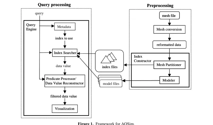
Figure 1 shows the AQSim framework under construction. The system is divided into two phases: preprocessing and query processing. The goal of the first phase is to take the original data and build the model files and index structures necessary to support the query-processing step that follows it. As the focus will be on developing a compact and accurate data proxy, more time and computational effort is placed in this initial period. The rational is to concentrate the computational burden when the data is close at hand and still away from the user. In this way, the time spent during query processing which is where the user is expected to spend the bulk of their time can be minimized. The input to the preprocessing will be the original data itself, the selection of models to be implemented, and a partitioning scheme.

To achieve the approximate query answer capability, the data is statistically characterized and modeled at different resolutions. These resolutions are created by partitioning the data into progressively smaller subunits and then subsequently modeling each of these partitions by the selected models. This procedure is repeated until the partitioning reaches a selected threshold upon which it is terminated. The current partitioning scheme is bisect the data along each of the spatio-temporal

coordinates (x,y,z,t), thereby creating a 16-way tree. The rational was to take advantage of the spatio-temporal nature of the scientific simulations that were being studied. In any event, the end result is a tree structure. The root node represents the entire data set with each of its children (and subsequent children) representing a different subset of the data. Each node contains the following statistics about the data that was in it: number of data points, number of models built on the data in that node, the types of models used, model errors, and for each variable, its corresponding mean, standard deviation, minimum and maximum values. As will be discussed later, the index searcher will use this information when searching for a response to a query.

If directly implemented as stated above, one problem that is immediately encountered is that is it unlikely that a model built with a majority of the data is accurate or that it can be built in a reasonably short time. Hence, to balance the time-accuracy tradeoff, the key is to fix the model complexity for each node. The supposition is that as the data becomes increasingly partitioned, the localization will increase the likelihood that a model of fixed complexity will be able to model the behavior reasonably well. A comparable analogy is to break a nonlinear curve into piece-wise components which depending on the length of the component can be sufficiently linear for linear regression models to be built on the components. Naturally, there is no guarantee that the accuracy will reach what is desired but this combination of partitioning and modeling is being used to a first approximation. As will be discussed in Section 5, identifying metrics as to when to build models as opposed to having them built at every node is a research topic. If such a metric is found, it can decrease storage and computational costs of building models to only those that are needed.

Once the partitioning and model building is done, the output from the preprocessing stage is an index file containing all the node information along with the corresponding model files. It

Index Constructor Mesh Partitioner index files Mesh conversion mesh file reformatted data model files

Query processing _{Preprocessing}

Modeler Index Searcher data value Query Engine Predicate Processor/ Data Value Reconstructor

Metadata

index to use query

Visualization filtered data value

Index Constructor Mesh Partitioner index files Mesh conversion mesh file mesh file reformatted data model files model files

Query processing _{Preprocessing}

Modeler Index Searcher data value Query Engine Predicate Processor/ Data Value Reconstructor

Metadata

index to use query

Visualization filtered data value

(5)

3 is important to note the original data is not stored in either the index or model files. The nodes only contain the information listed above along with pointers to its children. The model files only contain information about the model parameters that were used for each node. Hence, it is hoped that these subsequent files will be smaller in size than the original data. So, if a particular section of the data is to be reconstructed one needs to know which node and which model to use to reconstruct that particular subsection.

The query-processing phase is the side that deals primarily with the user and is the means by which they present queries to the system. After the index and model files have been initialized and read in by the system, the user can pose adhoc queries to the query engine. The query engine then identifies the variables and predicates in the query and selects an index to use based on the metadata. An index searcher then examines the index nodes using the statistical information contained within them to determine which nodes (and models) are most relevant to the query. A list of candidate nodes is then sent to a predicate processor/data value reconstructor, which then reconstructs the data and formulates a response. During this period, the user can specify the accuracy of the response and this information will be used to determine how deep within the tree to search. Once the data has been reconstructed it is then sent to a visualization tool to view the results.

3. Modeling Issues

As the models act as proxies for the data, it is essential that a set of criteria or metrics be developed to assess the feasibility of using a particular model for the AQSim system. Initially, our focus was on traditional modeling criteria such as model error and complexity as these are often used to assess model performance. Unfortunately, due to the scale of the data involved and the tight coupling with respect to queries, these criteria were found not to be particularly informative. For example, model error as a measure of model accuracy was relevant but its importance was somewhat reduced to due to the multiresolutional structure of the tree which reconstructs the data, in principle, at a higher accuracy (baring overfitting) as the leaves of the tree are approached. But as this is nevertheless an important measure, mean square error or root mean square error was selected as a model error metric to establish a standard.

Similarly, model complexity was also viewed at first as important but oftentimes metrics such as Akaike or Bayes information criteria are often used to compare among a set of models, balancing model simplicity with error, Myung (2000). The drawback was that the size of the datasets precludes the building of several models or even iterating over the same model to obtain a better fit.

As such, a new set of criteria has been developed focusing primarily on the computational and storage cost of building models as well as examining their applicability for dealing with various query types. The former has been simply termed as model building whereas model queryability is used for the latter.

3.1. Model building

Here, the goal is to assign some semi-quantitative measure to how computational expensive building a model can be as well as the associated cost of storing the model parameters. Assume that yi is the ith variable of the original data and xiis a vector of

independent variable(s) associated with yi. xi is denoted as a

vector to emphasize generic-ness. X can be another variable in the data set (univariate model), a collection of other variables (multivariate model), or simply an index. With this in mind, the model is formulated as such:

) ; ( _i _i

i f

y = x θ (1)

where f denotes the model itself and θθθθi is a vector of model

parameters (coefficients)

The computational cost of building the model (equation 1) per node is expressed in big O-notation (Cormen, et.al., 1998):

O(F(n)) + r*O(G(n)) (2) where n represents the number of samples in a given node, O(F(n)) represents the cost of building the initial model where F(n) also includes any model specific preprocessing steps, r is the number of steps needed to refine the model to either a desired level of complexity or error ( r > 0), O(G(n)) is the cost of the model refinement steps where G(n) represents the functional form of the cost as a function of the number of samples. G(n) may be the same as F(n) or functionally different. F(n), G(n) represent the generic function forms. (eg. they can be n, nlogn, n2, etc). The term “r” encapsulates the iterative nature of the refinement process dealing with issues such as increasing the number of knots in a B-spline or the processing steps for determining the appropriate wavelet coefficient threshold values to achieve a target error. If the user desires a more accurate model, the price is the additional computational time required to refine the model.

Once the model has been built, there is the issue of the storage size of the model. The storage cost per index tree node, s, can be estimated as

s = p * v + i (3)

where i is the size of index mapping, v is the number of variables, and p is the parameter size per variable, which is the size of θθθθi(number of coefficients, for example) multiplied by

the size of the data type used (e.g., integer, float, double). In general, the parameter size cannot be readily estimated since it is dependent on the data distribution and the level of error specified. However, if the model complexity is set, the size can be estimated as the user explicitly limits the number of parameters per variable. Finally, the index mapping may or may not exist depending on the model type but is presented for completeness. It represents any additional bookkeeping that may be required to reconstruct the data.

3.2. Model building trade-offs

The above presents a formalism to estimate the cost of model construction in both memory and computation. The following general observations can be made:

• As partitioning occurs, n becomes smaller so the computational cost goes down although functionally equation 2 remains the same.

• If lower modeling error is desired, this usually translates into an increase in r of equation 2 -- increasing the number of iterations to bring the model to convergence. θθθθi is also

likely to increase (but not always) in size as additional parameters are needed to bring the model to target error levels. Depending on the modeling algorithm used, the number of iterations and the parameter size may or may not be tied with each other. In the case of regression, additional model terms are introduced to reduce model error so the iteration and parameter size are linked. On the other hand, with neural networks, the weights of system do

(6)

not change in number but their values are adjusted with each iteration cycle.

To summarize, to assess the full impact of model building, the following need to be known:

• Initial model cost – O(F(n))

• Model refinement cost – O(G(n))

• Model complexity (related to error as well) – this sets r and size of θθθθi

• Bookkeeping – is it needed and if so how big

Once this is known, equations 2 and 3 can be used to estimate cost and storage requirements on a per node basis for a given model. This information then forms a basis by which different models can be compared on model construction/memory storage criteria. To consider the effect of the entire data set, multiply the above estimates (equations 2 and 3) by the number of nodes in the index tree and adjust for n in the different nodes.

3.3. Model queryability

As mentioned previously it is not sufficient that the model simply reconstruct the data to within a small error as the nature of the gigabyte+ scale data make build such models computationally expensive. Ideally the most useful models are the ones that not only reconstruct data well but are amenable to dealing with a variety of queries. It is this issue of “queryability” that will be discussed in this section.

In brief, queryability considers the question “Short of reconstructing the data, how can the model structure of functionality be used to answer the query?” All the models in AQSim have the capability of reconstructing the data to varying degrees of accuracy. However, some models will capture different aspects of the data structure in their formulation than others. For example, with the case of simple linear regression of y = mx + b the parameter m contains information on the rate of change of y with respect to x. This ease of information access is what needs to be characterized in order to effectively determine which model to use to answer a query. Ideally, the goal is to arrive at a mapping that would associate particular models to certain query types. To achieve this, a set of criteria is needed to assess the feasibility of different model types in the context of the queries that may be presented.

As AQSim will incorporate multiple models, understanding the applicability or relevance a particular model may have in the context of responding to a query is essential. A survey of the literature does not reveal any type of model/query association metrics and points to a need to develop one for this system. In addition, considering the variety and complexity of queries that may be asked, it is unlikely that a single quantitative metric can be arrived to measure queryability. Instead, it may be more feasible to break the assessment into “semi-qualitative” and “semi-quantitative” components. The former focuses on breaking down the query types into different categories such as the one listed below. (This is a rough list and not meant to be exhaustive or mutually exclusive)

1) range – for a given input, find the associated output 2) aggregate – find how many data samples satisfy a

given query predicate

3) scale-dependent patterns/ “dynamicity” – find similar types of behavior at the specified scale

4) topological – find the samples that are within a specified target range

5) variable interactions – find the data samples that satisfy the specified variable relationships

6) area/volume effects – find the area or volume for a particular variable condition

7) domain-specific – user defines a function of interest in the query predicate

Each model candidate is “graded” on their ability to deal with the different categories, specifically whether they are able to address such queries (apart from brute force data reconstruction) and how accurately. An additional consideration may be to assign a weight to the different query types as to how likely they are to occur and/or how important they are. Ideally, the models that are selected for the AQSim should be complementary with respect to each other to minimize redundant coverage. In this regard, models that are domain-specific probably should probably be always included since it is assumed that their construction contains domain-relevant information, which would not to be readily available from the original data. But again this need may have to be balanced with respect to how often would that kind of information is requested. The semi-quantitative aspect may be viewed as the number of data processing steps and/or computational time required to process the model to arrive at the desired output. For example, if the query is of a range type, specifically “Find all x for this value of y” and two models exist -- one model is that of a spline regression (y = f(x)) and the other is a wavelet (x = f(i), y = f(i)), estimating how long would it take each model to arrive at an answer is an interesting metric. The former would require solving for the roots of the polynomial whereas the wavelets may simply reconstruct all the data for given range and then apply a filtering operation to isolate the relevant answers. It should be emphasized that this type of analysis is semi-quantitative in nature since it is highly dependent on the distribution of the data and initial starting points.

3.4. Model-query interaction

This section focuses on the cost of interacting with a model to get the desired answer to the query. The knowledge gained here allows models to be compared on the basis of how computationally expensive they are when dealing with queries. Assume that the user poses the query in the form, “Given yi,

provide h(xi).” Again, yi denotes a variable of the original data

set. H(xi) is presented here as the generic output needed to

answer the query. In its simplest form, h(xi) = xi where xi is

similar to the one used in equation 1 with the focus on either a single original variable or a collection of variables (since the index is not part of the original data the user is not likely to make any inquiries about it). In a more advanced form, h(xi)

may be a user-defined function that uses as input xi. To answer

the query (find h(xi) for yi), the procedure is to start with what

the model provides and then process the results until the desired information becomes available. This cost of answering a query essentially can be estimated by equation 4 (Corman, et.al., 1998):

∑

₌ = m₌ i i m i i n O f n f O 1 1 )) ( ( )) ( ( (4)

where m = number of processing steps required, O(fi(n)) is the

computational cost associated with each processing step i, n = number of samples. It is assumed that the processing costs are linearly additive. The key lies in what is meant by a processing step. Consider that there exists a model for a single variable, x = f(i) where i is an index, and another model for a different variable, y = g(j) where j is a different index. For a “Find the x associated with y,” this would require creating or learning the

(7)

5 mapping between i and j, say i = m(j), if the appropriate x-y pairs are to be uncovered. This mapping would be a processing step in addition to the one where for the given y, the j’s would have to be generated, j = g-1(y), – another processing step. The cost of answering the queries requires both steps be processed.

As another example, assume that xiof equation 1 is some

multivariate collection and again the query is “Find the xi

associated with yi.” This can be answered by solving the

inverse of equation 1 and, for illustrative purposes, it is further assumed that this is O(n2) :

)

(

1 i

y

f

−

=

i

x

(5)

This is not the only approach to solving the problem. A naïve but simple alternative would be to reconstruct the data for all available yi and shift through to look for the xi’s of interest.

Assume for the sake of argument that this is of O(nlogn) for the generation and O(nlogn) for the shifting. Now, it is not clear as to which approach, the solver or the naïve one, is better. The solver has one processing step but it is computationally expensive. The naïve way involves two steps but individually they are not as expensive. So, depending on which route, as well as the sample size involved, the cost can vary. So, equation 4 should be evaluated on both routes to obtain an estimate of the cost with the goal of selecting the processing route that is cheaper. Given two models, it is important to determine how much it would cost to use one model over another by breaking it down to the number of processing steps required to generate the appropriate response, and the cost associated with each step for each model. The final decision based on choosing the lesser total of the two.

Note that this analysis can be expanded to go further than just finding xi but can also consider the cost of generating h(xi).

The formulation of equation 4 is such that it can be used to evaluate model performance against a range of query types. This is done by the formulation of h(xi). For range queries, it

may be sufficient to have h(xi) = xi. To examine how they fare

on topological queries, choose the appropriate h(xi) and then

estimate the costs. This analysis, however, is not complete because recall the model also has θθθθI’s. While the emphasis has

been on largely obtaining h(xi) from xi, it is possible that the

parameters themselves readily lend to h(xi) and this should be

considered when evaluating a model. For example, “dynamicity” is reflected in the wavelet coefficients, while information such as rate of change can be observed in the coefficients of linear regression models. Note that equation 4 simply focuses on the processing steps but is not concerned whether they involve parameters or xi’s. The complementary

criterion to the model building described in section 3.1 is to then select the model with the lowest cost for a desired query type or types.

In summary, for each model under consideration, it is recommended to first use equations 2, 3, and 4 to assess the computational cost and memory needs as the model is used against different query types (if applicable). Note, that these equations have some adjustable parameters, such as m and r, and these will depend on the accuracy sought and the query being asked. In general, the model that has the lowest cost in computation and memory for a given query is a strong viable candidate. This analysis has not considered tree search costs since this cannot be determined from the model structure itself but may prove to be substantial for some models (to obtain a target accuracy) compared to others. The final assessment should also consider this search cost as well once the index searching protocol has been finalized. In short, a model that

answers the query of interest with minimal total computational cost and memory is a strong candidate to be considered for AQSim.

4. Results

Below is an illustration for a simple wavelet (finite length) model and a statistical model using the mean as the model using the criteria discussed in section 3. The results have been broken into model building and model-query interaction and, for the latter, with some selected query types of interest and the memory usage.

4.1. Model building

Modeling building incurs the following computational cost. wavelet stat

2*O(n) + O(n ln n) N*O(n)

Here, the cost for the wavelets includes the cost of scanning through the data (a conservative high estimate is presented) and the need to cull the wavelet coefficients to obtain a target error. The scanning considers the cost of the downsampling when performing the wavelet decomposition. Note that, as the wavelet model is inherently multiresolutional, it can in theory just work on the parent node and achieve a high level of accuracy. As to the statistics model, the large N refers to the total number of nodes in the index tree. To achieve a desired level of accuracy, the data will be partitioned to the resolution that is desired. If the data is widely distributed or high precision is requested, N can approach or exceed n in value. The reason is that if each leaf node is believed to contain a single point then minimum N = n, but as this is only the leaves and not the rest of the tree, N>n.

4.2. Model-query interaction

The following three query cases provide an overview of the computational cost the two models incur when queried.

Range query:

wavelet stat_model O(n) + O(n) O(ln N)

reconstruct/filter find relevant input

In the case of the wavelet, the extreme case is considered where the entire data is reconstructed and then filtered upon to find the values of interest. To simplify the analysis, only filtering was considered. (It is possible to have the wavelet reconstruct selected areas of the data, but this would be covered by the bookkeeping and its function form is not clearly known for the purposes of this exercise.) It may be possible to shorten this to O(d) where d << n if a mapping can be achieved by linking the distribution of the data values to particular wavelet coefficients. For the statistics model, the cost is largely in searching a tree of N nodes to find the model values that satisfy the query.

Dynamicity query:

wavelet stat_model O( ln C) O(n) + O(G(n))

Since the wavelet models stores information about the dynamicity (variable activity) in the wavelet coefficients, this would simply be a search over these model parameters, C – number of wavelet coefficients. For the case of statistical model, it would require a reconstruction of the data followed by further processing of the data to define the dynamicity function. If something aside from standard deviation is desired, this can

(8)

be costly. For example, G(n) = n2 for considering pair-wise interactions.

Topological query:

wavelet stat_model

O(n) + ΣO(G(n)) m*O(ln N) + ΣO(G(n)) The primary cost of the wavelet lies in reconstructing the data and then building the necessary topological function, designated by the summation term. For the statistics model, the cost lies in finding all the relevant nodes m and searching through a tree of N nodes. Once the data is obtained there is the issue of building the topological function just as in the wavelet case.

In general the wavelet model is advantageous because of the ease by which the data can be reconstructed to a high level of accuracy. For the statistics model, there is the cost of searching through the index tree but its accuracy is unlikely to match that of the wavelet system unless a large index tree is created in which case N (nodes) can be greater than n (number of samples in original data).

The two models use the following memory space per variable.

wavelet stat C + n 2* N

For the case of the wavelets, C represents the number of coefficients stored for a given level of accuracy and the n is to indicate the size of the index bookkeeping where n is the number of samples in the original data. In a worse case scenario this would represent the mapping between unique data values and the coefficients. If there are redundant values, it may be possible to reduce n considerably. Furthermore, if a common index scheme is used, then only one bookkeeping system may be required as opposed to one per variable. This would reduce storage costs considerably. As for the statistics model, only two parameters are needed the mean and standard deviation, hence the number 2. N refers to the number of nodes in the index tree. Again if high precision is requested, N can reach or exceed n as the mean’s ability to accurately reflect the data increases as the partition size becomes increasingly localized.

In summary, while the actual performance does vary depending on the data distribution, it appears that if high accuracy is desired N>>n, then a wavelet model would be useful for most of the applications otherwise a statistics model will do.

5. Conclusions and Future Work

The current implementation of AQSim only has a statistical mean as a model but it is being upgraded to incorporate a wavelet model to provide additional functionality. Additional work will also be done in the areas of index construction for

high multidimensional data, partitioning schemes beyond the spatio-temporal bisection currently in place, mapping of model metadata to query types, and a metric to build models selective. The significance of the last point is many modeling techniques are computationally intensive to build, for example, O(n3) for regression based systems. As there is no guarantee that for given data distribution the resulting model will produce a highly accurate model, a metric is needed to guide when a model has a reasonable chance of successful reconstruction. If the model performance is going to be poor, it will be better to use the mean as a crude model owing to computational efficiency.

Other research areas in the context of model evaluation include the following: how amenable the models are to being parallelized, how automated the model construction can be, how robust the model is to dealing with different data types, and whether the model can be constructed online.

References

Acharya, S, Gibbons, PB, Poosala, V, and Ramaswamy, S (1999), “Join Synopses for Approximate Query Answering,” in

Proceedings of the ACM SIGMOD International Conf. on

Management of Data (SIGMOD '99), June 1999

Acharya S., Gibbons PB, Poosala, V and Ramaswamy, S. (1999a),”The Aqua Approximate Query Answering System”, demo in ACM SIGMOD International Conf. on Management of

Data (SIGMOD '99), June 1999.

Chakrabarti, K, Garofalakis, MN, Rastogi, R, and Shim, K (2000), “Approximate Query Processing Using Wavelets,”

Proceedings of the International Conference on Very Large Databases, Cairo, Egypt.

Cormen,TH, Leiserson CE, and Rivest, RL (1998),

Introduction to Algorithms, MIT Press

Hachem, N, Bao C, and Taylor, S (1995), Approximate Query

Answering in Numerical Databases, technical report,

Department of Computer Science, Worcester Polytechnic Institute

Ioannids, YE, and Poosala, V, (1999) “Histogram-Based Approximation of Set-Valued Query Answers,” in Proceedings of the 25th International Conference on Very Large Data Bases

Myung, IJ (2000), “The Importance of Complexity in Model Selection,” Journal of Mathematical Psychology, vol 44, p 190-204

Vitter, JS, and Wang, M (1999), “Approximate Computation of Multidimensional Aggregates of Sparse Data using Wavelets,”

in Proceedings of the ACM SIGMOD International Conf. on