Video Orbits of the Projective Group: A Simple
Approach to Featureless Estimation of Parameters
Steve Mann,
Member, IEEE,and Rosalind W. Picard,
Member, IEEEAbstract—We present direct featureless methods for estimating the eight parameters of an “exact” projective (homographic) coordinate transformation to register pairs of images, together with the application of seamlessly combining a plurality of images of the same scene, resulting in a single image (or new image sequence) of greater resolution or spatial extent. The approach is “exact” for two cases of static scenes: 1) images taken from the same location of an arbitrary three-dimensional (3-D) scene, with a camera that is free to pan, tilt, rotate about its optical axis, and zoom, or 2) images of a flat scene taken from arbitrary loca-tions. The featureless projective approach generalizes interframe camera motion estimation methods that have previously used an affine model (which lacks the degrees of freedom to “exactly” characterize such phenomena as camera pan and tilt) and/or which have relied upon finding points of correspondence between the image frames. The featureless projective approach, which operates directly on the image pixels, is shown to be superior in accuracy and ability to enhance resolution. The proposed methods work well on image data collected from both good-quality and poor-quality video under a wide variety of conditions (sunny, cloudy, day, night). These new fully automatic methods are also shown to be robust to deviations from the assumptions of static scene and no parallax.
Index Terms—Motion estimation, personal imaging, projective geometry, video orbits.
I. INTRODUCTION
M
ANY problems require finding the coordinate transfor-mation between two images of the same scene or object. Whether to recover camera motion between video frames, to stabilize video images, to relate or recognize photographs taken from two different cameras, to compute depth within a three-dimensional (3-D) scene, or for image registration and resolution enhancement, it is important to have both a precise description of the coordinate transformation between a pair of images or video frames, and some indication as to its accuracy. Traditional block matching (e.g., as used in motion estimation) is really a special case of a more general coordinate transformation. In this paper, we demonstrate a new solution to the motion estimation problem using a more general estimation of a coordinate transformation, and pro-pose techniques for automatically finding the eight-parameter projective coordinate transformation that relates two frames taken of the same static scene. We show, both by theoryManuscript received June 13, 1995; revised September 3, 1996. This work was sponsored in part by Hewlett-Packard Research Labs and BT, PLC. The associate editor coordinating the review of this manuscript and approving it for publication was Prof. Michael T. Orchard.
The authors are with the Media Laboratory, Massachusetts Institute of Technology, Cambridge, MA 02139 USA (e-mail: [email protected]; [email protected]).
Publisher Item Identifier S 1057-7149(97)06242-8.
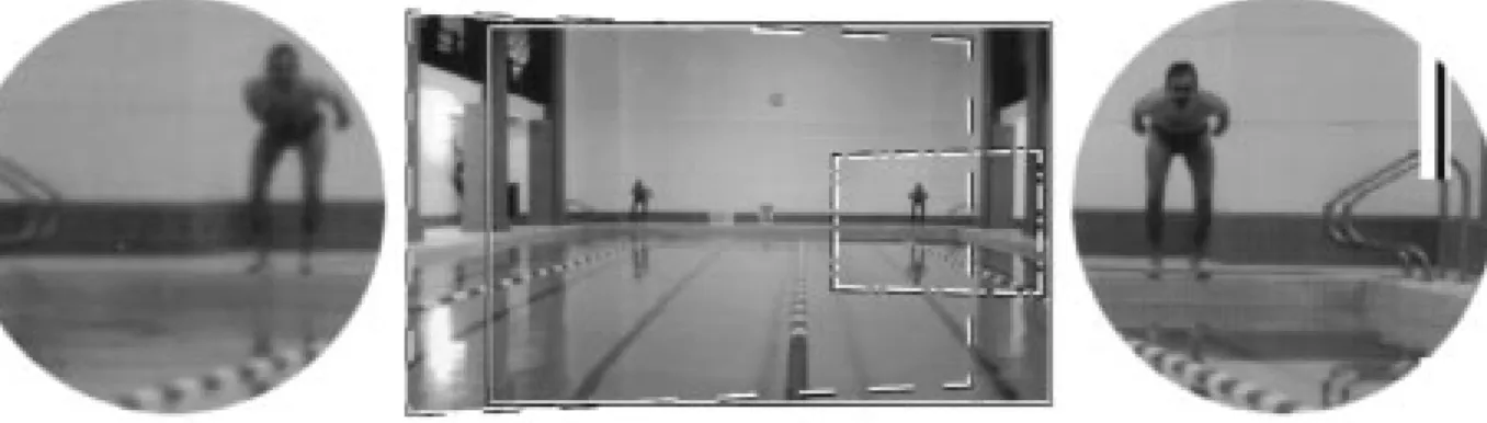
and example, how the new approach is more accurate and robust than previous approaches which relied on affine coordi-nate transformations, approximations to projective coordicoordi-nate transformations, and/or the finding of point correspondences between the images. The new techniques take as input two frames, and automatically output the eight parameters of the “exact” model, to properly register the frames. They do not require the tracking or correspondence of explicit features, yet are computationally easy to implement. Although the theory we present makes the typical assumptions of static scene and no parallax, we show that the new estimation techniques are robust to deviations from these assumptions. In particular, we apply the direct featureless projective parameter estimation approach to image resolution enhancement and compositing, illustrating its success on a variety of practical and difficult cases, including some that violate the nonparallax and static scene assumptions. An example image composite, made with featureless projective parameter estimation, is reproduced in Fig. 1, where the spatial extent of the image is increased by panning the camera while compositing (e.g., by making a panorama) and the spatial resolution is increased by zooming the camera and by combining overlapping frames.
II. BACKGROUND
Hundreds of papers have been published on the problems of motion estimation and frame alignment. (For review and comparison, see [1].) In this section we review the basic differences between coordinate transformations and emphasize the importance of using the “exact” eight-parameter projective coordinate transformation.
A. Coordinate Transformations
A coordinate transformation maps the image coordinates,
to a new set of coordinates, . The
approach to “finding the coordinate transformation” relies on assuming it will take one of the forms in Table I, and then estimating the parameters (two to 12 parameters depending on the model) in the chosen form. An illustration showing the effects possible with each of these forms is shown in Fig. 3.
The most common assumption (especially in motion esti-mation for coding, and optical flow for computer vision) is that the coordinate transformation between frames is trans-lation. Tekalp et al. [1] have applied this assumption to high-resolution image reconstruction. Although translation is the least constraining and simplest to implement of the seven coordinate transformations in Table I, it is poor at handling large changes due to camera zoom, rotation, pan, and tilt.
Fig. 1. Image composite made from three pictures (moving between two different locations) in a large room: One was taken looking straight ahead (outlined in a solid line), one was taken panning to the left (outlined in a dashed line), and the third was taken panning to the right with substantial zoom-in (outlined in a dot-dash line). The second two have undergone a coordinate transformation to put them into the same coordinates as the one outlined in a solid line (which we call the reference frame). This composite, made from NTSC-resolution images, occupies about 2000 pixels across and, in places, shows good detail down to the pixel level. Note increased sharpness in regions visited by the zooming-in, compared to other areas. (See magnified portions of composite at sides.) This composite only shows the result of combining three images, but in the final production, many more images were used, resulting in a high resolution full-color composite showing most of the room (figure reproduced from [6], courtesy of IS&T.).
TABLE I
IMAGE COORDINATETRANSFORMATIONSDISCUSSED INTHISPAPER
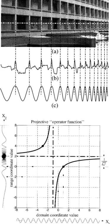
Zheng and Chellappa [3] considered the image registration problem using a subset of the affine model—translation, rota-tion, and scale. Other researchers [4], [5] have assumed affine motion (six parameters) between frames. For the assumptions of static scene and no parallax, the affine model exactly describes rotation about the optical axis of the camera, zoom of the camera, and pure shear, which the camera does not do, except in the limit as the lens focal length approaches infinity. The affine model cannot capture camera pan and tilt, and therefore cannot properly express the “keystoning” and “chirping” we see in the real world. (By “chirping” we mean the effect of increasing or decreasing spatial frequency with respect to spatial location, as illustrated in Fig. 2.) Conse-quently, the affine model attempts to fit the wrong parameters to these effects. Even though it has fewer parameters, we find that the affine model is more susceptible to noise because it lacks the correct degrees of freedom needed to properly track the actual image motion.
The eight-parameter projective model gives the desired eight parameters that exactly account for all possible zero-parallax camera motions; hence, there is an important need for a featureless estimator of these parameters. To the best of our knowledge, the only algorithms proposed to date for such an estimator are [6], and shortly after, [7]. In both of these, a computationally expensive nonlinear optimization method was presented. In [6], a direct method was also proposed. This direct method uses simple linear algebra, and is noniterative
insofar as methods such as Levenberg–Marquardt and the like are in no way required. The proposed method instead uses repetition with the correct law of composition on the projective group, going from one pyramid level to the next by application of the group’s law of composition. Because the parameters of the projective coordinate transformation had traditionally been thought to be mathematically and computationally too difficult to solve, most researchers have used the simpler affine model or other approximations to the projective model. Before we propose and demonstrate the featureless estimation of the parameters of the “exact” projective model, it is helpful to discuss some approximate models.
Going from first order (affine), to second order, gives the 12-parameter “biquadratic” model. This model properly captures both the chirping (change in spatial frequency with position) and converging lines (keystoning) effects associated with projective coordinate transformations, but does not constrain chirping and converging to work together (the example in Fig. 3 being chosen with zero convergence yet substantial chirping, illustrates this point). Despite its larger number of parameters, there is still considerable discrepancy between a projective coordinate transformation and the best-fit biquadratic coordinate transformation. Why stop at second order? Why not use a 20-parameter “bicubic model”? While an increase in the number of model parameters will result in a better fit, there is a tradeoff, where the model begins to fit noise. The physical camera model fits
(d)
Fig. 2. The “projective chirping” phenomenon. (a) Real-world object that exhibits periodicity generates a projection (image) with “chirp-ing”—“periodicity-in-perspective.” (b) Center raster of image. (c) Best-fit projective chirp of formsin f2[(ax+b)=(cx+1)]g. (d) Graphical depiction of exemplar 1-D projective coordinate transformation ofsin (2x1) into a “projective chirp” function,sin (2x2) = sin f2[(2x10 2)=(x1+ 1)]g.
The range coordinate as a function of the domain coordinate forms a rectangular hyperbola with asymptotes shifted to center at the vanishing
pointx1= 01=c = 01 and “exploding point,” x2= a=c = 2, and with
“chirpiness”c0 = c2=(bc 0 a) = 01=4.
exactly in the 8-parameter projective group; therefore, we know that “eight is enough.” Hence, it seems reasonable to have a preference for approximate models with exactly eight parameters.
The eight-parameter bilinear model is perhaps the most widely-used [8] in the fields of image processing, medical imaging, remote sensing, and computer graphics. This model is easily obtained from the biquadratic model by removing the four and terms. Although the resulting bilinear model captures the effect of converging lines, it completely fails to capture the effect of chirping.
The eight-parameter pseudoperspective model [9] and an eight-parameter “relative-projective” model both do, in fact, capture both the converging lines and the chirping of a projective coordinate transformation. The pseudoperspective model, for example, may be thought of as first, removal of two of the quadratic terms ( ), which results in a ten parameter model (the -chirp of [10]) and then constraining the four remaining quadratic parameters to have two degrees of freedom. These constraints force the “chirping effect” (captured by and ) and the “converging effect” (captured by and ) to work together in the “right” way to match, as closely as possible, the effect of a projective
coordinate transformation. By setting , the
chirping in the -direction is forced to correspond with the converging of parallel lines in the -direction (and likewise for the -direction).
Of course, the desired “exact” eight parameters come from the projective model, but they have been perceived as being notoriously difficult to estimate. The parameters for this model have been solved by Tsai and Huang [11], but their solution assumed that features had been identified in the two frames, along with their correspondences. The main contribution of this paper is a simple featureless means of automatically solving for these eight parameters.
Other researchers have looked at projective estimation in the context of obtaining 3-D models. Faugeras and Lustman [12], Shashua and Navab [13], and Sawhney [14] have considered the problem of estimating the projective parameters while computing the motion of a rigid planar patch, as part of a larger problem of finding 3-D motion and structure using parallax relative to an arbitrary plane in the scene. Kumar et al. [15] have also suggested registering frames of video by computing the flow along the epipolar lines, for which there is also an initial step of calculating the gross camera movement assuming no parallax. However, these methods have relied on feature correspondences, and were aimed at 3-D scene modeling. Our focus is not on recovering the 3-D scene model, but on aligning two-dimensional (2-D) images of 3-D scenes. Feature correspondences greatly simplify the problem; however, they also have many problems. The focus of this paper is simple featureless approaches to estimating the projective coordinate transformation between image pairs.
B. Camera Motion: Common Assumptions and Terminology Two assumptions are typical in this area of research. The first assumption is that the scene is constant—changes of scene content and lighting are small between frames. The second assumption is that of an ideal pinhole camera—implying unlimited depth of field with everything in focus (infinite resolution) and implying that straight lines map to straight
TABLE II
THETWO“NO PARALLAX” CASES FOR ASTATICSCENE
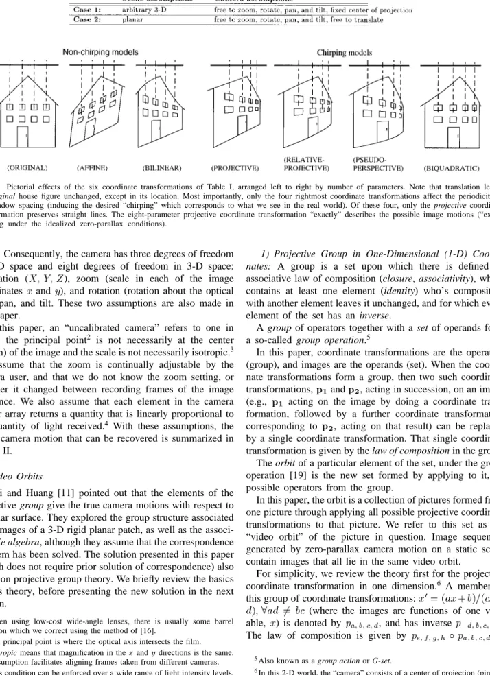
Fig. 3. Pictorial effects of the six coordinate transformations of Table I, arranged left to right by number of parameters. Note that translation leaves the original house figure unchanged, except in its location. Most importantly, only the four rightmost coordinate transformations affect the periodicity of the window spacing (inducing the desired “chirping” which corresponds to what we see in the real world). Of these four, only the projective coordinate transformation preserves straight lines. The eight-parameter projective coordinate transformation “exactly” describes the possible image motions (“exact” meaning under the idealized zero-parallax conditions).
lines.1Consequently, the camera has three degrees of freedom
in 2-D space and eight degrees of freedom in 3-D space: translation ( ), zoom (scale in each of the image coordinates and ), and rotation (rotation about the optical axis, pan, and tilt. These two assumptions are also made in this paper.
In this paper, an “uncalibrated camera” refers to one in which the principal point2 is not necessarily at the center (origin) of the image and the scale is not necessarily isotropic.3
We assume that the zoom is continually adjustable by the camera user, and that we do not know the zoom setting, or whether it changed between recording frames of the image sequence. We also assume that each element in the camera sensor array returns a quantity that is linearly proportional to the quantity of light received.4 With these assumptions, the
exact camera motion that can be recovered is summarized in Table II.
C. Video Orbits
Tsai and Huang [11] pointed out that the elements of the projective group give the true camera motions with respect to a planar surface. They explored the group structure associated with images of a 3-D rigid planar patch, as well as the associ-ated lie algebra, although they assume that the correspondence problem has been solved. The solution presented in this paper (which does not require prior solution of correspondence) also relies on projective group theory. We briefly review the basics of this theory, before presenting the new solution in the next section.
1When using low-cost wide-angle lenses, there is usually some barrel
distortion which we correct using the method of [16].
2The principal point is where the optical axis intersects the film. 3Isotropic means that magnification in thex and y directions is the same.
Our assumption facilitates aligning frames taken from different cameras.
4This condition can be enforced over a wide range of light intensity levels,
by using the Wyckoff principle [17], [18].
1) Projective Group in One-Dimensional (1-D) Coordi-nates: A group is a set upon which there is defined an associative law of composition (closure, associativity), which contains at least one element (identity) who’s composition with another element leaves it unchanged, and for which every element of the set has an inverse.
A group of operators together with a set of operands form a so-called group operation.5
In this paper, coordinate transformations are the operators (group), and images are the operands (set). When the coordi-nate transformations form a group, then two such coordicoordi-nate transformations, and , acting in succession, on an image (e.g., acting on the image by doing a coordinate trans-formation, followed by a further coordinate transformation corresponding to , acting on that result) can be replaced by a single coordinate transformation. That single coordinate transformation is given by the law of composition in the group. The orbit of a particular element of the set, under the group operation [19] is the new set formed by applying to it, all possible operators from the group.
In this paper, the orbit is a collection of pictures formed from one picture through applying all possible projective coordinate transformations to that picture. We refer to this set as the “video orbit” of the picture in question. Image sequences generated by zero-parallax camera motion on a static scene contain images that all lie in the same video orbit.
For simplicity, we review the theory first for the projective coordinate transformation in one dimension.6 A member of
this group of coordinate transformations:
(where the images are functions of one
vari-able, ) is denoted by , and has inverse .
The law of composition is given by
5Also known as a group action or G-set.
6In this 2-D world, the “camera” consists of a center of projection (pinhole
. In almost all practical engineering applications, , so we will divide through by , and
denote the coordinate transformation by
. When and , the projective group
becomes the affine group of coordinate transformations, and when and , it becomes the group of translations.
Of the coordinate transformations presented in the previous section, only the projective, affine, and translation operations form groups.
The equivalent two cases of Table II for this hypothetical “flatland” world of 2-D objects with 1-D pictures correspond to the following. In the first case, a camera is at a fixed location, and free to zoom and pan. In the second case, a camera is free to translate, zoom, and pan, but the imaged object must be flat (i.e., lie on a straight line in the plane). The resulting two (1-D) frames taken by the camera are related by the coordinate transformation from to , given by [20] as
(1)
where , and
, is the location of the singularity in the domain. We should mention that , the degree of perspective, has been given the interpretation of a chirp-rate [20].
The coordinate transformations of (1) form a group oper-ation. This result, and the proof of this group’s isomorphism to the group corresponding to nonsingular projections of a flat object are given in [21].
2) Projective Group in 2-D Coordinates: The theory for the projective, affine, and translation groups also holds for the familiar 2-D images taken of the 3-D world. The “video orbit” of a given 2-D frame is defined to be the set of all images that can be produced by applying operators from the 2-D projective group to the given image. Hence, we restate the coordinate transformation problem: Given a set of images that lie in the same orbit of the group, we wish to find for each image pair, that operator in the group that takes one image to the other image.
If two frames, say, and , are in the same orbit, then there is an group operation such that the mean-squared error (MSE) between and is zero. In practice, however, we find which element of the group takes one image “nearest” the other, for there will be a certain amount of parallax, noise, interpolation error, edge effects, changes in lighting, depth of focus, etc. Fig. 4 illustrates the operator acting on frame , to move it nearest to frame . (This figure does not, however, reveal the precise shape of the orbit, which occupies an eight-dimensional space.)
Summarizing, the eight-parameter projective group captures the exact coordinate transformation between pictures taken under the two cases of Table II. The primary assumptions in these cases are that of no parallax, and of a static scene. Because the eight-parameter projective model is “exact,” it is theoretically the right model to use for estimating the coordinate transformation. Examples presented in this paper
demonstrate that it also performs better in practice than the other proposed models.
III. FRAMEWORK: MOTION PARAMETER
ESTIMATION AND OPTICAL FLOW
To lay the framework for our new results, we will re-view existing methods of parameter estimation for coordinate transformations. This framework will apply to both existing methods as well as our new methods. The purpose of this review is to bring together a variety of methods that appear quite different, but which actually can be described in a more unified framework, which we present here.
The framework we give breaks existing methods into two categories: feature-based, and featureless. Of the featureless methods, we consider two subcategories: i) methods based on minimizing MSE (generalized correlation, direct nonlin-ear optimization) and ii) methods based on spatiotemporal derivatives and optical flow. Note that variations such as multiscale have been omitted from these categories; multiscale analysis can be applied to any of them. The new algorithms we develop in this paper (with final form given in Section IV) are featureless, and based on (multiscale if desired) spatiotemporal derivatives.
Some of the descriptions of methods below will be pre-sented for hypothetical 1-D images taken of 2-D “scenes” or “objects.” This simplification yields a clearer comparison of the estimation methods. The new theory and applications will be presented subsequently for 2-D images taken of 3-D scenes or objects.
A. Feature-Based Methods
Feature-based methods [22], [23] assume that point cor-respondences in both images are available. In the projective case, given at least three correspondences between point pairs in the two 1-D images, we will find the element,
that maps the second image into the first. Let be the points in one image, and let be the corresponding points in the other image. Then
. Rearranging yields ,
so that , and can be found by solving linear
equations in three unknowns, as follows:
(2) using least squares if there are more than three correspondence points. The extension from 1-D “images” to 2-D images is conceptually identical; for the affine and projective models, the minimum number of correspondence points needed in 2-D is three and four, respectively.
A major difficulty with feature-based methods is finding the features. Good features are often hand-selected, or computed, possibly with some degree of human intervention [24]. A second problem with features is their sensitivity to noise and occlusion. Even if reliable features exist between frames (e.g., line markings on a playing field in a football video, see Section V-B), these features may be subject to signal noise and occlusion (e.g., running football players blocking
(a) (b)
Fig. 4. Video orbits. (a) The orbit of frame 1 is the set of all images that can be produced by acting on frame 1 with any element of the operator group. Assuming that frames 1 and 2 are from the same scene, frame 2 will be close to one of the possible projective coordinate transformations of frame 1. In other words, frame 2 “lies near the orbit of” frame 1. (b) By bringing frame 2 along its orbit, we can determine how closely the two orbits come together at frame 1.
a feature). The emphasis in the rest of this paper will be on robust featureless methods.
B. Featureless Methods Based on Generalized Cross-Correlation
The purpose of this section is for completeness: We will consider first what is perhaps the most obvious approach (generalized cross-correlation in 8-D parameter space) in order to motivate a different approach provided in Section III-C, the motivation arising from ease of implementation and simplicity of computation.
Cross-correlation of two frames is a featureless method of recovering translation model parameters. Affine and projective parameters can also be recovered using generalized forms of cross-correlation.
Generalized cross-correlation is based on an inner-product formulation which establishes a similarity metric between two functions, say, and , where is an approximately coordinate-transformed version of , but the parameters of the coordinate transformation, are unknown.7 We can find, by
exhaustive search (applying all possible operators, , to ), the “best” as the one that maximizes the inner product
(3)
where we have normalized the energy of each coordinate-transformed before making the comparison. Equivalently, instead of maximizing a similarity metric, we can minimize some distance metric, such as MSE, given by
. Solving (3) has an advantage over finding MSE when one image is not only a coordinate-transformed version of the other, but is also an amplitude-scaled version, as generally happens when there is an automatic gain control or an automatic iris in the camera.
In one dimension, the orbit of an image under the affine group operation is a family of wavelets, while the orbit of an image under the projective group of coordinate transformations
7In the presence of additive white Gaussian noise, this method, also
known as “matched filtering,” leads to a maximum likelihood estimate of the parameters [25].
is a family of “projective chirplets” [26],8the objective
func-tion (3) being the cross-chirplet transform. A computafunc-tionally efficient algorithm for the cross-wavelet transform has recently been presented [29]. (See [30] for a good review on wavelet-based estimation of affine coordinate transformations.)
Adaptive variants of the chirplet transforms have been previously reported in the literature [31]. However, there are still many problems with the adaptive chirplet approach; thus, for the remainder of this paper, we consider featureless methods based on spatiotemporal derivatives.
C. Featureless Methods Based on Spatio-Temporal Derivatives 1) Optical Flow (“Translation Flow”): When the change from one image to another is small, optical flow [32] may be used. In one dimension, the traditional optical flow formulation assumes each point in frame is a translated version of the corresponding point in frame , and that and are chosen in the ratio , the translational flow velocity of the point in question. The image brightness
is described by
(4) where is the translational flow velocity of the point in the case of pure translation, where is constant across the entire image. More generally, though, a pair of 1-D images are related by a quantity, at each point in one of the images. Expanding the right hand side of (4) in a Taylor series, and canceling zeroth-order terms gives the well-known optical
flow equation: , where and are
the spatial and temporal derivatives, respectively, and denotes higher order terms. Typically, the higher order terms are neglected, giving the expression for the optical flow at each point in one of the two images
(5) 2) Weighing the Difference Between “Affine Fit” and “Affine Flow”: A comparison between two similar ap-proaches is presented, in the familiar and obvious realm of linear regression versus direct affine estimation, highlighting the obvious differences between the two approaches. This difference, in weighting, motivates new weighting changes, which will later simplify implementations pertaining to the new methods.
Given the optical flow between two images, and , we wish to find the coordinate transformation to apply to to register it with . We now describe two approaches based on the affine model:9 i) finding the optical flow at every point,
and then fitting this flow with an affine model (“affine fit”), and ii) rewriting the optical flow equation in terms of an affine (not translation) motion model (“affine flow”).
Wang and Adelson have proposed fitting an affine model to the optical flow field [33] between two 2-D images. We briefly
8Symplectomorphisms of the time-frequency plane [27], [28] have been
applied to signal analysis, giving rise to the so-called q-chirplet [26], which differs from the projective chirplet discussed here.
9The 1-D affine model is a simple yet sufficiently interesting (non-Abelian)
examine their approach with 1-D images; the reduction in dimensions simplifies analysis and comparison to affine flow. Denote coordinates in the original image, , by , and in the new image, , by . Suppose that is a dilated and translated
version of , so for every corresponding pair
. Equivalently, the affine model of velocity [normalizing
], , is given by . We can
expect a discrepancy between the flow velocity, , and the model velocity, , due to either errors in the flow calculation, or to errors in the affine model assumption, so we apply linear regression to get the best least-squares fit by minimizing
(6) The constants and that minimize over the entire patch are found by differentiating (6), and setting the derivatives to zero. This results in what we call the affine fit equations
(7)
Alternatively, the affine coordinate transformation may be directly incorporated into the brightness change constraint (4). Bergen et al. [34] have proposed this method, which we will call affine flow, to distinguish it from the “affine fit” model of Wang and Adelson (7). Let us show how affine flow and affine fit are related. Substituting directly into (5) in place of and summing the squared error
(8) over the whole image, differentiating, and equating the result to zero, gives a linear solution for both and , as follows:
(9)
To see how this result compares to the affine fit, we rewrite (6)
(10) and observe, comparing (8) and (10) that affine flow is equivalent to a weighted least-squares fit, where the weighting is given by . Thus, the affine flow method tends to put more emphasis on areas of the image that are spatially varying than does the affine fit method. Of course, one is free to separately choose the weighting for each method in such a way that affine fit and affine flow methods both give the same result. Both our intuition and our practical experience tends to favor the affine flow weighting, but, more generally, perhaps we should ask, what is the best weighting? Lucas and Kanade [35], among others, have considered weighting issues, though
the rather obvious difference in weighting between fit and flow does not appear to have been pointed out previously in the literature. The fact that the two approaches provide similar results, yet have drastically different weightings, suggests that we can exploit the choice of weighting. In particular, we will observe in Section III-C3 that we can select a weighting that makes the implementation easier.
Another approach to the affine fit involves computation of the optical flow field using the multiscale iterative method of Lucas and Kanade, and then fitting to the affine model. An analogous variant of the affine flow method involves multiscale iteration as well, but in this case the iteration and multiscale hierarchy are incorporated directly into the affine estimator [34]. With the addition of multiscale analysis, the “fit” and “flow” methods differ in additional respects beyond just the weighting. Our intuition and experience indicates that the direct multiscale affine flow performs better than the affine fit to the multiscale flow. Multiscale optical flow makes the assumption that blocks of the image are moving with pure translational motion, and then, paradoxically, the affine fit refutes this pure-translation assumption. However, fit provides some utility over flow when it is desired to segment the image into regions undergoing different motions [36], or to gain robustness by rejecting portions of the image not obeying the assumed model.
3) “Projective Fit” and “Projective Flow”—New Tech-niques: Analogous to the affine fit and affine flow of the previous section, we now propose the two new methods: “projective fit” and “projective flow.” For the 1-D affine coordinate transformation, the graph of the range coordinate as a function of the domain coordinate is a straight line; for the projective coordinate transformation, the graph of the range coordinate as a function of the domain coordinate is a rectangular hyperbola [Fig. 2(d)]. The affine fit case used linear regression; however, in the projective case we use hyperbolic regression. Consider the flow velocity given by (5) and the model velocity
(11) and minimize the sum of the squared difference, as was done in (6), to
(12)
As discussed earlier, the calculation can be simplified by judicious alteration of the weighting, in particular, multiplying each term of the summation (12) by , and solving, gives
(13)
where the regressor is .
For projective flow, we substitute
into (8). Again, weighting by gives
(the subscript denotes weighting has taken place) resulting in a linear system of equations for the parameters
(15)
where . Again, to show
the difference in the weighting between projective flow and projective fit, we can rewrite (15)
(16) where is that defined in (13).
4) The Unweighted Projectivity Estimator: If we do not wish to apply the ad hoc weighting scheme, we may still estimate the parameters of projectivity in a simple manner, still based on solving a linear system of equations. To do this, we write the Taylor series of
(17) and use the first three terms, obtaining enough degrees of freedom to account for the three parameters being estimated. Letting
, and ,
and differentiating with respect to each of the three parameters of , setting the derivatives equal to zero, and verifying with the second derivatives, gives the following linear system of equations for “unweighted projective flow”:
(18)
In Section IV, we will extend this derivation to 2-D images.
IV. MULTISCALEIMPLEMENTATIONS INTWO DIMENSIONS
In the previous section, two new techniques, projective-fit and projective-flow, were proposed. Now we describe these algorithms for 2-D images. The brightness constancy constraint equation for 2-D images [32] that gives the flow velocity components in the and directions, analogous to (5) is
(19) As is well known, the optical flow field in two dimensions is underconstrained.10 The model of pure translation at every
point has two parameters, but there is only one (19) to solve, thus it is common practice to compute the optical flow over some neighborhood, which must be at least two pixels, but is generally taken over a small block, 3 3, 5 5, or sometimes larger (e.g., the entire image, as in this paper).
10Optical flow in one dimension did not suffer from this problem.
Our task is not to deal with the 2-D translational flow, but with the 2-D projected flow, estimating the eight parameters in the coordinate transformation
(20) The desired eight scalar parameters are denoted by
, and .
Analogous to (10), we have, in the 2-D case
(21) Where the sum can be weighted,as it was in the 1-D case, as (22) Differentiating with respect to the free parameters , and , and setting the result to zero gives a linear solution, we get
(23) where
. A. “Unweighted Projective Flow”
As with the 1-D images, we make similar assumptions in expanding (20) in its own Taylor series, analogous to (17). If we take the Taylor series up to second-order terms, we obtain the biquadratic model mentioned in Section II-A. As mentioned in Section II-A, by appropriately constraining the 12 parameters of the biquadratic model, we obtain a variety of eight-parameter approximate models. In our algorithms for es-timating the “exact unweighted” projective group parameters, we use one of these approximate models in an intermediate step.11
The Taylor series for the bilinear case gives
(24) Incorporating these into the flow criteria yields a simple set of eight linear equations in eight unknowns, as follows:
(25)
where .
For the relative-projective model, is given by
(26) and for the pseudoperspective model, is given by
(27)
11Use of an approximate model that does not capture chirping or preserve
straight lines can still lead to the true projective parameters as long as the model captures at least eight degrees of freedom.
In order to see how well the model describes the coordinate transformation between two images, say, and , one might warp12 to , using the estimated motion model, and then
compute some quantity that indicates how different the resam-pled version of is from . The MSE between the reference image and the warped image might serve as a good measure of similarity. However, since we are really interested in how the exact model describes the coordinate transformation, we assess the goodness of fit by first relating the parameters of the approximate model to the exact model, and then find the MSE between the reference image and the comparison image after applying the coordinate transformation of the exact model. A method of finding the parameters of the exact model, given the approximate model, is presented in Section IV-A1.
1) “Four-Point Method” for Relating Approximate Model to Exact Model: Any of the approximations above, after being related to the exact projective model, tend to behave well in the
neighborhood of the identity . In
one-dimension, we explicitly expanded the model Taylor series about the identity; here, although we do not explicitly do this, we shall assume that the terms of the Taylor series of the model correspond to those taken about the identity. In the 1-D case, we solve the three linear equations in three unknowns to estimate the parameters of the approximate motion model, and then relate the terms in this Taylor series to the exact parameters, , , and (which involves solving another set of three equations in three unknowns, the second set being nonlinear, although very easy to solve).
In the extension to two dimensions, the estimate step is straightforward, but the relate step is more difficult, because we now have eight nonlinear equations in eight unknowns, relating the terms in the Taylor series of the approximate model to the desired exact model parameters. Instead of solving these equations directly, we now propose the following simple procedure for relating the parameters of the approximate model to those of the exact model, which we call the “four-point method”.
1) Select four ordered pairs (e.g., the four corners of the bounding box containing the region under analysis, or the four corners of the image if the whole image is under analysis). Here suppose, for simplicity, that these points are the corners of the unit {square:
.
2) Apply the coordinate transformation using the Taylor series for the approximate model [e.g., (24)] to these
points: .
3) Finally, the correspondences between and are treated just like features. This results in four easy to solve linear equations
(28)
where . This results in the exact eight
parameters, .
12The term warp is appropriate here, since the approximate model does not
preserve straight lines.
Fig. 5. Method of computation of eight parametersp between two images from the same pyramid level,g and h. The approximate model parameters q are related to the exact model parametersp in a feedback system.
We remind the reader that the four corners are not feature correspondences as used in the feature-based methods of Section III-A, but rather are used so that the two featureless models (approximate and exact) can be related to one another. It is important to realize the full benefit of finding the exact parameters. While the “approximate model” is sufficient for small deviations from the identity, it is not adequate to describe large changes in perspective. However, if we use it to track small changes incrementally, and each time relate these small changes to the exact model (20), then we can accumulate these small changes using the law of composition afforded by the group structure. This is an especially favorable contribution of the group framework. For example, with a video sequence, we can accommodate very large accumulated changes in perspective in this manner. The problems with cumulative error can be eliminated, for the most part, by constantly propagating forward the true values, computing the residual using the approximate model, and each time relating this to the exact model to obtain a goodness-of-fit estimate.
2) Overview of Algorithm for Unweighted Projective Flow: Below is an outline of the algorithm; details of each step are in subsequent sections.
Frames from an image sequence are compared pairwise to test whether or not they lie in the same orbit:
1) A Gaussian pyramid of three or four levels is constructed for each frame in the sequence.
2) The parameters are estimated at the top of the pyramid, between the two lowest-resolution images of a frame pair, and , using the iterative method depicted in Fig. 5.
3) The estimated is applied to the next higher-resolution (finer) image in the pyramid, , to make the two images at that level of the pyramid nearly congruent before estimating the between them.
4) The process continues down the pyramid until the highest-resolution image in the pyramid is reached. B. Multiscale Iterative Implementation
The Taylor-series formulations we have used implicitly assume smoothness; the performance is improved if the images are blurred before estimation. To accomplish this, we do not downsample critically after lowpass filtering in the pyramid. However, after estimation, we use the original (unblurred) images when applying the final coordinate transformation.
The strategy we present differs from the multiscale iterative (affine) strategy of Bergen et al., in one important respect beyond simply an increase from six to eight parameters. The
difference is the fact that we have two motion models, the “ex-act motion model” (20) and the “approximate motion model,” namely the Taylor series approximation to the motion model itself. The approximate motion model is used to repetitively converge to the exact motion model, using the algebraic law of composition afforded by the exact projective group model. In this strategy, the exact parameters are determined at each level of the pyramid, and passed to the next level. The steps involved are summarized schematically in Fig. 5, and described below.
1) Initialize: Set and set to the identity
operator.
2) Repeat ( ):
a) Estimate the eight or more terms of the approximate model between two image frames, and . This results in approximate model parameters
b) Relate the approximate parameters to the ex-act parameters using the “four point method.” The resulting exact parameters are .
c) Resample: Apply the law of composition to accumu-late the effect of the ’s. Denote these composite
parameters by . Then set
. (This should have nearly the same effect as applying to , except that it will avoid additional interpolation and antialiasing errors you would get by resampling an already resampled image [8]).
Repeat until either the error between and falls below a threshold, or until some maximum number of iterations is achieved. After the first iteration, the parameters tend to be near the identity since they account for the residual between the “perspective-corrected” image and the “true” image . We find that only two or three iterations are usually needed for frames from nearly the same orbit.
A rectangular image assumes the shape of an arbitrary quadrilateral when it undergoes a projective coordinate trans-formation. In coding the algorithm, we pad the undefined portions with the quantity NaN, a standard IEEE arithmetic value, so that any calculations involving these values auto-matically inherit NaN without slowing down the computations. The algorithm (in Matlab on an HP 735) takes about 6 s per repetition for a pair of 320 240 images.
C. Exploiting Commutativity for Parameter Estimation There is a fundamental uncertainty [37] involved in the simultaneous estimation of parameters of a noncommutative group, akin to the Heisenberg uncertainty relation of quan-tum mechanics. In contrast, for a commutative13 group (in the absence of noise), we can obtain the exact coordinate transformation.
Segman [38] considered the problem of estimating the parameters of a commutative group of coordinate transforma-tions, in particular, the parameters of the affine group [39]. His
13A commutative (or Abelian) group is one in which elements of the group
commute, for example, translation along thex-axis commutes with translation along they-axis, so the 2-D translation group is commutative.
work also deals with noncommutative groups, in particular, in the incorporation of scale in the Heisenberg group.14
Estimating the parameters of a commutative group is com-putationally efficient, e.g., through the use of Fourier cross-spectra [41]. We exploit this commutativity for estimating the parameters of the noncommutative 2-D projective group by first estimating the parameters that commute. For example, we improve performance if we first estimate the two pa-rameters of translation, correct for the translation, and then proceed to estimate the eight projective parameters. We can also simultaneously estimate both the isotropic-zoom and the rotation about the optical axis by applying a log-polar coordinate transformation followed by a translation estimator. This process may also be achieved by a direct application of the Fourier–Mellin transform [42]. Similarly, if the only difference between and is a camera pan, then the pan may be estimated through a coordinate transformation to cylindrical coordinates, followed by a translation estimator.
In practice, we run through the following “commutative ini-tialization” before estimating the parameters of the projective group of coordinate transformations.
1) Assume that is merely a translated version of . a) Estimate this translation using the method of Girod
[41].
b) Shift by the amount indicated by this estimate. c) Compute the MSE between the shifted and , and
compare to the original MSE before shifting. d) If an improvement has resulted, use the shifted
from now on.
2) Assume that is merely a rotated and isotropically zoomed version of .
a) Estimate the two parameters of this coordinate trans-formation.
b) Apply these parameters to .
c) If an improvement has resulted, use the coordinate-transformed (rotated and scaled) from now on. 3) Assume that is merely an “x-chirped” (panned) version
of , and, similarly, “x-dechirp” . If an improvement results, use the “x-dechirped” from now on. Repeat for (tilt.)
Compensating for one step may cause a change in choice of an earlier step. Thus, it might seem desirable to run through the commutative estimates iteratively. However, our experience on lots of real video indicates that a single pass usually suffices, and in particular, will catch frequent situations where there is a pure zoom, a pure pan, a pure tilt, etc., both saving the rest of the algorithm computational effort, as well as accounting for simple coordinate transformations such as when one image is an upside-down version of the other. (Any of these pure cases corresponds to a single parameter group, which is commutative.) Without the “commutative initialization”step, these parameter estimation algorithms are prone to get caught in local optima, and thus never converge to the global optimum.
14While the Heisenberg group deals with translation and
frequency-translation (modulation), some of the concepts could be carried over to other more relevant group structures.
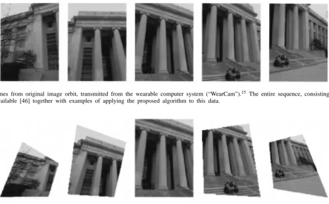
Fig. 6. Frames from original image orbit, transmitted from the wearable computer system (“WearCam”).15 The entire sequence, consisting of 20 color frames, is available [46] together with examples of applying the proposed algorithm to this data.
Fig. 7. Frames from original image video orbit after a coordinate transformation to move them along the orbit to the reference frame (c). The coordinate-transformed images are alike except for the region over which they are defined. Note that the regions are not parallelograms; thus, methods based on the affine model fail.
V. PERFORMANCE AND APPLICATIONS
Fig. 6 shows some frames from a typical image sequence. Fig. 7 shows the same frames brought into the coordinate system of frame (c), that is, the middle frame was chosen as the reference frame.
Given that we have established a means of estimating the projective coordinate transformation between any pair of images, there are two basic methods we use for finding the coordinate transformations between all pairs of a longer image sequence. Because of the group structure of the projective coordinate transformations, it suffices to arbitrarily select one frame and find the coordinate transformation between every other frame and this frame. The two basic methods are described below.
1) Differential Parameter Estimation: The coordinate transformations between successive pairs of images,
, estimated.
2) Cumulative Parameter Estimation: The coordinate transformation between each image and the refer-ence image is estimated directly. Without loss of generality, select frame zero ( ) as the reference frame and denote these coordinate transformations as
.
Theoretically, these two methods are equivalent:
differential method
cumulative method (29)
However, in practice, the two methods differ for the fol-lowing two reasons.
15Note that WearCam [47] is mounted sideways so that it can “paint” out
the image canvas with a wider “brush,” when sweeping across for a panorama.
1) Cumulative Error: In practice, the estimated coordinate transformations between pairs of images register them only approximately, due to violations of the assumptions (e.g., objects moving in the scene, center of projection not fixed, camera swings around to bright window and automatic iris closes, etc.). When a large number of estimated parameters are composed, cumulative error sets in.
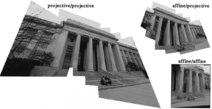
2) Finite Spatial Extent of Image Plane: Theoretically, the images extend infinitely in all directions, but, in practice, images are cropped to a rectangular bounding box. Therefore, a given pair of images (especially if they are far from adjacent in the orbit) may not overlap at all; hence, it is not possible to estimate the parameters of the coordinate transformation using those two frames. The frames of Fig. 6 were brought into register using the dif-ferential parameter estimation, and “cemented” together seam-lessly on a common canvas. “Cementing” involves piecing the frames together, for example, by median, mean, or trimmed mean, or combining on a subpixel grid [21]. (Trimmed mean was used here, but the particular method made little visible dif-ference.) Fig. 8 shows this result (projective/projective), with a comparison to two nonprojective cases. The first comparison is to affine/affine where affine parameters were estimated (also multiscale) and used for the coordinate transformation. The second comparison, affine/projective, uses the six affine parameters found by estimating the eight projective parameters and ignoring the two chirp parameters (which capture the essence of tilt and pan). These six parameters are more accurate than those obtained using the affine estimation, as the affine estimation tries to fit its shear parameters to the camera pan and tilt. In other words, the affine estimation does worse
Fig. 8. Frames of Fig. 7 “cemented” together on single image “canvas,” with comparison of affine and projective models. Note the good registration and nice appearance of the projective/projective image despite the noise in the amateur television receiver, wind-blown trees, and the fact that the rotation of the camera was not actually about its center of projection. Note also that the affine model fails to properly estimate the motion parameters (affine/affine), and even if the “exact” projective model is used to estimate the affine parameters, there is no affine coordinate transformation that will properly register all of the image frames.
Fig. 9. Hewlett-Packard Claire image sequence, which violates the assumptions of the model (the camera location was not fixed, and the scene was not completely static). Images appear in TV raster-scan order.
than the six affine parameters within the projective estimation. The affine coordinate transform is finally applied, giving the image shown. Note that the coordinate-transformed frames in the affine case are parallelograms.
A. Subcomposites and the Support Matrix
The following two situations have so far been dealt with. 1) Camera movement is small, so that any pair of frames
chosen from the video orbit have a substantial amount of overlap when expressed in a common coordinate system. (Use differential parameter estimation.)
2) Camera movement is monotonic, so that any errors that accumulate along the registered sequence are not particularly noticeable. (Use cumulative parameter esti-mation.)
In the example of Fig. 8, any cumulative errors are not particularly noticeable because the camera motion is progres-sive, that is, it does not reverse direction or loop around on itself. Now let us look at an example where the camera motion loops back on itself and small errors, due to violations of the assumptions (fixed camera location and static scene), accumulate.
Consider the image sequence shown in Fig. 9. The com-posite arising from bringing these 16 image frames into the coordinates of the first frame exhibited somewhat poor registration due to cumulative error; we use this sequence to illustrate the importance of subcomposites.
The “differential support matrix,”15 for which the entry tells us how much frame overlaps with frame when expressed in the coordinates of frame , for the sequence of Fig. 9 appears in Fig. 10.
Examining the support matrix, and the mean-squared error estimates, the local maxima of the support matrix correspond to the local minima of the mean-squared error estimates,
sug-gesting the subcomposites16: ,
and . It is important to note that when the
error is low, if the support is also low, the error estimate might not be valid. For example, if the two images overlap in only one pixel, then even if the error estimate is zero (e.g., perhaps
15The “differential support matrix” is not necessarily symmetric, while the
“cumulative support matrix” for which the entryqm; n tells us how much framen overlaps with frame m when expressed in the coordinates of frame 0 (reference frame) is symmetric.
16Researchers at Sarnoff also consider the use of subcomposites, and refer
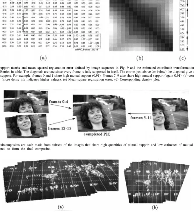
Fig. 10. Support matrix and mean-squared registration error defined by image sequence in Fig. 9 and the estimated coordinate transformations between images. (a) Entries in table. The diagonals are one since every frame is fully supported in itself. The entries just above (or below) the diagonal give the amount of pairwise support. For example, frames 0 and 1 share high mutual support (0.91). Frames 7–9 also share high mutual support (again 0.91). (b) corresponding
density plot (more dense ink indicates higher values). (c) Mean-square registration error. (d) Corresponding density plot.
Fig. 11. Subcomposites are each made from subsets of the images that share high quantities of mutual support and low estimates of mutual error, and then combined to form the final composite.
Fig. 12. Image composite made from 16 video frames taken from a television broadcast sporting event. Note the “Edgertonian” appearance, as each player traces out a stroboscopic-like path. The proposed method works robustly, despite the movement of players on the field. (a) Images are expressed in the coordinates of the first frame. (b) Images are expressed in a new useful coordinate system corresponding to none of the original frames. Note the slight distortion, due to the fact that football fields are not perfectly flat, but, rather, are raised slightly in the center.
that pixel has a value of 255 in both images), the alignment is not likely good.
The selected subcomposites appear in Fig. 11. Estimating the coordinate transformation between these subcomposites, and putting them together into a common frame of reference results in a composite (Fig. 11) about 1200 pixels across, where the image is sharp despite the fact that the person in the picture was moving slightly and the camera operator was also moving (violating the assumptions of both static scene and fixed center of projection).
B. Flat Subject Matter and Alternate Coordinates
Many sports such as football or soccer are played on a nearly flat field that forms a rigid planar patch over which the analysis may be conducted. After each of the frames undergoes the appropriate coordinate transformation to bring it into the same coordinate system as the reference frame, the sequence can be played back showing only the players (and the image boundaries) moving. Markings on the field (such as numbers and lines) remain at a fixed location, which makes subsequent
analysis and summary of the video content easier. This data makes a good test case for the algorithms because the video was noisy and the players caused the assumption of static scene to be violated.
Despite the players moving in the video, the proposed method successfully registers all of the images in the orbit, mapping them into a single high-resolution image composite of the entire playing field. Fig. 12(a) shows 16 frames of video from a football game combined into a single image composite, expressed in the coordinates of the first image in the sequence. The choice of coordinate system was arbitrary, and any of the images could have been chosen as the reference frame. In fact, a coordinate system other than one chosen from the input images could also be used. In particular, a coordinate system where parallel lines never meet, and periodic structures are “dechirped” [see Fig. 12(b)] lends itself well to machine vision and player-tracking algorithms [45]. Even if the entire playing field was never visible in any one image, collectively, the video from an entire game will likely reveal every square yard of playing surface at one time or another, hence enabling us to make a composite of the entire playing surface.
VI. CONCLUSIONS
We proposed and demonstrated featureless estimation of the projective coordinate transformation between two images. Not just one method, but various methods were proposed, among these, projective fit and projective flow, which estimate the projective (homographic) coordinate transformation between pairs of images, taken with a camera that is free to pan, tilt, rotate about its optical axis, and zoom. The new approach was also formulated and demonstrated within a multiscale iterative framework. Applications to seamlessly combining images in or near the same orbit of the projective group of coordinate transformations were also presented. The proposed approach solves for the eight parameters of the “exact” model (the projective group of coordinate transformations), is fully automatic, and converges quickly. The approach was also explored together with the use of subcomposites, useful when the camera motion loops back on itself.
The proposed method was found to work well on image data collected from both good-quality and poor-quality video under a wide variety of conditions (sunny, cloudy, day, night). It has been tested with a head-mounted wireless video camera, and performs successfully even in the presence of noise, interference, scene motion (such as people walking through the scene), lighting fluctuations, and parallax (due to movements of the wearer’s head). It remains to be shown which variant of the proposed approach is optimal, and under what conditions.
ACKNOWLEDGMENT
The authors thank many individuals for their suggestions and encouragement. In particular, thanks to L. Campbell for help with the correction of barrel distortion, and to S. Becker, J. Wang, N. Navab, U. Desai, C. Graczyk, W. Bender, F. Liu, and C. Sapuntzakis of the Massachusetts Institute of Technol-ogy, and to A. Drukarev and J. Wiseman at Hewlett-Packard Labs. Thanks also to Q.-T. Luong for suggesting that the
noniterative nature of the proposed methods be emphasized, and to P. Hubel and C. Hubel of Hewlett-Packard for the use of the Claire image sequence, and to the University of Toronto for permission to take pictures used in Fig. 1. Some of the software to implement the “p-chirp” models was developed in collaboration with S. Becker.
REFERENCES
[1] S. B. J. L. Barron and D. J. Fleet, “Systems and experiment performance of optical flow techniques,” Int. J.Comput. Vis., pp. 43–77, 1994. [2] A. Tekalp, M. Ozkan, and M. Sezan, “High-resolution image
reconstruc-tion from lower-resolureconstruc-tion image sequences and space-varying image restoration,” in Proc. IEEE Int. Conf. on Acoustics, Speech, and Signal
Processing, San Francisco, CA, Mar. 23–26, 1992, pp. III–169.
[3] Q. Zheng and R. Chellappa, “A computational vision approach to image registration,” IEEE Trans. Image Processing, vol. 2, pp. 311–325, July 1993.
[4] M. Irani and S. Peleg, “Improving resolution by image registration,”
CVGIP, vol. 53, pp. 231–239, May 1991.
[5] L. Teodosio and W. Bender, “Salient video still: Content and context preserved,” in Proc. ACM Multimedia Conf., Aug. 1993.
[6] S. Mann, “Compositing multiple pictures of the same scene,” in Proc.
46th Ann. IS&T Conf., Cambridge, MA, May 9–14, 1993.
[7] R. Szeliski and J. Coughlan, “Hierarchical spline-based image regis-tration,” in Proc. IEEE Computer Society Conf. Computer Vision and
Pattern Recognition, Seattle, WA, June 1994, pp. 194–201.
[8] G. Wolberg, Digital Image Warping, IEEE Comput. Soc. Press mono-graph 10662. Los Alamitos, CA: IEEE Computer Society Press, 1990. [9] G. Adiv, “Determining 3D motion and structure from optical flow gen-erated by several moving objects,” IEEE Trans. Pattern Anal. Machine
Intell., vol. 7, pp. 384–401, July 1995.
[10] N. Navab and S. Mann, “Recovery of relative affine structure using the motion flow field of a rigid planar patch,” Tech. Rep. 310, Per-cept. Comput. Sect., MIT Media Lab., Cambridge, MA; also in Proc.
Mustererkennung 1994, Symp. der DAGM, Vienna, Austria, pp. 186–196.
[11] R. Y. Tsai and T. S. Huang, “Estimating three-dimensional motion parameters of a rigid planar patch,” Trans. Acoust., Speech, Signal
Processing, vol. ASSP–29, pp. 1147–1152, 1981.
[12] O. D. Faugeras and F. Lustman, “Motion and structure from motion in a piecewise planar environment,” Int. J. Pattern Recognit. Artif. Intell., vol. 2, pp. 485–508, 1988.
[13] A. Shashua and N. Navab, “Relative affine: Theory and application to 3D reconstruction from perspective views,” in Proc. IEEE Conf. Vis.
Pattern Recognit., June 1994.
[14] H. Sawhney, “Simplifying motion and structure analysis using planar parallax and image warping,” in Proc. ICPR, Oct. 1994, vol. 1, pp. 403–408.
[15] R. Kumar, P. Anandan, and K. Hanna, “Shape recovery from multiple views: A parallax based approach,” in Proc. ARPA Image Understanding
Workshop, Nov. 10, 1994.
[16] L. Campbell and A. Bobick, “Correcting for radial lens distortion: A simple implementation,” Tech. Rep. 322, Mass. Inst. Technol. Media Lab. Percept. Comput. Sect., Cambridge, MA, Apr. 1995.
[17] C. W. Wyckoff, “An experimental extended response film,” SPIE
Newslett., June–July 1962.
[18] S. Mann and R. Picard, “Being ‘undigital’ with digital cameras: Extend-ing dynamic range by combinExtend-ing differently exposed pictures,” Tech. Rep. 323, Mass. Inst. Technol. Media Lab. Percept. Comput. Sect., Cambridge, MA, 1994. Also in Proc. IS&T’s 46th Ann Conf., May 1995, pp. 422–428.
[19] M. Artin, Algebra. Englewood Cliffs, NJ: Prentice-Hall, 1991. [20] S. Mann, “Wavelets and chirplets: Time-frequency perspectives, with
ap-plications,” in Advances in Machine Vision, Strategies and Applications, P. Archibald, Ed. Singapore: World Scientific, 1992.
[21] S. Mann and R. W. Picard, “Virtual bellows: Constructing high-quality images from video,” in Proc. IEEE First Int. Conf. Image Processing, Austin, TX, Nov. 13–16, 1994.
[22] R. Y. Tsai and T. S. Huang, “Multiframe image restoration and regis-tration,” Trans. Journal ACM, vol. 31, 1984.
[23] T. S. Huang and A. Netravali, “Motion and structure from feature correspondence: A review,” Proc. IEEE, vol. 82, pp. 252–268, Feb. 1984.
[24] N. Navab and A. Shashua, “Algebraic description of relative affine structure: Connections to Euclidean, affine and projective structure,” Memo 270, Mass. Inst. Technol. Media Lab., 1994.
[25] H. L. Van Trees, Detection, Estimation, and Modulation Theory (Part
I). New York: Wiley, 1968.
[26] S. Mann and S. Haykin, “The chirplet transform: Physical considera-tions,” IEEE Trans. Signal Processing, vol. 43, pp. 2745–2761, Nov. 1995.
[27] A. Berthon, “Operator groups and ambiguity functions in signal process-ing,” Wavelets: Time-Frequency Methods and Phase Space, J. Combs, Ed. New York: Springer-Verlag, 1989.
[28] A. Grossmann and T. Paul, “Wave functions on subgroups of the group of affine cannonical tranformations,” Lecture Notes in Physics,
no. 211: Resonances—Models and Phenomena. New York: Springer-Verlag, 1984, pp. 128–138.
[29] R. K. Young, Wavelet Theory and Its Applications. Boston, MA: Kluwer, 1993.
[30] L. G. Weiss, “Wavelets and wideband correlation processing,” IEEE
Signal Processing Mag., pp. 13–32, 1993.
[31] S. Mann and S. Haykin, “Adaptive ‘chirplet’ transform: An adap-tive generalization of the wavelet transform,” Opt. Eng., vol. 31, pp. 1243–1256, June 1992.
[32] B. Horn and B. Schunk, “Determining optical flow,” Artif. Intell., vol. 17, pp. 185–203, 1981.
[33] J. Y. Wang and E. H. Adelson, “Spatio-temporal segmentation of video data,” in Proc. SPIE Image and Video Processing II, San Jose, CA, Feb. 7–9, 1994, pp. 120–128, .
[34] J. Bergen, P. Burt, R. Hingorini, and S. Peleg, “Computing two motions from three frames,” in Proc. Third Int. Conf. Computer Vision, Osaka, Japan, Dec. 1990, pp. 27–32.
[35] B. D. Lucas and T. Kanade, “An iterative image-registration technique with an application to stereo vision,” in Proc. Image Understanding
Workshop, 1981, pp. 121–130.
[36] J. Y. A. Wang and E. H. Adelson, “Representing moving images with layers,” IEEE Trans. Image Processing, Spec. Issue Image Sequence
Compress., vol. 3, pp. 625–638, Sept. 1994.
[37] R. Wilson and G. H. Granlund, “The uncertainty principle in image processing,” IEEE Trans. Pattern Anal. Machine Intell., Nov. 1984. [38] J. Segman, J. Rubinstein, and Y. Y. Zeevi, “The canonical
coordi-nates method for pattern deformation: Theoretical and computational considerations,” vol. 14, pp. 1171–1183, Dec. 1992.
[39] J. Segman, “Fourier cross correlation and invariance transformations for an optimal recognition of functions deformed by affine groups,” vol. 9, pp. 895–902, June 1992.
[40] J. Segman and W. Schempp, “Two methods of incorporating scale in the Heisenberg group,” JMIV Special Issue on Wavelets, 1993. [41] B. Girod and D. Kuo, “Direct estimation of displacement histograms,” in
Proc. OSA Meet. Image Understanding and Machine Vision, June 1989.
[42] Y. Sheng, C. Lejeune, and H. H. Arsenault, “Frequency-domain Fourier–Mellin descriptors for invariant pattern recognition,” Opt. Eng., vol. 28, pp. 494–500, May 1988.
[43] P. J. Burt and P. Anandan, “Image stabilization by registration to a reference mosaic,” in Proc. ARPA Image Understanding Workshop, Nov. 10, 1994.
[44] M. Hansen, P. Anandan, K. Dana, G. van der Wal, and P. Burt, “Real-time scene stabilization and mosaic construction,” in Proc. ARPA Image
Understanding Workshop, Nov. 1994.
[45] S. Intille, “Computers watching football,” 1995, http://www-white.media.mit.edu/vismod/demos/football/football.html.
[46] Additional technical notes, examples, computer code, and video sequences, some containing images in the same orbit of the projective group (contributions are also welcome), are available from: http://www.wearcam.org/pencigraphy, or http://www-white.media.mit.edu/\ steve/pencigraphy.
[47] S. Mann, “Wearable computing: A first step toward personal imaging,”
IEEE Comput. Mag., vol. 30, pp. 25–32, February 1997; also available
from http://computer.org/pubs/computer/1997/0297toc.htm.
Steve Mann (M’81) received the B.Sc. and B.Eng.
degrees in physics and electrical engineering and the M.Eng degree in electrical engineering, all from McMaster University, Hamilton, Ont., Canada. He is currently completing the Ph.D. degree at the Massachusetts Institute of Technology (MIT), Cam-bridge, where he co-founded the MIT wearable computing project.
After receiving the Ph.D. degree in summer 1997, he will join the Faculty at the Department of Elec-trical Engineering, University of Toronto, Toronto, Ont.. Many regard him as inventor of the wearable computer, which he developed in the 1970’s, although his main research interest is personal imaging. Specific areas of interest include photometric image-based modeling, pencigraphic imaging, formulation of the response of objects and scenes to arbitrary lighting, creating self-linearizing camera calibration procedures, wearable tetherless computer-mediated reality, and humanistic intelligence (for additional information, see http://www.wearcam.org). He is pictured here wearing an embodiment of his ”WearComp”/”WearCam” invention.
Dr. Mann was guest editor of Personal Technologies—Special Issue on
Wearable Computing and Personal Imaging. He is publications chair for the
International Symposium on Wearable Computing, October 1997, and was one of four organizers of the first workshop on wearable computing at the ACM CHI’97 Conference on Human Factors in Computer Systems, Atlanta, GA, March 1997.
Rosalind W. Picard (S’81–M’91) received the
B.E.E. degree from the Georgia Institute of Technology, Atlanta, and the M.S. and Sc.D. degrees in electrical engineering and computer science from the Massachusetts Institute of Technology (MIT), Cambridge, in 1986 and 1991, respectively.
She was a Member of the Technical Staff at AT&T Bell Laboratories from 1984 to 1987, where she designed DSP chips and conducted research on image compression and analysis. In 1991, she was appointed Assistant Professor at the MIT Media Laboratory, and in 1992 was awarded the NEC Development Chair in Computers and Communications. She was promoted to Associate Professor in 1995. Her research interests include modeling texture and patterns, continuous learnng, video understanding, and affective computing. One of the pioneers in content-based video and image retrieval. She has a forthcoming book entitled Affective Computing (MIT Press).
Dr. Picard was guest editor of the IEEE TRANSACTIONS ON PATTERN
ANALYSIS ANDMACHINE INTELLIGENCE Special Issue on Digital Libraries: Representation and Retrieval. She now serves as an Associate Editor of IEEE TRANSACTIONS ONPATTERNANALYSIS AND MACHINEINTELLIGENCE.She was named an NSF Graduate Fellow in 1984. She is a member of Tau Beta Pi, Eta Kappa Nu, Sigma Xi, Omicron Delta Kappa, and the IEEE Signal Processing Society.