Modelling Spatial Relations by Generalized Proximity Matrices
Ana Paula Dutra de Aguiar,
Gilberto Câmara1, Antônio Miguel Vieira Monteiro, Ricardo
Cartaxo Modesto de Souza
1
Image Processing Division, National Institute for Space Research
Av. dos Astronautas, 1758 - 12227-001 - São José dos Campos , SP, Brazil
Abstract. One of the main challenges for the development of spatial information theory is the formalization of the concepts of space and spatial relations. Currently, most spatial data structures and spatial analytical methods used in GIS embody the notion of space as a set ofabsolute
locations
in a Cartesian coordinate system, thus failing to incorporate spatialrelations which are dependent on topological connections and fluxes between physical or virtual networks. To answer this challenge, we introduce the idea of a generalized proximity matrix (GPM), an extension of the spatial weights matrix where the weights are computed taking into account both absolute space relations such as Euclidean distance or adjacency and relative space relations such as network connection. Using the GPM, two geographic objects (e.g. municipalities) can be considered "near" each other if they were connected through a transportation or telecommunication network, even if thousands of kilometers apart, or, using even more abstract concepts, if they are part of the same productive chain in a given economical activity. The generalized proximity matrix allows the extension of spatial analysis formalisms and techniques such as spatial autocorrelation indicators and spatial regression models to incorporate relations on relative space, providing a new way for exploring complex spatial patterns and non-local relationships in spatial statistics. The GPM can also be used as a support for map algebra operations and cellular automata models.
Keywords:
Spatial relations, generalized proximity matrices, spatial analysis.
1
Introduction
The establishment of spatial information science as
community and from non-practitioners ([1] [2] ([3]). Such critiques consider that flows of resources, information, organizational interaction
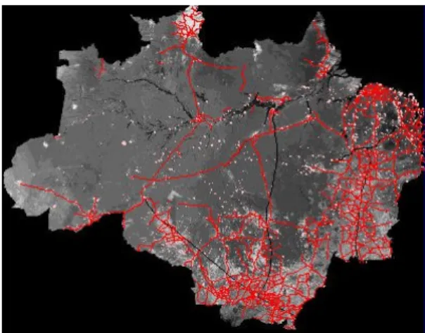
in Amazonia have to consider that transportation networks (rivers and roads) play a decisive role in governing human settlement patterns. As an illustration, Figure 1 shows the urban settlements in Amazonia, shown as white areas, and the road network in red lines. A realistic model for land use changes in the region has to take into account that the roads establish preferential directions for human occupation and land use changes, which would be impossible to be captured in isotropic neighborhoods prevalent in most spatial modeling techniques. The neighborhood definitions in any spatial model that aims at understanding the processes in an area such as Amazonia need to be based on flexible definitions of proximity that are able to capture action-at-a-distance.
Figure 1 – Human settlements (white dots) and roads (red) in Amazonia
To accommodate the concepts on absolute and relative space on a single construct, Couclelis [1]proposes the notion of proximal space, which aims to combine the concepts of absolute space
Couclelis [6]uses the metarelational map to extend traditional map algebra operations to operate over the proximal space, and thus captures spatial relations that act at a distance. The idea of relational map has been adapted by O’Sullivan [7]who proposes a graph-cellular automaton model (or graph-CA for short) for the representation of proximal space. A graph-CA extends the basic CA model by using a directed graph G. Each cell ciof
the CA is associated to a vertex vi of G and each
edge of the graph represents a relationship between two cells ci and cj. Applications of graph-CAs are
presented in O'Sullivan. [8]
This paper proposes a new model for the expression of the relations on the proximal space, using a generalized proximity matrix (or GPM for short). The GPM is an extension of the spatial weights matrix used in many spatial analysis methods (see, for example) [9], where the spatial weights are computed taking into account both
absolute space relations such as Euclidean distance or adjacency and relative space relations such as topological connection on a network. The GPM is particularly useful for the computation of spatial relations in proximal space, since it inherits well-established formalisms and techniques such as spatial autocorrelation indicators and spatial regression models, which have been defined using spatial weights matrices. We also show that the
graph-CA model can be expressed using the GPM model when a CA uses the GPM to express its neighborhood relations. We argue that the GPM is also a generalization of the metarelational map of Takeyama and Couclelis [6].
The paper is organized as follows. Section 2 gives the basic definitions associated to the GPM.
D1?…?Dn ? V1?…? Vn is the attribute function
that describes its properties.
We define a graph G over the same connected subset S ? ?2 as the set of spatial objects O and over a set of attribute domainsDn+1,..., Dn+k, each
associated to a value set Vn+i. The graph G is
composed of a set of nodes N and a set of arcs A.
Each node ni? N is defined by a tuple ni = [li, ?]
where the point li ? S is its location and ?i:
Dn+1?…?Dn ? Vn+1?…? Vn+k is its attribute
function. Each arc aij ? A represents a
relationship between two nodes ni and nj. An arc
is defined as aij = [ni, nj, L, ?], where L={p1,
…, pn}is a line describing its geometry (pi? S),
where p1 = ni.li and pn = nj.li, and whose
properties are described by its attribute function ?i:
Dn+1?…?Dn? V1?…? Vn.
Our definition of S includes objects with different types of geometric representation: (a) objects whose boundaries are closed polygons; (b) cellular automata and continuous fields organized as sets of cells, in which case the boundaries of each object are defined by the edges of each cell; (c) objects associated to point locations in two -dimensional space. Our definition of G includes different types of networks, including physical links (roads and rivers) and logical links (airline routes). This model of proximal space requires different representations of absolute and relative space using the sets S and G, since we consider that configuration of the relative space cannot be derived satisfactorily from the boundaries of spatial objects alone. Since the generalized proximity matrix is derived from a spatial weights matrix, it is useful to describe the usual techniques of derivation of the latter. Given two objects oi and ojfrom O,
moving local average for that attribute at each object is obtained by a weighted mean of all values of this attribute for all neighbors (as defined by the spatial weights matrix):
?
?
? ??
n j ij j n j ij iw
z
w
1 1ˆ
?
(4)In the above equation
?
ˆ
iis the local mean, wijis the element of the weights matrix that relates objects oi and oj, and zj is the value of the
attribute for the object oj. To allow spatial weights to be defined in proximal space, we define a generalized proxiity matrix (or GPM for short) as a spatial weights matrix created using generic strategies for the definition of spatial proximity, including not only the adjacency and distance relationships (which are defined in absolute space) but also relationships defined in relative space, such as connection through networks. The GPM aims to quantify the strength of non-local relationships between objects, and to incorporate the notion of proximal space in a weights matrix. Our concept of networks includes roads, rivers, airline routes, and telecommunication links.
3
Building Generalized Proximity
Matrices
As a general rule, each element wij of the
GPM is computed considering two types of proximity measures: one associated to absolute space relations and a second one associated to relative space relations. We denote by prox_abs
wij = ? *prox_abs (oi, oj)+ ? *
prox_rel(oi, oj) (6)
Prior to the definition of the prox_rel functions, we must first distinguish between two types of networks: (a) Networks in which the entrances and exits are restricted to its nodes, i.e., objects can be connected only at network nodes. Examples are railroads, telecommunication networks, banking networks, and productive chains. We denote these by closed networks; (b) networks in which any location can be used as entrance or exit point, i.e., objects can be connected at any node or arc coordinate. Examples are transportation networks such as roads and rivers. We denote these by open networks . For open networks, it is necessary to make use of the actual line coordinates that correspond to each arc in order to be able to compute the closest entrance/exit points from any arbitrary position.
The distinction between open and closed networks is application-dependent, but remains a valid one since the construction of the GPMs depends on the type of the network (open or closed) as explained below.
3.1
Proximity Measures in Open
Networks
In the case of open networks, a spatial object can be connected to the network at any point of any of the arc, and not only at the nodes. The proposed criterion for GPM construction considers two basic parameters: (a) the maximum distance from an object to the network; (b) the maximum value of the shortest path between the two connection points
measure. These measures use the following definitions: (a) All functions are defined in ?2, and a point x ? ?2 denotes a two -dimensional position in Cartesian coordinates; (b) Let O denote the set of spatial objects, and a graph G = (N, A) be composed of a set N of nodes and a set of arcs A; (c) Let cent: O? ?2 denote the function that calculates the centroid of a spatial object oi; (d)
Let dist: ?2 × ?2 ? ? the function that calculates the distance of two points x and y; (e) Let clspt: ?2 ×G? ?2 be the function, that given a location in ?2, determines the closest entry point in the graph; (f) Let shpath: ?2 ×?2 × G? ? be the function that calculates the shortest path between two locations on a graph.
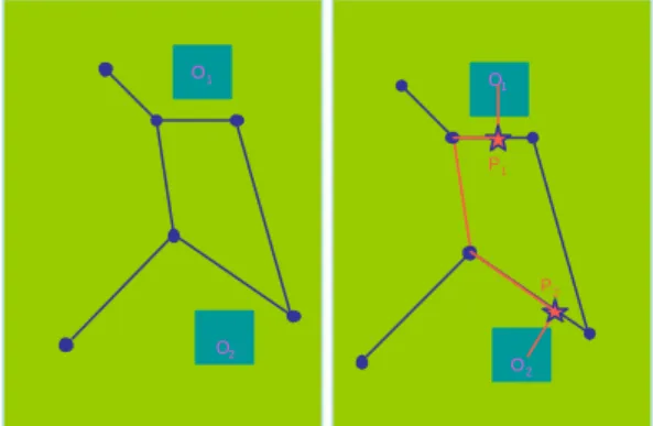
Given the above definitions, we can compute prox_rel, as illustrated in Figure 3. Given a pair of objects oi and oj in O and a graph G, the closest
locations in G to oi and oj are computed
(respectively pi and pj), and the shortest path
between pi and pj is calculated. The objects are
considered to be connected if: (a) the distance from their centroids to the network is smaller than a specified threshold (dmax); (b) the shortest path
between pi and pj in the graph is smaller than a
specified value (pmax). Two types of measurements
are possible, as follows:
?? Indicator function: prox_rel (oi,oj, G)
= 1 iff: ? pt ? G | dist (cent(oi), pt) < dmax AND (6) ? pt ? G | dist (cent(oj), pt) < dmax AND (7) If pt1 = clspt(cent(oi),G)and pt2 =
O1 O2 O1 O2 P2 P1
Figure 3. Schematic representation of algorithm for proximity measures in open networks.
3.2
Proximity Measures in Closed
Networks
In closed networks, the only entrance points are the nodes. In a similar way as in the case of open networks, two parameters are considered to identify connectivity between two spatial objects: the maximum distance from each object to the closest node and a maximum limit to the shortest path between the two nodes chosen as connection points, as illustrated in Figure 4. Given these parameters, the prox_rel function can be defined in a similar way as equations (6)-(8).
(b) proximity in relative space (open network connections). Forest Deforested No data Non -forest vegetation Water Roads 100 km Transamazônica Cuiabá-Santarém
São Felix do Xingu
Figure 5. Study Area in the Brazilian Amazonia, Pará State.
The study area is crossed by two non-paved main roads, Transamazônica and Cuiabá-Santarém. The human occupation in the
Transamazônica area dates mostly from the seventies ; one can notice the “espinha de peixe” (fish spine) spatial pattern, caused by the lotting schema adopted by state planners in that area. The Cuiabá-Santarém region is a new frontier area, where the forest has been less disturbed, which has received a large recent influx of new settlers coming mainly from the south. In the southeast of the study area, there is a more consolidated agricultural region named São Felix do Xingu, which is also served by a non-paved road. The huge undisturbed forest area in the middle of the study area contains several conservation units and indigenous areas, but it is also being threatened by new settlers coming from the São Felix do Xingu region.
(10)
In the above formula, the weights wij are
given by the GPM and n is the number of neighbors . The closer the values of an object’s attribute are those of its neighbours, the higher the index. Values around zero mean no correlation; higher positive values mean stronger positive correlation, and lower negative values mean stronger negative correlation. We also computed the statistical significance of the Local Moran Index, using 99 random permutations of the attribute values. Our goal was to analyze the behavior of such index given alternative neighborhood structures. We expected an increase in the indices when using the open network criterion (emphasis in relative space relations), especially for non-consolidated frontier areas, given that the deforestation process is known to spread from the road network. The results obtained confirm this hypothesis . For the cells connected to the network, the indices were, in average, approximately than 30% higher when using GPMs that take into account the relative space relations (open network criterion). We have selected five representative cells for discussion, shown in Figure 6 below. Forest Deforested No data Non-forest vegetation Cells examples Deforestation map: More consolidated Less consolidated C D A
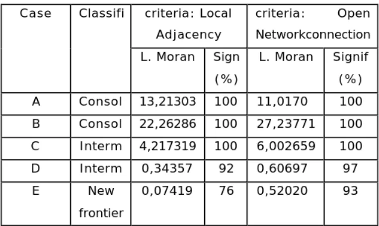
Table 1 – Local Moran index comparison for selected cells. criteria: Local Adjacency criteria: Open Networkconnection Case Classifi L. Moran Sign (%) L. Moran Signif (%) A Consol 13,21303 100 11,0170 100 B Consol 22,26286 100 27,23771 100 C Interm 4,217319 100 6,002659 100 D Interm 0,34357 92 0,60697 97 E New frontier 0,07419 76 0,52020 93
As mentioned before, the results confirm, in general, our hypothesis . In consolidated areas, network effects are less important due to the fact that the local adjacency neighborhood is able to capture the nature of the territorial dynamics. However, going to new frontier areas, the results obtained by the network connection are significantly higher than the ones obtained by the local adjacency neighborhood relations. We intend to continue to study the implications of alternative neighborhood structure s in spatial analysis techniques, specially aiming at understanding and modeling the land use and land cover change process in the Amazon.
5
GPMs as a Support for
Geo-Algebra and Graph-CA
In this section, we consider the relation of the GPM to geo-algebra [1]and graph-CA, [7] which are techniques that have been proposed to express relations in proximal space. The formalism for
geo-I
w z z
z
n
i ij i j j j j n?
? ??
?
1 2 1by a location l and a value v associated to each location. Then it follows that S is equivalent to M:L? V, as defined before; (b) Let ? be an operation over a set of numerical values, as above; (c) Let W be a generalized proximity matrix where each wij is either 1 or 0, indicating the presence or absence of a relation between the locations li and lj. It follows that each line i of W contains the
same information as the relational map Ri; (d) For
each location li, let the set of values Vi be
computed as the product of the weig hts wij and the
values M(lj), ? lj? L. In this case, this set of
values is the same as the one produced by applying the relational map Rl to the map M; (e) The
geo-algebra operations can be defined by the application of the operation ? to all sets Vi in the map:
M(i)new = ?({Vi}), where Vi =
{(wij * M(lj))},? lj? L. (11)
Therefore, the geo-algebra of Takeyama and Couclelis [6] can be obtained by a suitable choice of a GPM and by defining all map algebra functions to be calculated using the GPM. In a similar fashion, the GPM can provide support for the graph-CA technique[7]. Recall that a CA can be defined by a tuple (X,S,N,f) in which:
(i) X?Z2 is the celular space;
(ii) S is the finite set of possible states; (iii) N(x) = {x1,...,xk}, is set of
cells that are in the neighborhood of a cell x ? X.
(iv) f:Sk? S is the transition function defined as S(x,t)=f(S(x1,t),...,
S(x t)), ? x ? N(x), where
generic way of expressing spatial relations in proximal space.
6
Open Source Software for GPM Usage
We have implemented the concepts described in this paper using the Terralib environment, an open source GIS library available at http://www.terralib.org. [12] TerraLib provides functionality for handling the different types of geographical data and facilities for data conversion, graphical output, and spatial database management using a spatially-enabled object-relational DBMS (such as ORACLE and PostgreSQL). We have extended TerraLib by implementing a set of C++ classes to support the creation and manipulation of generalized proximity matrices. The GPM is then used in lieu of spatial weights matrices for all spatial analysis applications and cellular automata simulations.7
Conclusions
In today’s globalized world, where flows of resources and information are becoming increasingly important, spatial information systems need to incorporate flexible definitions of space. The generalized proximity matrix (GPM), a concept introduced in this paper, is able to combine neighbourhood criteria based both absolute and relative space definitions this allowing to combine local actions with action-at-a-distance. In this paper, we indicate how the matrix can be calculated, considering different types of network configurations. We have also presented a case study where the GPM has been shown to capture spatial relationships that we not detected by considering only local adjacency, by including network
References
1. Couclelis, H., From Cellular Automata to Urban Models: New Principles for Model Development and Implementation.
Environment and Planning B: Planning and Design, 1997. 24: p. 165-174.
2. Schuurman, N., Critical GIS: Theorizing an emerging science. Cartographica, 1999. 36(4): p. 1-108.
3. Soja, E.W., Postmodern Geographies: The Reassertion of Space in Critical Social Theory. 1989, London: Verso.
4. Harvey, D., The Condition of Postmodernity. 1989, London: Basil Blackwell.
5. Castells, M., A Sociedade em Rede. 1999, São Paulo: Paz e Terra.
6. Takeyama, M. and H. Couclelis, Map Dynamics: Integrating Cellular Automata and GIS through Geo-Algebra. International Journal of Geographical Information Systems, 1997. 11(1): p. 73-91.
7. O'Sullivan, D., Graph-cellular automata: a generalised discrete urban and regional model. Environment and Planning B: Planning and Design, 2001. 28: p. 687-705.
8. O'Sullivan, D., Exploring spatial process dynamics using irregular graph-based cellular automaton models. Geographical Analysis, 2001. 33: p. 1-18.
9. Bailey, T. and A. Gattrel, Spatial Data Analysis by Example. 1995, London: Longman.
10. Anselin, L., Interactive techniques and Exploratory Spatial Data Analysis, in
Geographical Information Systems: principles, techniques, management and applications, P. Longley, et al., Editors. 1999, Geoinformation International: Cambridge.
11. Anselin, L., Local indicators of spatial association - LISA. Geographical Analysis, 1995. 27: p. 91-115.
12. Câmara, G., et al. TerraLib: Technology in Support of GIS Innovation. in II Workshop Brasileiro de Geoinformática, GeoInfo2000. 2000. São Paulo.