On Some Ridge Regression Estimators for Logistic Regression Models

(1)

Florida International University

FIU Digital Commons

FIU Electronic Theses and Dissertations

University Graduate School

3-28-2018

On Some Ridge Regression Estimators for Logistic

Regression Models

Ulyana P. Williams

Florida International University, [email protected]

DOI:

10.25148/etd.FIDC006547

Follow this and additional works at:

https://digitalcommons.fiu.edu/etd

Part of the

Applied Statistics Commons

,

Other Statistics and Probability Commons

, and the

Statistical Methodology Commons

This work is brought to you for free and open access by the University Graduate School at FIU Digital Commons. It has been accepted for inclusion in FIU Electronic Theses and Dissertations by an authorized administrator of FIU Digital Commons. For more information, please [email protected].

Recommended Citation

Williams, Ulyana P., "On Some Ridge Regression Estimators for Logistic Regression Models" (2018).FIU Electronic Theses and

Dissertations. 3667.

(2)

FLORIDA INTERNATIONAL UNIVERSITY

Miami, Florida

ON SOME RIDGE REGRESSION ESTIMATORS FOR LOGISTIC REGRESSION MODELS

A thesis submitted in partial fulfillment

of the requirements for the degree of

MASTER OF SCIENCE

in

STATISTICS

by

Ulyana Williams

2018

(3)

ii

To: Dean Michael R. Heithaus

College of Arts, Sciences and Education

This dissertation, written by Ulyana Williams, and entitled

On Some Ridge Regression

Estimators for Logistic Regression Models

, having been approved in respect to style and

intellectual content, is referred to you for judgment.

We have read this dissertation and recommend that it be approved.

_______________________________________

Jie Mi

_______________________________________

Florence George

_______________________________________

B.M. Golam Kibria, Major Professor

Date of Defense: March 28, 2018

The dissertation of Ulyana Williams is approved.

_______________________________________

Dean Michael R. Heithaus

College of Arts, Sciences and Education

_______________________________________

Andrés G. Gil

Vice President for Research and Economic Development

and Dean of the University Graduate School

(4)

iii

ABSTRACT OF THE THESIS

ON SOME RIDGE REGRESSION ESTIMATORS FOR LOGISTIC REGRESSION MODELS

by

Ulyana Williams

Florida International University, 2018

Miami, Florida

Professor B. M. Golam Kibria, Major Professor

The purpose of this research is to investigate the performance of some ridge regression

estimators for the logistic regression model in the presence of moderate to high correlation among

the explanatory variables. As a performance criterion, we use the mean square error (MSE), the

mean absolute percentage error (MAPE), the magnitude of bias, and the percentage of times the

ridge regression estimator produces a higher MSE than the maximum likelihood estimator.

A Monto Carlo simulation study has been executed to compare the performance of the

ridge regression estimators under different experimental conditions. The degree of correlation,

sample size, number of independent variables, and log odds ratio has been varied in the design of

experiment.

Simulation results show that under certain conditions, the ridge regression estimators

outperform the maximum likelihood estimator. Moreover, an empirical data analysis supports the

main findings of this study.

This thesis proposed and recommended some good ridge regression estimators of the

logistic regression model for the practitioners in the field of health, physical and social sciences.

(5)

iv

ACKNOWLEDGMENTS

I would like to express my sincere gratitude to my advisor Prof. B. M. Golam Kibria for

the continuous support of my M.S study and related research. Also, I have to thank Prof. Kristofer

Mansson for assistance with simulation study. Besides my advisor, I would like to thank the rest

of my thesis committee: Prof. Jie Mi, Prof. George Florence for their contributions in the

completion of this thesis. Finally, I must express my very profound gratitude to my parents and to

my husband for providing me with support throughout my years of study.

(6)

v

TABLE OF CONTENTS

CHAPTER PAGE

I. INTRODUCTION ... 1

1.1 Literature Review...1

1.2 Research Purpose and Tasks...2

II.STATISTICAL METHODOLOGY...3

2.1 Logistic Regression Model...3

2.2 Estimation of the Ridge Parameter k...5

2.3 Criterions of a Good Estimator...10

III. SIMULATION STUDY... 11

3.1 Simulation Techniques...11

3.2 Result Discussion...12

3.3 Some Proposed New Estimators of k...17

IV. APPLICATION... 20

V. SUMMARY AND CORRESPONDING REMARKS...22

REFERENCES...24

(7)

vi

LIST OF FIGURES

FIGURE PAGE

1.

Performance of estimators as a function of sample size for p = 4, ρ =0.95, intercept = 0...

.12

2. Performance of estimators as a function of sample size for p = 4, ρ =0.95, intercept = 0...13

3. Performance of the estimators as a function of ρ when p = 4, n = 100 and intercept = 0...14

4. Performance of the selected estimators as a function of ρ when p = 4, n = 100, intercept = 0...14

5. Performance of the estimators as a function of ρ when p = 8, n = 100 and intercept = 0...15

6. Performance of the selected estimators as a function of ρ when p = 8, n = 100, intercept = 0...15

7. Performance of the estimators as a function of p with ρ = 0.95, n = 100 and intercept = 0...16

8. Figure 8. Performance of the estimators as a function of the intercept

when ρ = 0.95, n = 100 and p = 4...17

9. Performance of estimators as a function of sample size for p = 4, ρ =0.95, intercept = 0...18

10. Performance of estimators as a function of sample size for p = 4, ρ =0.95, intercept = -1...19

(8)

1

CHAPTER I

INTRODUCTION

1.1 Literature Review

In a multiple linear or non-linear regression model, one may deal with near- linear

dependency among the explanatory variables known as a multicollinearity. If two or more

explanatory variables are highly correlated with one another, methods such as the least squares

and maximum likelihood (ML) for estimating the regression parameters give a very poor

precision of the estimates. There is perfect multicollinearity if absolute value of the correlation

coefficient between two independent variables is equal to 1. We seldom have perfect

multicollinearity in practice. In general, if simple correlation coefficient between two regressors

is greater than 0.8 or 0.9 or variance inflation factor is greater than 3, the multicollinearity will

affect calculations regarding individual predictors by inflating the variance of the parameter

estimates (see Mansson, 2011).

One of the many remedies for solving the multicollinearity problem, is to use the ridge

regression method proposed by Hoerl and Kennard (1970). Their work is the most frequently

cited in the literature and generally regarded as the seminal paper on the subject. Many authors

have worked on developing estimates for ridge regression parameter for the mainly linear

regression models. To mention a few, Lawless and Wang (1976), Kibria (2003), Khalaf and

Shukur (2005), Alkhamisi, Grhadban and Shukur (2007), Gisela and Kibria (2009) and very

recently Kibria and Banik (2016) and Asar and Genc (2017) among others. However, few

researchers have been studying non-linear ridge regression model, such as the logistic ridge

regression model. Among them Schaefer et al. (1984), Hoerl et al. (1975), Mansson and Shukur

(2011) and very recently

Månsson

(2017) are notable. This thesis expands on that study by

evaluating more ridge estimators and proposing some new k estimators for the logistic ridge

regression model.

(9)

2

Logistic regression is a widely used method for categorical data. It is a type of regression

model where the response variable is a dichotomous variable and the independent variables are

continuous or categorical. The logistic regression widely employed in many fields, such as

epidemiological research, health science and social sciences. A very good example of this model

is to investigate the occurrence of a disease as related to different characteristics of patients, such

as, age, sex, food habit, calorie intake etc. The motivational example of this model is to predict the

recreational trip of the registered leisure boat owners in 23 counties of East Texas using the

following explanatory variables: facility's subjective quality ranking, respondent's taste for

water-skiing, travel cost to Lake Conroe, travel cost to Lake Somerville, travel cost to Lake. The Texas

example will be analyzed in Chapter 4.

1.2 Research Purpose and Tasks

The present thesis will propose different methods for estimating the ridge parameter,

k.

In

order to judge the performance of the estimators, we need to compare these estimators under

different performance criterion. The main objective of my research is to investigate the

performance of the popular ridge estimators for the logistic regression model in the presence of

moderate to high correlation among the explanatory variables employing the following criteria:

1. Mean squared error (MSE),

2. Mean absolute percentage error (MAPE),

3. Magnitude of bias,

4. Performance of ridge regression estimator compared to the ML estimator, in terms of the

percentage of times the ridge regression estimator produces a higher MSE than the ML estimator.

The organization of the thesis is as follows. We define different ridge regression estimators of

k

in Chapter 2. A Monte Carlo simulation study is conducted in Chapter 3. In Chapter 4, the

empirical application of the ridge logistic regression will be presented. Summary and concluding

remarks are given in Chapter 5.

(10)

3

CHAPTER II

STATISTICAL METHODOLOGY

2.1 Logistic Regression Model

Logistic regression is one of the most commonly used tools for applied statistics to explain

the relationship between dependent binary variable and discrete and/or continuous explanatory

variables. The jth value of the dependent variable

Y

of the regression model is Bernoulli random

with the following parameter

𝜋

j

(see Mansson (2011)):

𝜋

j

= P(y

j

= 1) =

exp⁡(𝐱𝒋𝛃)

1+⁡exp⁡(𝐱𝒋𝛃)

, j = 1, . . . , n (2.1)

where

𝐱

𝑗

is the j

th

row of n × (p + 1) data matrix

𝜲

and

β

is a (p + 1) × 1 vector of coefficients.

The most common method to estimate

β

is to apply ML method because this method does not

require any restrictions on the characteristics for independent variables.

The joint PMF of y

j

’s is given by

L

(

β|

𝜲

) =

∏

𝑛𝑗=1

{𝜋

_𝑗𝑦𝑗

⁡(1 − ⁡ 𝜋

𝑗

)

1−⁡𝑦𝑗

}

(2.2)

and the log likelihood function by

log (

L

(

β|

𝜲

)) =

∑

𝑗=1𝑛

𝑦

𝑗

log(𝜋

𝑗

) + ⁡ ∑

𝑛𝑗=1

(1 − ⁡ 𝑦

𝑗

) log(1 − ⁡ 𝜋

𝑗

)

. (2.3)

To find the MLE of

β

we need to take the first derivative of the above equation and solve the

likelihood equation

𝜕⁡log⁡(𝐿(𝛃|⁡𝚾))

𝜕𝛃

=

∑

x

𝑗

𝑛

𝑗=1

(𝑦

𝑗

− ⁡ 𝜋

𝑗

)

= 0 (2.4)

which is nonlinear in

β

. The most common method of obtaining the MLE is to apply the iteratively

weighted least squares algorithm as follows (see Mansson(2011)):

𝛽̂

𝑀𝐿

=

(𝛸

′

𝑊

̂ ⁡𝛸⁡)

−1

𝛸

′

𝑊

̂ 𝑧̂

, (2.5)

where

𝑊

̂

= diag (

𝜋̂

𝑗

(1 -

𝜋̂

𝑗

)) and

𝑧̂

𝑗

= log(

𝜋̂

𝑗

) +

𝑦𝑗−⁡𝜋̂𝑗

𝜋

̂_𝑗(1⁡−⁡𝜋̂_𝑗)⁡

is the

j

th

(11)

4

The asymptotic variance-covariance matrix of the ML estimator is obtained by differentiating

log-likelihood function second time with respect to each element of

β

, denoted by

𝛃

′

(see

Mansson(2011)):

𝜕 2_{⁡log⁡(𝐿(β|⁡Χ))} 𝜕β⁡𝜕β′

=

𝜕 𝜕β′

⁡∑

x

𝑗 𝑛 𝑗=1

(𝑦

𝑗

− ⁡ 𝜋

𝑗

)

= -

𝜕 𝜕β′

⁡∑

x

𝑗 𝑛 𝑗=1

𝜋

𝑗

= -

⁡∑

𝑛𝑗=1

x

𝑗

⁡𝜋

𝑗

(1 − ⁡ 𝜋

𝑗

)⁡x

𝑗′

⁡

=

(𝛸

′

𝑊

̂ ⁡𝛸⁡)

−1

.

(2.6)

One of the disadvantages of using ML method is that the ML estimator can be affected by the

presence of collinearity. Because of collinearity in X matrix, the elements of

(𝛸

′

𝑊

̂ ⁡𝛸⁡)

−1

will be

large and consequently the variance of ML estimator become inflated. To combat the problem of

multicollinearity, the ridge logistic estimator has been proposed (see Schaefer, 1986). It is defined

as

𝛽̂

𝑅

(𝑘)

=

(𝛸

′

𝑊

̂ ⁡𝛸 + 𝑘𝐼⁡)

−1

𝛸

′

𝑊

̂ ⁡𝛸𝛽̂

𝑀𝐿

=

𝑉𝛽̂

𝑀𝐿

,

k

> 0 (2.7)

where

𝑉 = (𝛸

′

𝑊

̂ ⁡𝛸 + 𝑘𝐼⁡)

−1

𝛸

′

𝑊

̂ ⁡𝛸

. The asymptotic mean square error (MSE) of the ridge

estimator is obtain as follows (see Mansson (2011)):

MSE (

𝛽̂

𝑅

(k))

=

E

[

(𝑉𝛽̂𝑀𝐿

− ⁡𝛽)

′

(

𝑉𝛽̂𝑀𝐿

– β

)]

=

E

((𝛽̂

𝑀𝐿

− ⁡𝛽)

′

𝑉′𝑉

(

𝛽̂

𝑀𝐿

– β

)) +

E

(

𝛽

′

(𝑉 − 𝐼)

′

(𝑉 − 𝐼)

β

)

+ 2*

E

(

(𝛽̂

𝑀𝐿

− ⁡𝛽)′𝑉′(𝑉 − ⁡𝐼)𝛽)

).

It is known that for large

n

,

(𝛽̂

𝑀𝐿

− ⁡𝛽

) ~ N (0,

(𝛸

′

𝑊

̂ ⁡𝛸⁡)

−1

) (see Lee (1988)).

Therefore,

E

(

(𝛽̂

𝑀𝐿

− ⁡𝛽)′𝑉′(𝑉 − ⁡𝐼)𝛽)

) = 0.

Then the MSE becomes as follows:

MSE (

𝛽̂

𝑅

(k))

=

E

((𝛽̂

𝑀𝐿

− ⁡𝛽)

′

𝑉′𝑉

(

𝛽̂

𝑀𝐿

– β

)) +

E

(

𝛽

′

(𝑉 − 𝐼)

′

(𝑉 − 𝐼)

β

)

E

((𝛽̂

𝑀𝐿

− ⁡𝛽)

′

𝑉′𝑉

(

𝛽̂

𝑀𝐿

– β

)) =

tr

(

E

(𝑉(𝛽̂

𝑀𝐿

⁡– ⁡𝛽)

(

𝛽̂

𝑀𝐿

– β

)

⁡′𝑉

′

)) =

𝑡𝑟(𝑉𝐶𝑜𝑣(𝛽̂

𝑀𝐿

)𝑉

′

) =

⁡𝑡𝑟(𝑉(𝛸

′

𝑊

̂ ⁡𝛸⁡)

−1

𝑉′)

=

𝑡𝑟((𝛸

′

𝑊

̂ ⁡𝛸 + 𝑘𝐼⁡)

−2

𝛸

′

𝑊

̂ ⁡𝛸)

.

(12)

5

=

𝛽

′

(𝑘

2

(𝛸

′

𝑊

̂ ⁡𝛸 + 𝑘𝐼⁡)

−2

)

𝛽

Let

C

=

𝜲

′

𝑾

̂

𝜲

and

Ʌ =

diag

(

𝜆

1

, ....

𝜆

𝑝

)

Suppose there exists an

orthogonal matrix

P

, such that

𝑷′𝑪𝑷

=

Ʌ

, then

𝑡𝑟((𝛸

′

𝑊

̂ ⁡𝛸 + 𝑘𝐼⁡)

−2

𝛸

′

𝑊

̂ ⁡𝛸)

=

𝑡𝑟(𝑃𝑃′(𝛸

′

𝑊

̂ ⁡𝛸 + 𝑘𝐼⁡)

−1

𝑃𝑃

′

(𝛸

′

𝑊

̂ ⁡𝛸 + 𝑘𝐼⁡)

−1

𝑃𝑃′𝛸

′

𝑊

̂ ⁡𝛸)

=

𝑡𝑟 (𝑃

′

(𝛸

′

𝑊

̂ ⁡𝛸 + 𝑘𝐼⁡)

−1

𝑃𝑃

′

(𝛸

′

𝑊

̂ ⁡𝛸 + 𝑘𝐼⁡)

−1

𝑃𝑃

′

𝛸

′

𝑊

̂ ⁡𝛸𝑃)⁡

=

= 𝑡𝑟 ((𝑃

′

𝛸

′

𝑊

̂ ⁡𝛸𝑃 + 𝑘𝐼⁡)

−1

(𝑃

′

𝛸

′

𝑊

̂ ⁡𝛸𝑃 + 𝑘𝐼⁡)

−1

𝑃′𝛸

′

𝑊

̂ ⁡𝛸𝑃)

=

𝑡𝑟((Ʌ + 𝑘𝐼⁡)

−1

(Ʌ + 𝑘𝐼⁡)

−1

Ʌ

)=

=

∑

𝜆𝑖 (𝜆𝑖+𝑘)2 𝑝 𝑖=1

(2.8)

k

2

𝛽

′

(𝛸

′

𝑊

̂ ⁡𝛸 + 𝑘𝐼)

−2

𝛽

=

k

2

(𝑃𝛽)

′

(𝑃

′

𝛸

′

𝑊

̂ ⁡𝛸𝑃 + 𝑘𝑃𝑃

′

)

−2

(𝑃𝛽) =⁡

𝑘

2

⁡∑

𝛼𝑖2 (𝜆𝑖⁡+𝑘)2 𝑝 𝑖=1

(2.9)

So, MSE (

𝛽̂

𝑅

(k))⁡

=

Var

(

𝛽̂

𝑅

)

+ (Bias (

𝛽̂

𝑅

))

2

=

∑

𝜆𝑖 (𝜆_𝑖+𝑘)2 𝑝 𝑖=1

+

𝑘

2

⁡∑

𝛼_𝑖2 (𝜆_𝑖⁡+𝑘)2 𝑝 𝑖=1

,

(2.10)

where

𝜆

𝑖

is the i

th

eigenvalue of the

𝚾

′

𝐖

̂ ⁡𝚾

matrix and

α

=

Pβ

(see Mansson (2011)).

The first term in Eq. (2.10) is a continuous, monotonically decreasing function of

k

, and the

second term is a continuous, monotonically increasing function of

k.

For large value of

k,

the

variance vanishes and the bias dominates the MSE. The main goal of logistic ridge regression

method is to find an appropriate

k

such that the decrease in variance of the ridge regression

estimator exceeds the increase in its bias.

2.2 Estimation of the Ridge Parameter k

.

The first method of choosing the biasing or ridge parameter

k

was proposed by Hoerl and

Kennard (1970) for linear regression model. It states that there always exists a k > 0 such that MSE

(

𝛽̂

𝑅

(k))

< MSE (

𝛽̂𝑀𝐿)

. Schaefer (1984) followed the same principal to find the ridge parameter for

(13)

6

logistic regression. To show that we minimize the mean square error of ridge estimator, the first

derivative of Eq. (2.10) with respect to

k

is

𝜕⁡MSE⁡(𝛽̂𝑅) 𝜕𝑘

= -2

∑

𝜆_𝑖 (𝜆_𝑖+𝑘)3 𝑝 𝑖=1

+ 2

𝑘⁡ ∑

𝜆_𝑖𝛼_𝑖2 (𝜆_𝑖⁡+𝑘)3 𝑝 𝑖=1

. (2.11)

Since

𝜆𝑖

> 0, the first derivatives of the first and second terms are always non-positive and

non-negative, respectively. We note that when

k

is equal to zero

𝛽̂

𝑅

(𝑘)

=

𝛽̂

𝑀𝐿

with equal variance

∑

1

𝜆_𝑖 𝑝

𝑖=1

and zero bias.

Moreover, the optimal value of any individual parameter

k

i

can be found by setting Eq.

(2.11) to zero and solve for

k

. Then it can be shown that

𝑘

𝑖

=

1

𝛼_𝑖2

(2.12)

The optimal value of

k

i

fully depends on the unknown

𝛼

𝑖

, which can be estimated from the

data. Schaeffer et al. (1984) suggested to replace

𝛼

𝑖

by its estimator

𝛼̂

𝑖

.That means, the optimum

value if

k

is obtained as follows:

𝑘̂

𝐻

=

1

𝛼̂_𝑖2

(2.13)

Schaefer (1984) showed that the optimal value of

k

for ridge logistic regression model as

follows:

𝑘̂

𝐻1

= ⁡

1

𝛼̂_𝑚𝑎𝑥2

(2.14)

Hoerl

et al.

(1975) suggested a different estimator of

k

taking the harmonic mean of the

ridge parameter

𝑘̂𝑖

. The estimator is given as:

𝑘̂

𝐻2

= ⁡

𝑝 ∑𝑝 𝛼̂_𝑖2

𝑖=1

=

_𝛼_̂𝑝_′_𝛼_̂

(2.15)

Lawless and Wang (1976) proposed the following ridge estimator for

k

:

𝑘̂

𝐿𝑖

=

1

𝛼̂_𝑖2𝜆_𝑖

(2.16)

and represent as a single value by taking harmonic mean of

𝑘̂

𝐿𝑖

:

(14)

7

𝑘̂

𝐿

= ⁡⁡

𝑝 ∑𝑝_𝑖=1𝛼̂_𝑖2𝜆_𝑖

=

𝑝 𝛼̂′⁡_𝑋′_𝑋⁡𝛼_̂

(2.17)

Hocking et al. (1976) suggested the following estimator:

𝑘̂

𝐻𝐺

= ⁡

∑𝑝 (𝜆_𝑖𝛼̂_𝑖)2 𝑖=1 (∑ 𝜆𝑖𝛼̂𝑖2) 𝑝 𝑖=1 2

(2.18)

Batah et.al (2008) suggested the following:

𝑘̂𝐵𝐻

= ⁡⁡

𝑝 ∑ [ 𝛼̂_𝑖2 (𝛼̂𝑖4𝜆𝑖 2 4 + 6𝛼_̂𝑖2𝜆_𝑖 1 ) 1/2 −⁡𝛼̂𝑖2𝜆₂𝑖⁡ ⁡ ] 𝑝 𝑖=1

(2.19)

Noruma (1988) proposed the following estimator:

𝑘̂

𝑁𝑅

= ⁡

𝑝 ∑ [ 𝛼̂𝑖 2 ⁡1+⁡(1+𝜆𝑖(𝛼̂𝑖2)1/2⁡) ] 𝑝 𝑖=1

.

(2.20)

Kibria (2003) proposed new estimators for

k

by taking the geometric mean, arithmetic mean

and median (p ≥ 3) of the ridge estimator of

𝑘̂

𝑖

. These estimators are represented respectively as

follows:

𝑘̂

𝐾1

= ⁡

1 (∏𝑝_𝑖=1𝛼̂_𝑖2)1/𝑝

(2.21)

𝑘̂

𝐾2

= ⁡

1 𝑝

∑

1 𝛼 ̂_𝑖2 𝑝 𝑖=1

(2.22)

𝑘̂𝐾3

= 𝑚𝑒𝑑 (

_𝛼_̂1 𝑖2

).

(2.23)

Furthermore, Muniz et al (2009, 2012) proposed some estimators of

k

in the following form:

The square root of the geometric mean of

𝑘̂

𝑖

𝑘̂

𝐾4

=

∏

(√

1 𝛼̂_𝑖2

)

1/𝑝 𝑝 𝑖=1

(2.24)

The reciprocal of the square root of the geometric mean of

𝑘̂

𝑖

𝑘̂

𝐾5

=

∏

(

1 √_𝛼_̂1 𝑖 2

)

1/𝑝 𝑝 𝑖=1

(2.25)

(15)

8

The median of the square root of

𝑘̂

𝑖

𝑘̂

𝐾6

=

𝑚𝑒𝑑(√

1 𝛼

̂_𝑖2

)

(2.26)

The maximum of the reciprocal of the square root of

𝑘̂

𝑖

𝑘̂

𝐾7

=

𝑚𝑎𝑥(

1 √_𝛼_̂1 𝑖 2)

)

(2.27)

The median of the reciprocal of the square root of

𝑘̂

𝑖

𝑘̂𝐾8

=

𝑚𝑒𝑑(

1

√_𝛼_̂1

𝑖 2)

)

(2.28)

The maximum of the square root of

𝑘̂𝑖

𝑘̂

𝐾9

=

𝑚𝑎𝑥(√

1 𝛼

̂_𝑖2

)

(2.29)

Doruge (2013) proposed a new estimator for

k

by multiplying the denominator with

𝜆

𝑚𝑎𝑥

/2:

𝑘̂𝐷𝑖

=

2

𝜆_{𝑚𝑎𝑥⁡}𝛼̂_𝑖2

(2.30)

Lukman et al (2017) proposed the following estimators:

𝑘̂

𝐿1

= 𝑚𝑎𝑥(

2 𝜆_{𝑚𝑎𝑥⁡}𝛼̂_𝑖2

)

(2.31)

𝑘̂

𝐿2

= 𝑚𝑎𝑥(1/

2 𝜆𝑚𝑎𝑥⁡𝛼̂𝑖2

)

(2.32)

Following Kibria (2003), the modification on the Doruge’s estimator also have been

performed:

𝑘̂

𝐷1

= ⁡

2𝑝 𝜆𝑚𝑎𝑥⁡∑ 𝛼̂𝑖2 𝑝 𝑖=1

(2.33)

𝑘̂

𝐷2

= 𝑚𝑒𝑑(

2 𝜆𝑚𝑎𝑥⁡𝛼̂𝑖2

)

(2.34)

𝑘̂

𝐷3

= ⁡

2 𝜆𝑚𝑎𝑥⁡(∏ 𝛼̂𝑖2) 𝑝 𝑖=1 1/𝑝

(2.35)

𝑘̂

𝐷4

= ⁡

2 𝜆𝑚𝑎𝑥⁡𝑝

∑

1 𝛼̂_𝑖2 𝑝 𝑖=1

(2.36)

(16)

9

Khalaf and Shukur (2005) suggested a new estimator of

k

as modification of

𝑘̂

𝐻1

:

𝑘̂

𝐾𝑆

=

𝜆𝑚𝑎𝑥

(𝑛−𝑝)+𝜆𝑚𝑎𝑥𝛼̂𝑚𝑎𝑥2 ⁡

.

(2.35)

Kibria

et al.

(2012) and Alkhamisi (2006) proposed new estimators based on modifications

of

q

i

=

𝜆𝑚𝑎𝑥 (𝑛−𝑝)+𝜆𝑚𝑎𝑥𝛼̂𝑖2⁡

as follows:

𝑘̂

𝐾𝑆1

=

𝑚𝑎𝑥(√𝑞𝑖

)

(2.36)

𝑘̂

𝐾𝑆2

=

𝑚𝑎𝑥(

1 √𝑞𝑖

)

(2.37)

𝑘̂

𝐾𝑆3

=

𝑚𝑒𝑑(

1 √𝑞𝑖

)

(2.38)

𝑘̂

𝐾𝑆4

=

(∏

𝑝𝑖=1

√𝑞𝑖

)

1/𝑝

(2.39)

𝑘̂

𝐾𝑆5

=

(∏

1 √𝑞𝑖 𝑝 𝑖=1

)

1/𝑝

(2.40)

𝑘̂

𝐴𝑙1

=

𝑚𝑎𝑥(𝑞

𝑖

)

(2.41)

𝑘̂

𝐴𝑙2

= ⁡

1 𝑝

∑

𝑞

𝑖 𝑝 𝑖=1

(2.42)

Alkhamisi and Shukur (2007) suggested some new estimators of

k

as modification of

𝑘̂

𝐻1

:

𝑘̂

𝐴𝑆1

=

𝑘̂

𝐻1

+ ⁡

1

𝜆𝑚𝑎𝑥

(2.43)

and its functions as

𝑘̂

𝐴𝑆2

=

𝑚𝑎𝑥(

1 𝛼 ̂_𝑖2

+ ⁡

1 𝜆_𝑚𝑎𝑥

)

(2.44)

𝑘̂

𝐴𝑆3

=

𝑚𝑒𝑑(

1 𝛼̂_𝑖2

+ ⁡

1 𝜆_𝑚𝑎𝑥

)

(2.45)

𝑘̂

𝐴𝑆4

= ⁡

1 𝑝

∑

1 𝛼 ̂_𝑖2

+ ⁡

1 𝜆𝑚𝑎𝑥 𝑝 𝑖=1

( 3.46)

Furthermore, Alkhamisi and Shukur (2007) proposed new estimator based on Lawless and

Wang (1976):

𝑘̂

𝐴𝑆5

=

𝑘̂

𝐿

+ ⁡

1

(17)

10

Since, just a few estimators of

k

have been studied for the ridge logistic regression in

literature, all proposed estimators of

k

are under consideration.

2.3 Criterion of a Good Estimator

In the current study we employed different criteria to evaluate the performance of ridge

parameter,

k

. The main criterion is to investigate the performance of the estimators is the mean

square error (MSE). It defines as follows:

Average MSE =

∑ (𝛽̂−𝛽) ′ (𝛽̂ −𝛽) 2000 𝑟=1 2000

, at

r

th

step of the simulation (2.48)

In case of equal MSEs for any two estimators, we will prefer the estimator with smaller

bias. Therefore, the average bias has been calculated for each proposed estimator as follows

Average Bias =

∑ 𝑏𝑖𝑎𝑠(𝛽̂)

2000 𝑟=1

2000

, at

r

th

where

𝑏𝑖𝑎𝑠(𝛽̂)

= -

𝑘̂

Uβ , U =

(𝑋

′

𝑊

̂ 𝑋 + 𝑘̂𝐼)

−1

.

Another interesting criteria of performance of the estimators is the Mean Absolute Percent

Error (MAPE) which measures the size of the error in percentage terms. It defines as

Average MAPE =

∑ 𝑀𝐴𝑃𝐸(𝛽̂)

2000 𝑟=1

2000

, at

r

th

where

𝑀𝐴𝑃𝐸(𝛽̂)

=

1 𝑝

∑

|𝛽̂−𝛽| |𝛽| 𝑝 𝑖=1

.

In addition, the proportion of replication (out of 2000) for which ML estimator had a

smaller MSE than the proposed ridge regression estimator has been presented.

(18)

11

CHAPTER III

SIMULATION STUDY

Since a theoretical comparison among the estimators is not possible, a Monte Carlo

simulation study has been conducted to compare the performance of the estimators in Chapter

Three. We use R-3.2.2 software to complete the simulation study.

3.1 Simulation Techniques

The main factor in the design of the experiment is the degree of correlation between the

regressors. To vary the strength of the correlation, following Kibria (2003) we generate the datasets

by using

𝑥

𝑗𝑖

=

(1 − ⁡ 𝜌

2

)

1/2

𝑧

𝑗𝑖

+

𝜌𝑧𝑗𝑝

i

= 1, 2, . . . ,

p j

= 1, 2, . . . ,

n

(3.1)

where

𝑧

𝑗𝑖

are independent standard normal pseudo-random numbers and

ρ

is specified such that the

correlation between two explanatory variables is given by

𝜌

2

. The main restriction in simulation

study without loss of generality is that the parameter values of

β

are equal and chosen so that

∑

𝑝_𝑖=1

𝛽

_𝑖2

= 1 (see Kibria 2003). For given X matrix and

β

, the n observations for dependent variable

y

was obtained from Be(

𝜋

j

) distribution, where

𝜋

j

= P(y

j

= 1) =

exp⁡(𝐱𝒋𝛃)

1+⁡exp⁡(𝐱𝒋𝛃)

, j = 1, . . . , n (3.2)

In the simulation technique, four different values of

ρ

as 0.75, 0.85, 0.95, 0.99 are used. To

investigate the effect of the sample sizes on the performance of the estimator, we will set sample

size

n

as 70, 100, 200. Also, we consider

p

= 4 and

p

= 8 explanatory variables. Another

consideration is taken to the value of the intercept since it represents the average value of the log

odds ratio. In the simulation study we set the value of intercept be -1 ,0, and 1.

For given values

n, ρ

,

p

, and intercept, the set of explanatory variables was generated. Then

the experiment is replicated 2000 times and the MSE, MAPE, bias, and proportion of replication

for which ML estimator had a smaller MSE was calculated for 35 estimators.

(19)

12

3.2 Results Discussion

Here in the results from Monte Carlo study concerning the performance of the different

estimators of

k

and the ML estimate are summarized. The outputs of the estimators except the

proposed one are presented for different values of n, p and ρ in Tables A1 – A3 for intercept

-1, 0 and 1 respectively. The output for all estimators including proposed estimators are presented

in Table A.4.

3.2.1 Results as a function of n

Overall, increasing the sample size has a positive effect on all estimators of

k.

Results show

that mean square error decreases as the number of observations increases. Graphical illustration of

the performance based on MSE for different sample sizes with fixed p = 4, correlation coefficient

0.95 and intercept 0 is presented in the Figure 3.1.

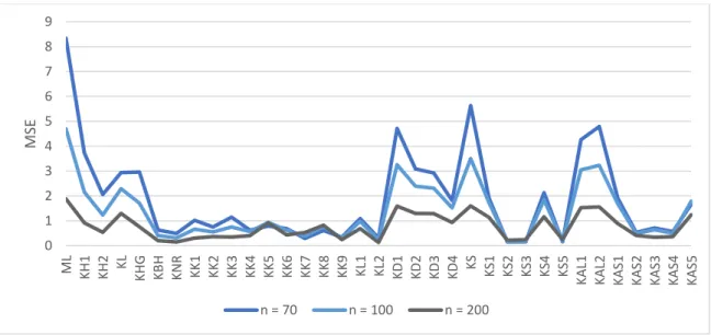
Figure 3.1

.Performance of estimators as a function of sample size for p = 4, ρ =0.95, intercept = 0

Figure 3.1 shows that all RR estimators outperform the ML estimator in the sense of

smaller MSE for different sample sizes and it is evident the advantage of using logistic ridge

regression estimators over ML estimator when explanatory variables are correlated.

0 1 2 3 4 5 6 7 8 9 ML _KH1 _KH2 KL _KHG _KBH R_KN _KK1 _KK2 _KK3 _KK4 _KK5 _KK6 _KK7 _KK8 _KK9 _KL1 _KL2 _KD1 _KD2 _KD3 _KD4 KS 1_KS _KS2 _KS3 _KS4 _KS5 KA L1 KA L2 KA S1 KA S2 KA S3 KA S4 KA S5 MSE n = 70 n = 100 n = 200

(20)

13

Furthermore, increasing sample size has a positive effect on the mean absolute percent

error (MAPE). In general, MAPE decreases as the number of observation increase with a few

exceptions. Graphical illustration of the performance based on MAPE for different sample sizes

with fixed p = 4, correlation coefficient 0.95 and intercept 0 is presented in the Figure 3.2.

Figure 3.2

. Performance of estimators as a function sample size for p = 4, ρ =0.95, intercept = 0

Figure 3.2 shows that all RR estimators outperform the ML estimator in terms of MAPE

for different sample sizes and it shows the advantage of using logistic ridge regression estimators

over ML estimator. The best RR estimators in terms of MAPE achieved when sample size is large,

in this case when n is 200.

3.2.2 Results as a function of ρ

It is easy to see that MSEs for estimators of

k

increases as correlation coefficient increases.

For smaller correlation coefficient (ρ = 0.75 and ρ = 0.85), the MSEs are almost the same for any

sample size, an intercept and number of parameters. For given n = 100 and intercept 0, performance

of estimators as a function of the correlation between the explanatory variables for p = 4 and p = 8

is provided in Figure 3.3 – 3.4 and Figure 3.5 - 3.6, respectively.

0 0.5 1 1.5 2 2.5 ML _KH1 _KH2 KL _KHG _KBH _KNR _KK1 _KK2 _KK3 _KK4 _KK5 _KK6 _KK7 _KK8 _KK9 KL1 KL2 KD1 KD2 KD3 KD4 KS 1KS KS2 KS3 KS4 KS5 KA L1 KA L2 KA S1 KA S2 KA S3 KA S4 KA S5 MAPE n = 70 n = 100 n = 200

(21)

14

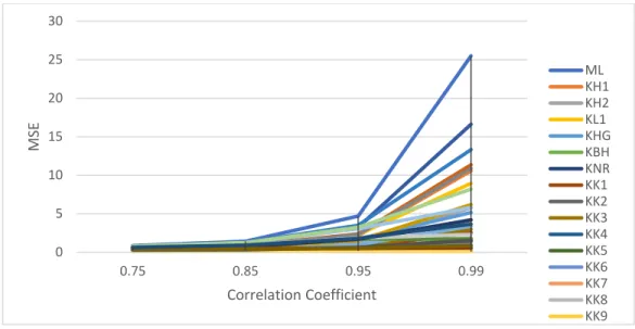
Figure 3.3.

Performance of the estimators as a function of ρ when p = 4, n = 100 and intercept = 0

Figure 3.4.

Performance of the selected estimators as a function of ρ when p = 4, n =100,intercept=0

0 5 10 15 20 25 30 0.75 0.85 0.95 0.99 MSE Correlation Coefficient ML KH1 KH2 KL1 KHG KBH KNR KK1 KK2 KK3 KK4 KK5 KK6 KK7 KK8 KK9 0 1 2 3 4 5 6 7 0.75 0.85 0.95 0.99 MSE Correlation Coefficient KL2 KBH KS2 KS3 KS5 KK1 KK9 KNR KAS3 KK3 KK4 KK6 KH2 KK2 KAS4

(22)

15

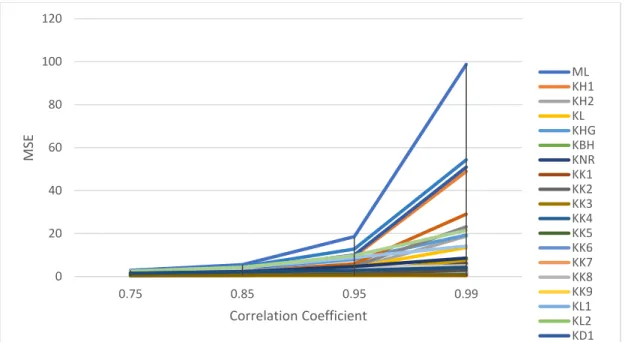
Figure 3.5.

Performance of the estimators as a function of ρ when p = 8, n = 100 and intercept = 0

Figure 3.6.

Performance of the selected estimators as a function of ρ when p = 8, n = 100 and

intercept = 0

0 20 40 60 80 100 120 0.75 0.85 0.95 0.99 MSE Correlation Coefficient ML KH1 KH2 KL KHG KBH KNR KK1 KK2 KK3 KK4 KK5 KK6 KK7 KK8 KK9 KL1 KL2 KD1 0 2 4 6 8 10 12 14 16 18 20 0.75 0.85 0.95 0.99 MSE Correlation Coefficient KH2 KBH KNR KK1 KK2 KK3 KK4 KK6 KK9 KL2 KS2 KS3 KS5 KAS3 KAS4

(23)

16

These figures show that as correlation increases the MSE also increases. Also, MSE of ML

estimator increases rapidly as correlation coefficient increase from 0.85 to 0.99. All the RR

estimators have smaller MSE compared with ML and they don’t change as rapidly as ML estimator.

3.2.3 Results as a function of p

Overall, the MSE increases when more explanatory variables are included, disregarding

the fact that changing the number of explanatory variables from 4 to 8 the number of observations

is also changes. For given n = 100, intercept 0, and correlation coefficients 0.95, performance of

estimators as a function of the number of explanatory variables for p = 4 and p = 8 is provided in

Figure 3.7.

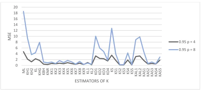
Figure 3.7

.Performance of the estimators as a function of p with ρ= 0.95, n= 100 and intercept = 0

From this figure 3.8, we observe that as the number of explanatory variables increases from

4 to 8, the MSE also increases. Also, as the number of explanatory variables increases proportion

for which ML estimator has bigger MSE than the other estimator decreases.

3.2.4 Results as function of the intercept

Since the value of the intercept is equal to the average value of the log odds ratio, then with

intercept equal to zero there is an equal probability of obtaining ones and zeros. With intercept

equal to 1 there is a greater probability of obtaining ones than zeros. Also, with intercept equal to

0 2 4 6 8 10 12 14 16 18 20 ML KH1 KH2 KL KHG KBH KN R KK1 KK2 KK3 KK4 KK5 KK6 KK7 KK8 KK9 KL1 2KL _{KD1 KD2 KD3 KD4} KS KS1 KS2 KS3 KS4 KS5 _KAL1 _KAL2 _KAS1 _KAS2 _KAS3 _KAS4 _KAS5 MSE ESTIMATORS OF K 0.95 p = 4 0.95 p = 8

(24)

17

-1 there is a greater probability of obtaining zeros than ones. For given n = 100, p = 4, and

correlation coefficients 0.95, performance of estimators as a function of the log odds ratio is

provided in Figure 3.8.

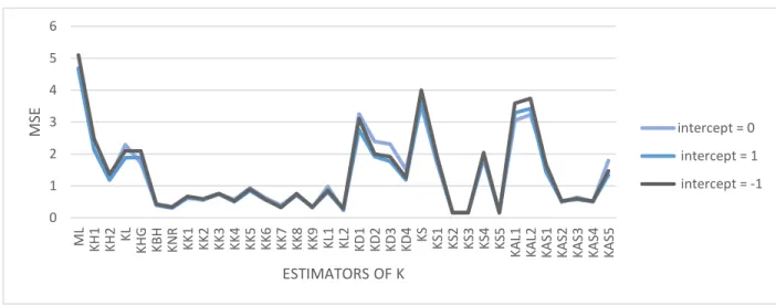
Figure 3.8

. Performance of the estimators as a function of the intercept when ρ = 0.95, n = 100 and

p = 4.

From Figure 3.8, we observe that changing the log odds from zero to 1 or -1 MSE increases

for the ML and the KD1 – KD3 and KAL1, KAL2. The MSEs for the other estimators are the same

or slightly decreases. Hence, these estimators are more robust to changes of the log odd ratio than

ML and the KD1 – KD3 and KAL1, KAL2.

3.3 Some Proposed New Estimators of k.

From the results analysis in section 3.2, it is evident that the following estimators: KHB, KNR,

KK2, KK4, KK6, KK7, KK9, KK12, KS2, KS5 are performing better than the rest of the estimators.

Thus, the following new estimators of

k

are proposed in this section:

1.

KN1 = Maximum (KHB, KNR, KK2, KK4, KK6, KK7, KK9, KK12, KS2, KS5)

2.

KN2 = Arithmetic mean of (KHB, KNR, KK2, KK4, KK6, KK7, KK9, KK12, KS2, KS5)

3.

KN3 = Median (KHB, KNR, KK2, KK4, KK6, KK7, KK9, KK12, KS2, KS5)

4.

KN4 = Harmonic mean (KHB, KNR, KK2, KK4, KK6, KK7, KK9, KK12, KS2, KS5)

0 1 2 3 4 5 6 ML _KH1 _KH2 KL _KHG _KBH R_KN _KK1 _KK2 _KK3 _KK4 _KK5 _KK6 _KK7 _KK8 _KK9 _KL1 _KL2 _KD1 _KD2 _KD3 _KD4 KS _KS1 _KS2 _KS3 _KS4 _KS5 KA L1 KA L2 KA S1 KA S2 KA S3 KA S4 KA S5 MSE ESTIMATORS OF K intercept = 0 intercept = 1 intercept = -1

(25)

18

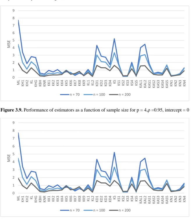
The MSEs values for n = 70, 100, and 200, ρ = 0.95 and p = 4 are reported for different values

of intercept in table A4. Also, performance of estimators including new estimators as a function of

sample size are plotted in Figures 3.9 – 3.11.

Figure 3.9.

Performance of estimators as a function of sample size for p = 4,ρ =0.95, intercept = 0

Figure 3.10

.Performance of estimators as a function of sample size for p = 4,ρ =0.95,intercept = 1

0 1 2 3 4 5 6 7 8 9 ML _KH1 _KH2 KL _KHG _KBH R_KN _KK1 _KK2 _KK3 _KK4 _KK5 _KK6 _KK7 _KK8 _KK9 _KL1 _KL2 _KD1 _KD2 _KD3 _KD4 KS _KS1 _KS2 _KS3 _KS4 _KS5 KA L1 KA L2 KA S1 KA S2 KA S3 KA S4 KA S5 KN 1 KN 2 KN 3 KN 4 MSE n = 70 n = 100 n = 200 0 1 2 3 4 5 6 7 8 9 ML _KH1 _KH2 KL _KHG _KBH _KNR _KK1 _KK2 _KK3 _KK4 _KK5 _KK6 _KK7 _KK8 _KK9 KL1 KL2 _KD1 _KD2 _KD3 _KD4 KS KS1 KS2 KS3 KS4 KS5 L1_KA _KAL2 _KAS1 _KAS2 _KAS3 _KAS4 _KAS5 KN 1 KN 2 KN 3 KN 4 MSE n = 70 n = 100 n = 200

(26)

19

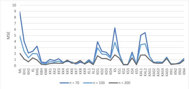
Figure 3.11

.Performance of estimators as a function of sample size for p= 4,ρ =0.95,intercept = -1

It appears from Figures 3.9 – 3.11 and Tables in A.4, that all new proposed estimators

performed better in the sense of smaller MSE compare to the rest of the estimators. The estimator,

KN3 performed the best among proposed five and rest of the estimators.

0 1 2 3 4 5 6 7 8 9 10 ML _KH1 _KH2 KL _KHG _KBH _KNR _KK1 _KK2 _KK3 _KK4 _KK5 _KK6 _KK7 _KK8 _KK9 KL1 KL2 _KD1 _KD2 _KD3 _KD4 KS KS1 2KS KS3 KS4 KS5 _KAL1 _KAL2 KA S1 KA S2 KA S3 KA S4 KA S5 KN 1 KN 2 KN 3 KN 4 MSE n = 70 n = 100 n = 200

(27)

20

CHAPTER IV

APPLICATION

To illustrate the findings of this thesis, we consider the data, which have been taken from

survey of 659 registered leisure boat owners in 23 counties of East Texas collected by Sellar, Stoll

and Chavas (1985). We consider the following logistic regression model

Y =

exp⁡(β₀+X₁β₁+X₂β₂+⁡X₃β₃+⁡X₄β₄+X₅β₅)

1+⁡exp⁡(β₀+X₁β₁+X₂β₂+⁡X₃β₃+⁡X₄β₄+X₅β₅)

,

(4.1)

where Y is defined as 0, if survey participant has not taken a recreational trip and 1, otherwise. X

1

is the facility's subjective quality ranking, X

2

is the respondent's taste for water-skiing, X

3

is travel

cost to Lake Conroe, X

4

is travel cost to Lake Somerville, X

5

is travel cost to Lake Houston. The

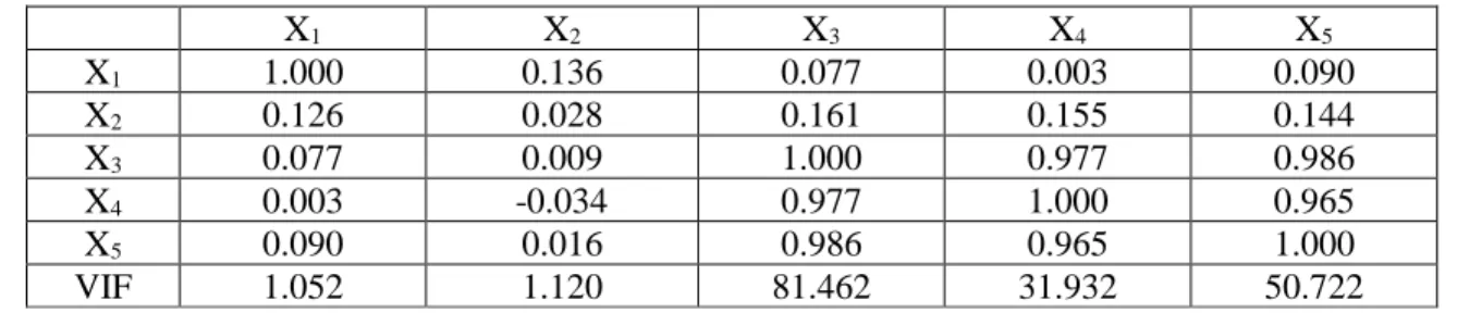
correlation matrix of the variables in model (4.1) is presented in Table 4.1 (see Shiferaw Gurmu,

1996)

Table 4.1

. Correlation among the variables with corresponding VIF

X

1

X

2

X

3

X

4

X

5

X

1

1.000

0.136

0.077

0.003

0.090

X

2

0.126

0.028

0.161

0.155

0.144

X

3

0.077

0.009

1.000

0.977

0.986

X

4

0.003

-0.034

0.977

1.000

0.965

X

5

0.090

0.016

0.986

0.965

1.000

VIF

1.052

1.120

81.462

31.932

50.722

It is observed from Table 4.1 that the explanatory variables X

3

, X

4

, X

5

are highly

correlated. Also, variance inflation factors for X

3

, X

4

, X

5

are 81, 31, and 50 respectively.

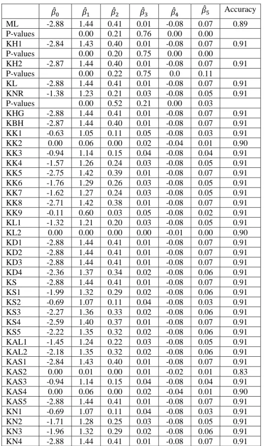
It implies the existence of multicollinearity problem in the data set. The estimated predicted proba

bility along with the ridge regression coefficients of the estimators are presented in Table 4.2. I als

o provided the p-values for testing the significance of regression parameters of the following estim

ators: ML, KH1, KH2 and KNR. From Table 4.2, we observed that all ridge regression estimators

have higher prediction accuracy than that of ML estimator, which supported our findings from sim

ulation study in Chapter 3.

(28)

21

Table 4.2.

The MSEs along with the ridge regression coefficients of the estimators

𝛽̂

0

𝛽̂

1

𝛽̂

2

𝛽̂

3

𝛽̂

4

𝛽̂

5

Accuracy

ML

-2.88

1.44

0.41

0.01

-0.08

0.07

0.89

P-values

0.00

0.21

0.76

0.00

KH1

-2.84

1.43

0.40

0.01

-0.08

0.07

0.91

P-values

0.00

0.20

0.75

0.00

KH2

-2.87

1.44

0.40

0.01

-0.08

0.07

0.91

P-values

0.00

0.22

0.75

0.0

0.11

KL

-2.88

1.44

0.41

0.01

-0.08

0.07

0.91

KNR

-1.38

1.23

0.21

0.03

-0.08

0.05

0.91

P-values

0.00

0.52

0.21

0.00

0.03

KHG

-2.88

1.44

0.41

0.01

-0.08

0.07

0.91

KBH

-2.87

1.44

0.40

0.01

-0.08

0.07

0.91

KK1

-0.63

1.05

0.11

0.05

-0.08

0.03

0.91

KK2

0.00

0.06

0.00

0.02

-0.04

0.01

0.90

KK3

-0.94

1.14

0.15

0.04

-0.08

0.04

0.91

KK4

-1.57

1.26

0.24

0.03

-0.08

0.05

0.91

KK5

-2.75

1.42

0.39

0.01

-0.08

0.07

0.91

KK6

-1.76

1.29

0.26

0.03

-0.08

0.05

0.91

KK7

-1.62

1.27

0.24

0.03

-0.08

0.05

0.91

KK8

-2.71

1.42

0.38

0.01

-0.08

0.07

0.91

KK9

-0.11

0.60

0.03

0.05

-0.08

0.02

0.91

KL1

-1.32

1.21

0.20

0.03

-0.08

0.05

0.91

KL2

0.00

-0.01

0.00

0.90

KD1

-2.88

1.44

0.41

0.01

-0.08

0.07

0.91

KD2

-2.88

1.44

0.41

0.01

-0.08

0.07

0.91

KD3

-2.88

1.44

0.41

0.01

-0.08

0.07

0.91

KD4

-2.36

1.37

0.34

0.02

-0.08

0.06

0.91

KS

-2.88

1.44

0.41

0.01

-0.08

0.07

0.91

KS1

-1.99

1.32

0.29

0.02

-0.08

0.06

0.91

KS2

-0.69

1.07

0.11

0.04

-0.08

0.03

0.91

KS3

-2.27

1.36

0.33

0.02

-0.08

0.06

0.91

KS4

-2.59

1.40

0.37

0.01

-0.08

0.07

0.91

KS5

-2.22

1.35

0.32

0.02

-0.08

0.06

0.91

KAL1

-1.45

1.24

0.22

0.03

-0.08

0.05

0.91

KAL2

-2.18

1.35

0.32

0.02

-0.08

0.06

0.91

KAS1

-2.84

1.43

0.40

0.01

-0.08

0.07

0.91

KAS2

0.00

0.01

0.00

0.01

-0.02

0.01

0.83

KAS3

-0.94

1.14

0.15

0.04

-0.08

0.04

0.91

KAS4

0.00

0.06

0.00

0.02

-0.04

0.01

0.90

KAS5

-2.88

1.44

0.41

0.01

-0.08

0.07

0.91

KN1

-0.69

1.07

0.11

0.04

-0.08

0.03

0.91

KN2

-1.71

1.28

0.25

0.03

-0.08

0.05

0.91

KN3

-1.96

1.32

0.29

0.02

-0.08

0.06

0.91

KN4

-2.88

1.44

0.41

0.01

-0.08

0.07

0.91

(29)

22

CHAPTER V

SUMMARY AND CORRESPONDING REMARKS

In this thesis, we investigated some ridge regression (RR) estimators for estimating the

ridge regression parameter

k

for logistic regression model when the explanatory variables are highly

correlated. Since a theoretical comparison among the estimators is not possible, a Monto Carlo

simulation study has been conducted to compare the performance of the proposed ridge regression

estimators. In simulation, we evaluated proposed estimators of

k

for different experimental

conditions: the degree of correlation, sample size, the number of independent variables, and the log

odds ratio. For each combination of parameters, we performed 2000 replications. The evaluation

of the performance of these estimators has been done by using the MSE, MAPE, the magnitude of

bias, and the proportion of times the ML outperforms the RR estimators.

The simulation results show that the increase of the correlation among the explanatory

variables and the number of independent variables have a negative effect on the performance of the

estimators, the MSE and MAPE increases. In most of the cases, RR estimators outperform ML

estimator even when the correlation between the explanatory variables are large. When the sample

size increases the MSEs as well as MAPE decreases for all estimators including ML estimator. The

analysis of the log odds ratio reveals that majority of estimators are robust to changes of the log

odds ratio with few exceptions. The top ten estimators of

k

from our simulation study are KHB,

KNR, KK2, KK4, KK6, KK7, KK9, KK12, KS2, KS5. Also, new proposed estimators based on

top ten estimators have performed well compared to other estimators. Furthermore, the analysis

from real data supported the results from simulation study to some extent.

(30)

23

The following estimators KBH, KNR, KK2, KK6, KK7, KL2, KS2, KS5, KN1, KN2, KN3

are recommending for the practitioners for using them when they analysis data with

multicollinearity problem.

We have considered the logistic regression model. As a future research, this can further be

extended for the following models:

(i)

Two parameters logistic regression model. That means, a model with both ridge

regression estimator and Liu (1993) estimator.

(ii)

Ridge Regression Based on Some Robust Estimators (see Samkar and Alpu, 2010).

(iii)

Ridge regression estimators for the restricted linear model.

(31)

24

REFERENCES

1.

Alkhamisi M.A., G. Shukur.A. (2007). “Monte Carlo study of recent ridge parameters”.

Communications in Statistics – Simulation and Computation, 36 (3), pp. 535-547.

2.

Alkhamisi M.A., Mahdi & Khalaf, Ghadban & Shukur, Ghazi. (2006). “Some Modifications for

Choosing Ridge Parameters”. Communications in Statistics. Theory and Methods. 35(11), pp.

2005-2020.

3.

Asar, Y and Genc, A. (2017). “A note on some new modifications of ridge estimators”. Kuwait J.

Sci. 44 (3)

pp. 75-82.

4.

Batah, F. S.M., Ramanathan, T.V., Gore, S.D. (2008). “The efficiency of modified Jack-knife and

ridge type regression estimators: a comparison”. Surveys in Mathematics and its Applications. 3,pp.

111 – 122.

5.

Dorugade A.V. (2013). “New ridge parameters for ridge regression”. Journal of the Association

of Arab Universities for Basic and Applied Sciences. 15, 94-99.

6.

Hocking R.R., F.M. Speed, M.J. Lynn. (1976) “A class of biased estimators in linear regression”.

Technometrics, 18 (4) , pp 425-437.

7.

Hoerl, Arthur E., and Robert W. Kennard (1970). “Ridge regression: Biased Estimation for

Nonorthogonal Problems”. Technometrics. 12(1), pp. 55 – 67.

8.

Hoerl, Arthur E., Robert W. Kannard & Kent F. Baldwin. (1975) “Ridge regression:some

simulations.” Communications in Statistics . 4(2), pp. 105 – 123.

9.

Kibria B. M. G. (2003). “Performance of Some New Ridge Regression Estimators” .

Communications in Statistics- Theory and Methods. 32(2), pp. 419 – 435.

10. Kibria, B. M. Golam and Banik, Shipra (2016). “Some Ridge Regression Estimators and Their

Performances.” Journal of Modern Applied Statistical Methods. 15(1), Article 12, pp. 206-238.

11. Lawless, J. F., Wang, P. (1976). “A simulation study of ridge and other regression estimators”.

Communications in Statistics—Theory and Methods. 5, pp. 307–323.

12. A. H. Lee & M. J. Silvapulle (1998). “Ridge estimation in logistic regression”. Communications in

Statistics - Simulation and Computation, 17(4), pp.1231-1257

13. Liu, K. (1993). “A new class of biased estimate in linear regression”. Communications in

Statistics: Theory and Methods. 22, pp. 393–402.

(32)

25

14. Lukman, A. F., Ayinde, K., & Ajiboye, A. S. (2017). “Monte Carlo study of some

classification-based ridge parameter estimators”. Journal of Modern Applied Statistical Methods, 16(1), pp.

428-451.

15. Månsson K., Shukur G. (2011).” On Ridge Parameters in Logistic Regression”. Communications

in Statistics - Theory and Methods . 40(18), pp. 3366-3381.

16.

Månsson, K, Shukur, G. and Kibria, B. M. G. (2017). “Performance of Some Ridge Regression

Estimators for the Multinomial Logit Model”. Communications in Statistics-Theory and

Methods.

17. Muniz, Gisela and Kibria, B.M. Golam (2009). “On Some Ridge Regression Estimators: An

Empirical Comparisons”. Communications in Statistics- Theory and Methods. 38 (3), pp. 621 - 630

18. Muniz, Gisela; Kibria, B.M. Goam; and Shukur, Ghazi. (2012). “On Developing Ridge Regression

Parameters: A Graphical investigation”. Department of Mathematics and Statistics. 10, pp. 1 – 25.

19. Nomura M.(1988) “ On the almost unbiased ridge regression estimator”. Communications in

Statistics - Simulation and Computation . 17(3), pp. 729 – 743.

20. Sellar, C., Stoll, J. R., and Chavas, J. P. (1985), “Validation of Empirical Measures of Welfare

Change: A Comparison of Nonmarket Techniques.” Land Economics, 61, 156-175.

21. Samkar, Hatice and Alpu, Ozlem (2010) "Ridge Regression Based on Some Robust Estimators,"

Journal of Modern Applied Statistical Methods. 9(2),Article 17, pp. 495-501

22. Schaefer R.L., L.D. Roi & R.A. Wolfe (1984).“A ridge logistic estimator”. Communications in

Statistics - Theory and Methods . 1391). pp. 100-112

23. Shiferaw Gurmu and Pravin K. Trivedi (1996). “Excess Zeros in Count Models for Recreational

Trips. Journal of Business & Economic Statistics”.14(4), pp. 469-47.

(33)

26

APPENDICES

Table A1.

Estimated MSEs, MAPEs, Bias and proportion of times in simulation when the ridge

regression estimator produces a higher MSE than the ML estimator of the proposed estimators

with intercept = 0 for the following cases:

p = 4, ρ =0.75

n = 70 n = 100 n = 200

MSE Bias MAPE Pr. MSE Bias MAPE Pr. MSE Bias MAPE Pr.

ML 1.40 0.00 0.91 0.00 0.84 0.00 0.72 0.00 0.36 0.00 0.48 0.00 KH1 0.75 0.20 0.65 0.02 0.49 0.16 0.54 0.03 0.26 0.10 0.40 0.04 KH2 0.47 0.37 0.52 0.04 0.33 0.31 0.45 0.05 0.19 0.20 0.34 0.07 KL 0.92 0.11 0.73 0.01 0.67 0.06 0.64 0.02 0.34 0.02 0.46 0.02 KHG 0.85 0.15 0.70 0.01 0.56 0.12 0.58 0.03 0.28 0.07 0.42 0.03 KBH 0.24 0.68 0.42 0.09 0.20 0.63 0.38 0.12 0.13 0.50 0.30 0.17 KNR 0.31 0.98 0.51 0.09 0.29 0.99 0.50 0.12 0.26 0.96 0.48 0.17 KK1 0.35 0.69 0.49 0.11 0.28 0.62 0.44 0.14 0.17 0.46 0.34 0.18 KK2 0.48 1.09 0.62 0.23 0.43 1.05 0.59 0.31 0.34 0.90 0.50 0.43 KK3 0.39 0.68 0.51 0.11 0.30 0.61 0.45 0.14 0.19 0.45 0.36 0.18 KK4 0.35 0.37 0.47 0.03 0.30 0.30 0.43 0.04 0.19 0.18 0.35 0.05 KK5 0.73 0.10 0.69 0.01 0.61 0.06 0.62 0.01 0.32 0.02 0.45 0.02 KK6 0.38 0.36 0.48 0.03 0.31 0.28 0.44 0.04 0.20 0.17 0.35 0.05 KK7 0.45 0.21 0.55 0.01 0.44 0.12 0.54 0.02 0.28 0.05 0.42 0.02 KK8 0.67 0.12 0.66 0.01 0.57 0.07 0.61 0.02 0.31 0.03 0.45 0.02 KK9 0.33 0.78 0.49 0.12 0.28 0.69 0.45 0.16 0.19 0.50 0.36 0.19 KL1 0.52 0.92 0.62 0.18 0.44 0.78 0.56 0.22 0.29 0.50 0.44 0.23 KL2 0.22 0.60 0.39 0.02 0.18 0.50 0.34 0.03 0.12 0.40 0.28 0.09 KD1 0.94 0.11 0.74 0.01 0.67 0.06 0.64 0.02 0.34 0.02 0.46 0.02 KD2 0.68 0.28 0.63 0.04 0.53 0.18 0.56 0.04 0.30 0.06 0.43 0.04 KD3 0.65 0.27 0.61 0.03 0.51 0.17 0.55 0.03 0.30 0.06 0.43 0.03 KD4 0.56 0.63 0.60 0.12 0.46 0.51 0.55 0.13 0.29 0.30 0.43 0.14 KS 1.23 0.03 0.86 0.01 0.77 0.02 0.69 0.01 0.35 0.01 0.47 0.02 KS1 0.92 0.08 0.75 0.01 0.65 0.05 0.64 0.02 0.32 0.02 0.45 0.02 KS2 0.23 0.43 0.38 0.02 0.24 0.30 0.39 0.03 0.19 0.15 0.35 0.04 KS3 0.24 0.41 0.39 0.02 0.24 0.29 0.40 0.03 0.19 0.14 0.35 0.04 KS4 0.93 0.08 0.76 0.01 0.66 0.05 0.64 0.02 0.32 0.02 0.45 0.02 KS5 0.24 0.41 0.39 0.02 0.24 0.29 0.39 0.03 0.19 0.14 0.35 0.04 KAL1 1.19 0.03 0.85 0.01 0.76 0.02 0.69 0.01 0.35 0.01 0.47 0.02 KAL2 1.21 0.03 0.85 0.01 0.77 0.02 0.69 0.01 0.35 0.01 0.47 0.02 KAS1 0.65 0.22 0.61 0.02 0.47 0.17 0.53 0.03 0.25 0.10 0.40 0.04 KAS2 0.59 1.38 0.72 0.32 0.56 1.35 0.69 0.43 0.48 1.21 0.63 0.60 KAS3 0.37 0.69 0.50 0.11 0.29 0.61 0.45 0.14 0.19 0.45 0.36 0.18 KAS4 0.48 1.09 0.62 0.23 0.43 1.05 0.58 0.31 0.34 0.90 0.50 0.43 KAS5 0.79 0.14 0.69 0.01 0.63 0.07 0.62 0.02 0.34 0.02 0.46 0.02

(34)

27

p = 4, ρ =0.85

n = 70 n = 100 n = 200

ML 2.37 0.00 1.17 0.00 1.42 0.00 0.93 0.00 0.60 0.00 0.61 0.00 KH1 1.18 0.16 0.78 0.01 0.76 0.14 0.65 0.01 0.37 0.10 0.47 0.02 KH2 0.67 0.31 0.59 0.02 0.47 0.26 0.51 0.02 0.25 0.19 0.39 0.03 KL 1.26 0.13 0.83 0.00 0.98 0.07 0.76 0.01 0.53 0.02 0.57 0.01 KHG 1.25 0.14 0.81 0.00 0.82 0.12 0.68 0.01 0.40 0.08 0.49 0.01 KBH 0.26 0.54 0.41 0.03 0.21 0.50 0.37 0.04 0.13 0.42 0.30 0.08 KNR 0.27 0.80 0.46 0.03 0.23 0.79 0.43 0.04 0.19 0.77 0.40 0.08 KK1 0.40 0.60 0.50 0.06 0.31 0.54 0.45 0.07 0.18 0.40 0.35 0.08 KK2 0.49 1.02 0.61 0.14 0.43 0.97 0.58 0.20 0.32 0.84 0.49 0.28 KK3 0.46 0.60 0.53 0.06 0.35 0.53 0.47 0.08 0.21 0.40 0.36 0.09 KK4 0.40 0.34 0.49 0.01 0.36 0.27 0.46 0.02 0.25 0.16 0.39 0.02 KK5 0.87 0.12 0.75 0.00 0.80 0.06 0.72 0.01 0.49 0.02 0.56 0.01 KK6 0.43 0.33 0.51 0.01 0.39 0.25 0.48 0.02 0.26 0.15 0.40 0.02 KK7 0.45 0.23 0.54 0.00 0.50 0.13 0.57 0.01 0.39 0.05 0.50 0.01 KK8 0.76 0.13 0.71 0.00 0.72 0.08 0.69 0.01 0.47 0.03 0.55 0.01 KK9 0.32 0.73 0.48 0.06 0.29 0.64 0.45 0.08 0.20 0.46 0.36 0.09 KL1 0.57 0.88 0.63 0.11 0.50 0.73 0.59 0.14 0.34 0.45 0.47 0.13 KL2 0.23 0.66 0.40 0.01 0.18 0.55 0.34 0.01 0.12 0.41 0.28 0.04 KD1 1.45 0.10 0.90 0.00 1.07 0.06 0.79 0.01 0.54 0.02 0.58 0.01 KD2 0.98 0.25 0.72 0.01 0.81 0.16 0.68 0.02 0.47 0.06 0.53 0.01 KD3 0.90 0.24 0.70 0.01 0.78 0.15 0.66 0.01 0.46 0.05 0.53 0.01 KD4 0.68 0.60 0.64 0.07 0.60 0.48 0.61 0.08 0.38 0.26 0.48 0.07 KS 1.96 0.02 1.07 0.00 1.25 0.02 0.87 0.01 0.56 0.01 0.59 0.01 KS1 1.23 0.08 0.88 0.00 0.95 0.05 0.77 0.01 0.50 0.02 0.56 0.01 KS2 0.21 0.43 0.36 0.00 0.23 0.30 0.38 0.01 0.23 0.15 0.38 0.01 KS3 0.22 0.41 0.37 0.00 0.24 0.29 0.39 0.01 0.23 0.15 0.39 0.01 KS4 1.27 0.07 0.89 0.00 0.97 0.05 0.77 0.01 0.50 0.02 0.56 0.01 KS5 0.22 0.41 0.37 0.00 0.24 0.29 0.39 0.01 0.23 0.15 0.39 0.01 KAL1 1.83 0.03 1.04 0.00 1.22 0.02 0.86 0.01 0.56 0.01 0.59 0.01 KAL2 1.88 0.03 1.05 0.00 1.23 0.02 0.87 0.01 0.56 0.01 0.59 0.01 KAS1 0.90 0.19 0.71 0.01 0.70 0.15 0.63 0.01 0.37 0.10 0.47 0.02 KAS2 0.57 1.32 0.70 0.20 0.53 1.27 0.67 0.28 0.45 1.16 0.61 0.43 KAS3 0.40 0.61 0.51 0.06 0.33 0.53 0.46 0.08 0.20 0.40 0.36 0.10 KAS4 0.47 1.03 0.61 0.14 0.43 0.97 0.58 0.20 0.32 0.84 0.49 0.28 KAS5 1.00 0.15 0.76 0.00 0.90 0.08 0.73 0.01 0.52 0.02 0.57 0.01

(35)

28

p = 4, ρ =0.95

n = 70 n = 100 n = 200

(36)

29

p = 4, ρ =0.99

n = 70 n = 100 n = 200

(37)

30

p = 8, ρ =0.75

n = 70 n = 100 n = 200

MSE Bias MAPE Pr. MS

E Bia

s MAPE Pr. MSE Bias MAPE Pr.

ML 208.80 0.00 2.22 0.00 2.87 0.00 1.29 0.00 1.04 0.00 0.80 0.00 KH1 3.38 0.20 1.28 0.00 1.62 0.18 0.95 0.00 0.70 0.13 0.65 0.00 KH2 1.21 0.47 0.80 0.00 0.72 0.43 0.64 0.00 0.38 0.33 0.48 0.00 KL 2.43 0.22 1.17 0.00 1.74 0.13 1.01 0.00 0.89 0.04 0.74 0.00 KHG 4.10 0.13 1.45 0.00 2.01 0.10 1.07 0.00 0.83 0.07 0.71 0.00 KBH 0.39 0.82 0.49 0.00 0.28 0.81 0.43 0.00 0.18 0.72 0.35 0.01 KNR 0.35 1.13 0.51 0.00 0.29 1.20 0.48 0.00 0.25 1.26 0.46 0.01 KK1 0.47 0.96 0.55 0.00 0.35 0.92 0.49 0.01 0.23 0.77 0.39 0.02 KK2 0.61 1.85 0.73 0.03 0.56 1.83 0.69 0.07 0.48 1.71 0.64 0.23 KK3 0.62 0.81 0.60 0.00 0.43 0.78 0.52 0.00 0.26 0.64 0.41 0.01 KK4 0.57 0.58 0.60 0.00 0.52 0.47 0.57 0.00 0.39 0.30 0.49 0.00 KK5 1.71 0.23 1.05 0.00 1.60 0.11 1.01 0.00 0.89 0.03 0.75 0.00 KK6 0.69 0.52 0.65 0.00 0.62 0.42 0.62 0.00 0.44 0.26 0.52 0.00 KK7 0.70 0.49 0.67 0.00 0.83 0.27 0.74 0.00 0.69 0.09 0.67 0.00 KK8 1.49 0.27 0.98 0.00 1.46 0.13 0.96 0.00 0.87 0.04 0.74 0.00 KK9 0.45 1.49 0.61 0.01 0.39 1.36 0.56 0.02 0.29 1.07 0.46 0.06 KL1 0.65 1.92 0.76 0.03 0.59 1.74 0.70 0.06 0.45 1.32 0.59 0.16 KL2 0.36 1.22 0.53 0.00 0.27 0.93 0.44 0.00 0.19 0.61 0.36 0.00 KD1 2.95 0.18 1.28 0.00 1.93 0.11 1.06 0.00 0.92 0.04 0.75 0.00 KD2 1.72 0.36 0.96 0.00 1.33 0.24 0.87 0.00 0.78 0.10 0.69 0.00 KD3 1.29 0.44 0.84 0.00 1.10 0.30 0.79 0.00 0.72 0.12 0.66 0.00 KD4 0.69 1.29 0.70 0.01 0.63 1.10 0.66 0.03 0.48 0.72 0.56 0.06 KS 8.47 0.05 1.69 0.00 2.52 0.03 1.22 0.00 0.99 0.01 0.78 0.00 KS1 2.39 0.16 1.23 0.00 1.84 0.09 1.06 0.00 0.89 0.04 0.74 0.00 KS2 0.37 0.75 0.49 0.00 0.40 0.51 0.50 0.00 0.41 0.25 0.51 0.00 KS3 0.39 0.70 0.50 0.00 0.43 0.49 0.52 0.00 0.42 0.24 0.52 0.00 KS4 2.48 0.16 1.25 0.00 1.86 0.09 1.07 0.00 0.89 0.04 0.74 0.00 KS5 0.39 0.70 0.50 0.00 0.42 0.49 0.52 0.00 0.42 0.24 0.52 0.00 KAL1 7.47 0.07 1.60 0.00 2.43 0.04 1.20 0.00 0.98 0.01 0.78 0.00 KAL2 7.69 0.06 1.62 0.00 2.46 0.03 1.20 0.00 0.98 0.01 0.78 0.00 KAS1 1.91 0.26 1.06 0.00 1.42 0.20 0.91 0.00 0.69 0.13 0.64 0.00 KAS2 0.78 2.36 0.86 0.04 0.75 2.35 0.85 0.11 0.71 2.29 0.82 0.41 KAS3 0.51 0.84 0.57 0.00 0.40 0.79 0.51 0.00 0.26 0.65 0.41 0.01 KAS4 0.60 1.86 0.72 0.03 0.56 1.83 0.69 0.07 0.48 1.71 0.64 0.23 KAS5 1.72 0.27 1.02 0.00 1.55 0.15 0.97 0.00 0.88 0.05 0.73 0.00

(38)

31

p = 8, ρ =0.85

n = 70 n = 100 n = 200

ML 4369.38 0.00 5.59 0.00 5.53 0.00 1.77 0.00 1.82 0.00 1.05 0.00 KH1 6.19 0.15 1.70 0.00 2.96 0.13 1.27 0.00 1.12 0.10 0.81 0.00 KH2 2.17 0.34 1.03 0.00 1.26 0.31 0.82 0.00 0.54 0.26 0.56 0.00 KL 3.16 0.23 1.31 0.00 2.59 0.14 1.22 0.00 1.36 0.05 0.90 0.00 KHG 7.20 0.11 1.87 0.00 3.49 0.09 1.40 0.00 1.29 0.07 0.88 0.00 KBH 0.62 0.58 0.59 0.00 0.40 0.58 0.49 0.00 0.21 0.54 0.36 0.00 KNR 0.45 0.79 0.53 0.00 0.29 0.85 0.44 0.00 0.18 0.92 0.37 0.00 KK1 0.75 0.72 0.64 0.00 0.47 0.72 0.53 0.00 0.25 0.65 0.40 0.00 KK2 0.62 1.58 0.70 0.01 0.55 1.65 0.67 0.02 0.46 1.58 0.61 0.08 KK3 1.06 0.61 0.73 0.00 0.63 0.60 0.59 0.00 0.31 0.55 0.44 0.00 KK4 0.72 0.48 0.66 0.00 0.67 0.39 0.64 0.00 0.49 0.26 0.55 0.00 KK5 1.68 0.28 1.04 0.00 1.99 0.13 1.13 0.00 1.37 0.04 0.92 0.00 KK6 0.88 0.43 0.73 0.00 0.81 0.35 0.70 0.00 0.56 0.23 0.58 0.00 KK7 0.58 0.55 0.61 0.00 0.81 0.30 0.72 0.00 0.88 0.11 0.76 0.00 KK8 1.42 0.31 0.95 0.00 1.75 0.15 1.06 0.00 1.30 0.05 0.90 0.00 KK9 0.43 1.32 0.58 0.00 0.38 1.24 0.54 0.01 0.28 0.99 0.46