Post selection shrinkage estimation for high-dimensional data analysis By: Xiaoli Gao, S. E. Ahmed, Yang Feng
This is the peer reviewed version of the following article:
Gao, X.L., Ahmed, S.E. and Feng, Y. (2017). (Discussion paper) Post Selection Shrinkage Estimation for High Dimensional Data Analysis, Applied Stochastic Models in Business and Industry, 33(2), 97-120. doi:10.1002/asmb.2193,
which has been published in final form at http://dx.doi.org/10.1002/asmb.2193 . This article may be used for non-commercial purposes in accordance with Wiley Terms and Conditions for Self-Archiving.
***© Wiley. Reprinted with permission. No further reproduction is authorized without written permission from Wiley. This version of the document is not the version of record. Figures and/or pictures may be missing from this format of the document. ***
Abstract:
In high-dimensional data settings where p ≫ n, many penalized regularization approaches were studied for simultaneous variable selection and estimation. However, with the existence of covariates with weak effect, many existing variable selection methods, including Lasso and its generations, cannot distinguish covariates with weak and no contribution. Thus, prediction based on a subset model of selected covariates only can be inefficient. In this paper, we propose a post selection shrinkage estimation strategy to improve the prediction performance of a selected subset model. Such a post selection shrinkage estimator (PSE) is data adaptive and constructed by shrinking a post selection weighted ridge estimator in the direction of a selected candidate subset. Under an asymptotic distributional quadratic risk criterion, its prediction performance is explored analytically. We show that the proposed post selection PSE performs better than the post selection weighted ridge estimator. More importantly, it improves the prediction
performance of any candidate subset model selected from most existing Lasso-type variable selection methods significantly. The relative performance of the post selection PSE is demonstrated by both simulation studies and real-data analysis.
Keywords:asymptotic risk | lasso | ridge regression | (positive) shrinkage estimation | post selection | sparse model
Articles:
1 Introduction
Many high-dimensional data arise in biological, medical, social, and economical studies. Because of the trade-off between model complexity and model prediction, the statistical
inference of model selection becomes extremely important and challenging in high-dimensional data analysis. Consider a classical high-dimensional linear regression model with ith observed response variable yi and covariates xijs,
(1.1)
where ϵis is independent and identically distributed random errors with center 0 and variance σ2. Without loss of generality, we do not include the intercept in the model by assuming all data have been centered. Here, the subscript n in pn indicates that the number of coefficients may increase with the sample size n. Such a notation will be used throughout the paper without further explanation.
Over the past two decades, many penalized regularization approaches have been developed to do variable selection and estimation simultaneously. Among them, the Lasso [1] is one of the most popular approaches because of its convexity and computation efficiency. In general, the Lasso penalty tends to select an over-fitted model because it penalizes all coefficients equally [2]. Many endeavors have been undertaken to improve the Lasso to reach both variable selection consistency and the estimation consistency. To list a few, smoothly clipped absolute deviation [3, 4], adaptive Lasso [5] and minimax concave penalty [6], among others. An overview of variable selection in high-dimensional feature space can be found in [7].
In order to have nice estimation and selection properties, most Lasso-type penalties make some important assumptions about both true model and designed covariates. For example, the true model is often assumed to be sparse, insofar that (i) most βjs are zeros except for a few ones and (ii) all those nonzero βj's are larger than an inflated noise level, with
[8]. Additional assumptions made on the designed covariates include the adaptive irrepresentable condition and the restricted eigenvalue conditions. For detailed information, we refer to [9], [10], and [11].
However, those conditions are somewhat restrictive and are not judiciously justified in real applications. Consequently, Lasso and its generalizations may have lower prediction efficiency once those assumptions are violated. To fix the idea, we take the sparse model assumption (ii) as an example. Suppose we can divide the index set {1,…,pn} into three disjoint subsets: S1, S2, and S3. In particular, S1includes indexes of nonzero βi's which are moderately large and easily detected; S3 includes indexes with only zero coefficients; S2, being the intermediate, includes indexes of those nonzero βj with weak but nonzero effects. Thus, S1 is able to be detected using some existing variable selection techniques, while S2 may not be separated from S3 in general using existing Lasso-type methods. A more detailed description can be found in [8]. Following the spirit of model parsimony, covariates in S1 are kept in the model, and some or all covariates in S2 are left aside with ones in S3. Author in [12] has showed using simulation studies that such a Lasso estimate often performs worse than the post selection least squares estimate. To improve the prediction error of a Lasso-type variable selection approach, some (modified) post least squares estimators are studied in [13] and [14]. However, this work still assume the
irrepresentable condition, and those post estimations are only based upon the chosen subset after the Lasso. Consequently, the simultaneous weak effects in S2 are still ignored. An ideal strategy would be able to incorporate the joint contribution from covariates in S2, even though a
Let us consider an extreme case where S1 is a null set and p is fixed. It has been studied extensively that shrinkage estimators can have uniformly smaller risk compared with the ordinary maximum likelihood estimators (MLEs) since the discussion papers in [15] and [16]. The relative risk properties of shrinkage estimators were also investigated in low-dimensional regression models under a restricted linear submodel space. See, for example, [17-20] and many others.
However, in high-dimensional settings where p > n, a priori information on S1 is not guaranteed, not mentioning the existence of an MLE. Thanks to the existing variable selection techniques, an estimated candidate subset is selected. Once is obtained, the next question we want to ask is: can we construct a post selection shrinkage estimate to improve the risk of the post selection least squares estimators?
As we know, ridge regression [21, 22] has been widely used when the design matrix is ill-conditioned such that a regular MLE is not available. In this paper, we follow the model
parsimony spirit and extend shrinkage estimation to the high-dimensional data setting using both ridge penalty and Lasso-type penalty separately. In particular, we use a ridge penalty to construct a data-adaptive post selection shrinkage estimator (PSE) to improve the risk of a post selection least squares estimator based upon a Lasso-type variable selection result.
We summarize our main contributions as follows:
1. We propose a post selection shrinkage strategy to improve the risk of the Lasso-type estimators in high-dimensional settings. This post selection shrinkage strategy is data adaptive and has some practical applications, especially when an ‘important’ subset is generated and some covariates with joint weak effects are not selected.
2. We investigate the asymptotic risk of the proposed PSEs. Corresponding asymptotic properties of a predecessor generating those PSEs are also investigated under some regularity conditions.
The rest of the paper is organized as follows. In Section 2, we describe some preliminary model information involved in building a PSE. As preparation, we introduce some sparsity definitions under certain signal strength levels. Some existing variable selection results from Lasso are also summarized in this section. We propose three steps in constructing the shrinkage strategy in Section 3. In Section 4, we investigate some asymptotic properties of those post selection estimators during three steps in Section 3. We first investigate some asymptotic normality properties of the designed weighted ridge (WR) estimators under some conditions. Then, we investigate the asymptotic distributional risks of the linear combination of the proposed PSEs. In Sections 5 and 6, we perform some numerical studies using some simulated examples and a real-data application, respectively. We summarize the paper with some discussions in the final section. All proofs are given in the Appendix.
Let be the true coefficie ts vector in model (1.1). For any
subset S⊂{1,…,pn} with a cardinal value |S|, denote a subvector of β∗ indexed by S. Similar subscripts are used for other submatrices and subvectors.
2.1 Model sparsity and signal strength
As introduced in the previous section, the effect of all pn covariates is characterized into three categories based upon their signal strength: important covariates with strong effects in S1, covariates with no effect in S3, and an intermediate group in S2 with joint weak effects. In particular, those signal strength assumptions of the true model are made explicitly as follows: (A1) There exists a positive constant c1, such that for ∀j∈S1;
(A2) The parameter vector β∗ satisfies that for some 0 < τ < 1, where ∥·∥ is the ℓ2 norm;
(A3) , for ∀j∈S3.
Assumptions (A1–A3) specify those signal strength levels in the strong signals set S1, weak signals set S2, and sparse signal set S3 explicitly. In particular, (A2) indicates that joint weak effects in only grow with n at a certain rate, even though the dimension pn grows with n fast. For example, if (A1) holds for some c1 > 0 and we
let for j∈S2 with |S2| < n, then even
though pn = O(exp(n2τ)).
Most existing high-dimensional sparse models investigate the variable selection consistency by only considering the existence of the strong signals in (A1) and sparse signals in (A3). There is very limited work assuming the existence of weak signals in S2. For example, besides a strong signal set in (A1), [23] does not separate S2 and S3 and makes an alternative sparse model assumption,
(A2') for some .
In their work, some sufficient conditions are investigated under which the Lasso can select the strong signal set S1 consistently, following the spirit of the model parsimony.
Our weak and sparse conditions in (A2–A3) are different from the sparse condition in (A2') where S2 and S3 are not separated. If we replace (A2) by (A2') in our signal strength assumptions, then (A2) becomes , the joint effects in S2 being bounded uniformly. Thus, a true model under (A2') only is less sparse than one under (A3) only but more sparse than one in both (A2) and (A3). On the contrary, a sparse model under both (A2) and (A3) includes the most weak signals; a sparse model under (A3) only does not have any weak signals, while a sparse model under (A2') only is in the middle.
As discussed in Section 1, a penalized least squares (PLS) estimator is often adopted to select a parsimonious model for a high-dimensional regression model in (1.1),
(2.1)
where pλ(βj) is the penalty term on βj with a tuning parameter controlling the size of selected candidate subset model. For example, the Lasso takes pλ(βj) = λ|βj|, and the adaptive Lasso takes pλ(βj) = λ|βj|/|wj|, where wj can be taken as an initial estimator of βj. The size of selected subset model depends strongly on the choice of tuning parameters in (2.1). As pointed out by [8], one turns to ignore weak signals in S2together with S3 and select a candidate subset model with only strong signals in S1, following the model parsimony spirit.
If we let index an active subset from (2.1), then a data-adaptive candidate subset model is produced such that
(2.2)
Denote the response vector y = (y1,…,yn)′, all covariates vectors xj = (x1j,…,xnj)′ for j = 1,…,pn, and the design matrix . Without loss of generality, we rearrange the designed vectors such that , where XS is the submatrix consists of vectors indexed by S⊂{1,…,pn}. Next we give two scenarios where S2 cannot be separated from S3.
Case 1. ([24]) Consider an orthonormal design with X′X/n = In and ϵ ∼ N(0,In). The PLS with Lasso penalty provides a soft-threshold estimator with and 0,
for and , respectively. Here, is the least
squares solution, and sgn(·) is the sign mapping function.
If for some c > 0, then ; that
is, for j ∉ S1. Thus, all weak signals in S2 are omitted together with sparse signals in S3 using the Lasso approach.
Case 2. ([25]) Consider a non-singular design such that the smallest eigenvalue of is larger than some positive constant c. If there exists some j∈S2 such that |β0j| < |gj(λ)|,
where with ej being the jth column of the identity matrix, then . Thus, S2 and S3 cannot be separated using the Lasso. Some post selection estimators were proposed to improve the prediction performance of the PLS estimator. For example, under some regularity conditions, [13] and [14] studied some post selection least square estimators,
(2.3)
Here, we denote such a post selection least squares estimator as a restricted estimator (RE), written as in this paper. For notation's convenience, we omit the phase of ‘post selection’ in some future short notations without causing any confusion.
When S1 and S2 are not separable, we tend to select the important subset , such
that for a large enough λ, or for a smaller λ, following the spirit of model parsimony. Although is more estimation efficient than , the prediction risk of can still be high because many weak signals in S2 are ignored in . Our interest is to improve the risk performance of given in (2.3) by picking up some information from , a complement subset of the selected candidate submodel.
2.3 Some additional notations
Based upon a subset partition S1,S2,S3, we can partition the true parameters , without loss of generality. Some notations are shortened for notation's simplicity such
that for k = 1,2 and 3. Similar notations are also adopted for other subvectors and matrices. For example, after the same partition, the design matrix can be written as X = (X1,X2,X3). We also write X = (Z,X3) with Z = (X1,X2). The row vector of Z is
denoted as for 1≤i≤n.
We denote pk = |Sk| for 1≤k≤3 and pn = p1 + p2 + p3. In this paper, we allow to be very large but restrict q = p1 + p2≤n such that Σn = n − 1Z′Z is non-singular. If Σn is singular, then a generalized inverse matrix is adopted when needed in computations. Some other submatrices of Σn are defined as follows:
(2.4)
Let U = (X2,X3) be a n × (pn − p1) submatrix of X. Then, another partition is written as X = (X1,U). Let . Then, U′M1U is a (pn − p1) × (pn − p1) dimensional singular matrix with rank . We denote as all kn positive eigenvalues of U′M1U.
3 Post selection shrinkage estimation strategy
We propose a high-dimensional post selection shrinkage estimation strategy based upon the following three steps:
Step 1: Obtain a data-adaptive candidate subset following a model parsimony spirit and construct a post selection least square estimator using (2.3);
Step 2: Obtain a post selection WR estimator, , using a threshold ridge
penalty to be introduced and a submodel selected from Step 1;
Step 3: Obtain a PSE by shrinking from Step 2 in the direction of from Step 1. The post selection WR estimator in Step 2 can handle three scenarios simultaneously: (a) the sparsity in high-dimensional data analysis; (b) the strong correlation among covariates; and (c) the jointly weak contribution from some covariates.
Remark 1. This post selection shrinkage estimation is expected to improve the risk performance on the selected submodel once a variable selection approach in Step 1 tends to select those and only those variables with strong signal strength, that is, or . However, if the model parsimony spirit is not followed and λ in (2.1) is too small such that , this post selection shrinkage estimation is not suggested. Therefore, the effect of the PSE is data adaptive and depends on .
As a preparation, we first construct a post selection WR estimation based upon . This post selection weight ridge estimation itself is constructed from two steps introduced in
Section 'Weighted ridge estimation' and 'Post selection shrinkage estimation'. 3.1 Weighted ridge estimation
Once is obtained from Step 1, we seek to minimize a penalized objective function with a ridge penalty on coefficients in ,
(3.1)
where rn > 0 is a tuning parameter controlling the penalty effect on . Then, a post selection
WR estimator is obtained from,
where I(·) is the indicator function and an is a threshold parameter. Thus, we obtain estimators of the weak signal subset
(3.3) and of the sparse subset
(3.4)
Our post selection strategy is only applied when the threshold parameter an satisfies and . In particular, we set
(3.5)
Remark 2. We call a post selection WR estimator from two facts: (i) we only
penalize parameters in instead of the entire coefficients vector βn, and (ii) the threshold step in (3.2) can be interpreted as a WR penalty in (3.1), where wj = 0 and 1
for and .
Remark 3. Similar to the discussion in Remark 2, we can also understand the post selection step into the WR estimator, with wj = ∞ for . We do not enforce an
additional ridge penalty on to reduce some unnecessary biases during the WR step. This is different from the post selection threshold regression studied in [26], where the ℓ2 penalty is applied on the entire βn equally.
Remark 4. The idea of the WR regression is connected to the regularization after retention framework proposed in [27]. In that framework, a retention step is conducted to find the important set with large marginal-correlation coefficients with the response. Then, a regularization step is conducted by a penalized least square with L1 regularization only on the covariates that are not in . Compared with that framework, the current framework focused more on prediction by using the ridge penalty, and the estimate is also different.
Notice that for every selected candidate subset , depends
on rn and depends on both rn and an. For convenience, we omit those tuning parameters and denote above post selection WR estimators as and , respectively. 3.2 Post selection shrinkage estimation
Now, we are ready to propose a shrinkage estimation based upon two post selection estimators: and .
An initial PSE is defined as
(3.6) where and are given by
(3.7)
where . If σ2 is unknown, it is replaced by a consistent estimator . In the numerical studies, σ2 is replaced by , and a generalized inverse is used if is not singular.
Observing from (3.6) and (3.7), signs of two estimators of can be reversed if is too small such that . It is possible because consists of nuisance parameters, and over-shrinkage can occur for a large rn in the WR step. Thus, we also suggest to modify (3.6) as the following post selection PSE,
(3.8)
Remark 5. Our proposed post selection shrinkage estimation and the classical shrinkage estimation bear some resemblance but are different because of two facts: (i) Post selection shrinkage estimation is associated with a selected candidate subset and has some flexibility of adjusting the shrinkage strength data adaptively because depends on tuning
parameters an and rn; (ii) Post selection shrinkage estimation uses an initial ridge shrinkage step and is tailored for the high-dimensional settings where multiple covariates tend to be correlated and function jointly.
4 Asymptotic properties
In order to investigate some asymptotic properties of the proposed post selection estimators, we first make following assumptions on the random error, U′M1U, and the model sparsity. One can review some notations at the end of Section 2.
(B1) The random error ϵi ∼ N(0,σ2).
(B2) where τ < η≤1 for τ in (A2). (B3)log(pn) = O(nν) for 0 < ν < 1.
(B4) There exists a positive definite matrix Σ such that , where eigenvalues of Σ satisfy 0 < ρ1 < ρΣ < ρ2 < ∞.
Here, condition (B1) can be relaxed to a symmetric distribution with some finite moments. To simplify our theoretical investigations and handle the ultra high dimensionality, we only restrict our studies to normal random error in this paper. Condition (B2) guarantees that the positive eigenvalues of the redundant cannot be too small with a rate associated with the weak signals strength in S2. Condition (B3) permits the ultra-high dimensionality such that the number of variables can grow with sample size at an almost exponential rate. Condition (B4) is the regularity condition for . This condition is made in order to obtain the asymptotic normality the WR estimator.
4.1 Asymptotic properties of the weighted ridge estimator
We have the following asymptotic properties of the WR estimator .
Theorem 1. Suppose the sparse model in (1.1) satisfies signal strength assumptions in (A1–A3) and model assumptions in (B1–B3). If we choose for some constant c2 > 0 and an defined in (3.5) with α < (η − ν − τ)/3, then in (3.3) satisfies
(4.1) where τ, η, and ν are defined in (A2), (B2), and (B3), respectively.
Theorem 1 is similar to the variable selection result in [28]. We postpone the detailed proof to the Appendix. It tells us that the WR estimator is able to single out the sparse set S3 with a large probability, if S1 is pre-selected in advance such that . For
example, [23] argued that S1 can be recovered with a large probability under the sparse Riesz condition (SRC) with rank p1. Here, a design matrix X satisfies the SRC with rank q and spectrum bounds 0 < c∗ < c∗ < ∞ if
(4.2)
Lemma 1. Consider the Lasso solution for linear model (1.1) with ϵi ∼ N(0,σ2). Suppose (A1) and (B1) are satisfied, and the sparse condition (A2') holds for some ,
and the design matrix X satisfies the SRC with rank p1 in (4.2). Then, generated from a PLS with the Lasso penalty in (2.1) satisfies
Lemma 1 is a direct result from Theorem 2 in [23]. Here, the tuning parameter in (2.1) is chosen such that . Lemma 1 indicates that those and only those strong signals in S1 are included in while using the Lasso under sufficient conditions.
In Lemma 1, we have . The signal of each individual coefficient is trivial if such a joint effect is uniformly distributed on pn − p1 coefficients when pn ≫ n. However, if this joint effect is only distributed on a much smaller number of coefficients, each individual effect may not be negligible. In particular, if we let both (A2') and (A3) hold, then . Thus, (A2) also holds. Combing Lemma 1 and Theorem 1, we have the following result directly.
Corollary 1. Suppose all conditions in both Lemma 1 and Theorem 1 hold. Then, we have
(4.3)
Corollary 1 indicates that is able to be recovered if an additional WRs step is used post the Lasso under some sufficient conditions. We skip the proof because this is a direct result from Lemma 1 and Theorem 1.
However, Corollary 1 still requires a SRC condition. Although may not be guaranteed when a SRC condition is not satisfied, we may have
(4.4) Thus, we have similar but weaker result.
Corollary 2. Suppose all conditions in Theorem 1 hold, and satisfies (4.4). Then, we have
(4.5)
Corollary 2 can be interpreted by treating as a new S1 and as a new S2.
The asymptotic properties in Theorem 1 and its derivatives in Corollary 1 and 2 are important for establishing the efficiency of and .
Theorem 2. Let for any (p1n + p2n) × 1 vector dn satisfying ∥dn∥≤1. Suppose assumptions (B1–B4) hold. Consider a sparse model with signal strength under (A1), (A3), and
(A2) with 0 < τ < 1/2. Suppose a pre-selected model such as is obtained with probability 1. If we choose rn as in Theorem 1 with α < {(η − ν − τ)/3,1/4 − τ/2}, then we have the asymptotic normality,
(4.6)
Theorem 2 studies the asymptotic normality of the WR estimator, . In addition, has the same estimation efficiency as one from a restricted least square estimator as if is given as a priori. However, the result holds if and rn is chosen appropriately. More importantly, the strong signal set S1 is detected with a large probability in advance. This can be guaranteed under Lemma 1.
4.2 Asymptotic distributional risk analysis
In this section, we provide the relative performance of the post selection shrinkage estimation regarding the asymptotic distribution risk (ADR) introduced in [29]. For simplicity and notation's convenience, we focus on the ADR analysis by assuming , following the spirit of model parsimony. If , a similar analysis can be carried out by
redefining , as discussed in Section 4.1. Together with the results in Theorem 1, such that , S3 is also removed from the PSE with a large probability. Thus, the risk analysis in this section will be conducted by assuming both S1 and S3 are known in advance.
Definition 1. For any estimator and p1n − dimensional vector, d1n, satisfying ∥d1n∥≤1, the ADR of is
(4.7) where with Σn11.2 defined in (2.4).
We will provide some analytic expressions of ADRs under specific weak coefficients in (A2”). In particular,
(A2”) , where for some .
Denote . Then, , where ρ2 is defined in
(B4). Define
(4.8)
We obtain the following results on the expression of ADRs of PSEs.
Theorem 3. Let d1n be any p1n − dimensional vector satisfying 0 < ∥d1n∥≤1
and . Suppose all assumptions in Theorem 2 hold except that (A2) is replaced by (A2”). Then, we have
(4.9a)
(4.9b)
(4.9c)
(4.9d)
Here, satisfies
that with and . In addition,
(4.10) and
(4.11) with I(·) being an indicator function.
Theorem 3 lists the analytic expressions of the asymptotic risk of all above estimators. From Theorem 3, we can obtain the following risk comparisons.
Corollary 3. Under assumptions in Theorem 3, we have
i. holds for 0 < ∥δ∥2≤1;
ii. Inequalities in (i) also hold for ∥δ∥2≤1 + ι for some ι > 0 if Δn = ιp 2n.
iii. If ∥δ∥ = o(1), then holds for δ = 0, where the ‘=’ holds when p2n ∞.
Corollary 3 indicates that the performance of the PSE is closely related to the post selection least squares estimator. On one hand, if and are large, then the post selection PSE tends to dominate the RE. Thus, the post selection PSE can improve the performance of the post selection least squares estimators in [13] and [14], especially
when pn ≫ n and an under-fitted submodel is selected by a large penalty parameter. On the other hand, if a variable selection approach almost generates the right submodel and ∥δ∥ = o(1), that is, , then a post selection LSE ( ) is the most efficient one compared with all other post selection estimates.
Remark 6. In the high-dimensional setting where p ≫ n, we do need to assume the true model to be sparse in the sense that most coefficients goes to 0 when n ∞. However, we still permit some βj to be small but not exactly 0. Such covariates with a small amount of influence on the response variable are often ignored incorrectly in high-dimensional variable selection methods. If we borrow information from those covariates using the proposed shrinkage methods, the
prediction performance based on selected submodel can be improved substantially. 5 Simulation studies
In this section, we use some simulation studies to examine the quadratic risk performance of the proposed estimators. Our simulation is based on the linear regression model in (1.1).
True model setting. In all experiments, ϵi's are simulated from independent and identically distributed standard normal random variables, ,
where and , s = 1,⋯,pn are also independent copies of the standard normal distribution. In all experiments, we let n = 200 and pn = nτ for different sample size n,
where τ changes from 1 to 1.2 with an increment of 0.02. Three different coefficient configurations are considered as follows:
Case 1: ;
Case 2: ;
Case 3: .
All nonzero coefficients are randomly assigned to be either positive or negative. Both zero and weak signals coexist in the aforementioned three settings. In Case 1, most covariates are noises. Compared with Case 1, the weak signals become weaker, and the strong signals become stronger
in Case 2. In addition, the number of weak signals is larger but also fixed. In Case 3,
only p3n = 20 zero signals, large amount of weak signals contribute simultaneously, and the number of weak signals grows with the number of covariates such that p2n ≫ n. Notice that the signal strength setting in this case is different from that considered in our post selection
shrinkage analysis, where p2n < n and p3n ≫ n.
Subset selection. Because the adaptive Lasso, smoothly clipped absolute deviation, and minimax concave penalty perform closely under certain conditions, we only adopt the adaptive Lasso, and Lasso in selecting a subset before applying the post selection shrinkage strategy. All tuning parameters in variable selection approaches are chosen using the BIC.
Tuning parameters and simulation Setting. As we know, an and rn are two important tuning parameters affecting and . We choose those two tuning parameters based upon the asymptotic investigations in Theorem 2 for all our numerical studies. In particular, the post selection PSEs are computed for with an = c1n − 1/8. Corresponding coefficients c1 and c2 are chosen using cross validation.
Evaluation. Each design is repeated 1000 times, as a further increase in the number of realizations did not significantly change the result. Let be either or after the variable selection. The performance of is evaluated by the relative mean squared error (RMSE) criterion with respect to as follows:
(5.1)
Therefore, RMSE means the superiority of over .
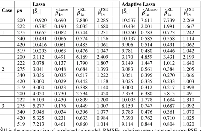
Result: We plot the mean RMSEs from 1000 iterations along pn in Figure 1. Some selected results are also reported in Table 1. To check the behavior of Lasso or adaptive Lasso for subset selection, we also report the average number of selected important covariates as in Table 1. It is not surprising to see that RE post the adaptive Lasso is comparable with the adaptive Lasso itself, while RE post the Lasso behaves much better than Lasso [13, 14]. We summarize the simulation results as follows:
• Figure 1(a')–(c') lists results when the adaptive Lasso is used to generate the submodel. (i) When pn is closer to n, both post selection RE and adaptive Lasso perform better than the post selection PSE and WR (RMSE > 1). (ii) When pn grows bigger, both RE and
adaptive Lasso become worse than the post selection WR (RMSE < 1). However, the post selection PSE still performs better than the post selection WR. Therefore, the post
selection PSE provides a protection of the adaptive Lasso in the case that the adaptive Lasso loses its efficiency.
• Figure 1(a)–(c) lists results when the Lasso is used to generate the submodel. The
advantage of the post selection PSE over the Lasso is more obvious than the earlier. This is because the adaptive Lasso tends to produce a more efficient estimator than the Lasso does.
• When pn grows, the post selection PSE is much more robust and at least as good as the WR estimator (RMSE is approaching to 1). When pn grows bigger, the improvement of the post selection PSE from adaptive Lasso or Lasso becomes more obvious. See Table 1.
• In Case 3, the post selection PSE may lose its superiority to the post selection RE and adaptive Lasso, especially when pn grows quickly with n. One explanation is that the selected model size varies dramatically because the number of weak coefficients grows. However, if we still follow the model parsimony spirit and decide to use an aggressive tuning parameter to obtain a relatively consistent submodel size , the superiority of post selection PSEs follows the same pattern as in Cases 1 and 2.
Table 1. Simulated RMSEs from simulation examples in Case 1–3.
Lasso Adaptive Lasso
Case pn 200 10.920 0.690 7.880 2.285 10.537 7.611 7.739 2.269 222 10.785 0.190 2.035 1.680 10.434 2.001 1.991 1.667 1 275 10.655 0.082 0.744 1.231 10.250 0.783 0.773 1.242 340 10.491 0.066 0.574 1.126 10.137 0.585 0.558 1.114 420 10.416 0.061 0.485 1.061 9.906 0.514 0.491 1.062 519 10.293 0.063 0.476 1.047 9.781 0.480 0.446 1.042 200 3.112 0.491 6.169 2.409 3.170 4.859 3.431 2.199 222 3.078 0.137 1.790 1.807 3.149 1.447 1.012 1.640 2 275 3.041 0.048 0.684 1.393 3.083 0.561 0.384 1.205 340 3.036 0.035 0.517 1.222 3.051 0.395 0.270 1.066 420 3.000 0.029 0.442 1.138 3.025 0.335 0.233 1.003 519 3.000 0.023 0.388 1.140 3.000 0.312 0.217 0.998 200 4.020 0.730 2.594 1.420 7.379 6.380 5.815 1.491 222 6.109 0.430 0.809 1.200 10.005 1.778 1.684 1.310 3 275 5.277 0.176 0.449 1.007 8.159 0.747 0.687 1.092 340 3.046 0.034 0.396 1.077 3.783 0.476 0.361 1.070 420 5.325 0.231 0.633 0.984 7.390 0.762 0.710 1.025 519 7.213 0.461 0.860 1.014 9.114 0.844 0.804 1.020
|Ŝ1| is the average size of produced submodel; RMSEs, relative mean squared errors;PSE, post selection shrinkage estimator; RE, restricted estimator.
Figure 1. Relative mean squared errors (RMSEs) of post selection relative mean squared errora (PSEs) compared with one from Lasso or adaptive Lasso (ALasso) from simulation examples in Cases 1–3. The top (a or a'), middle (b or b'), and bottom (c or c') panels are for Cases 1, 2, and
3, respectively. The left (a–c) and right panels (a'–c') are comparisons when the candidate submodels are chosen from the Lasso and adaptive Lasso methods, respectively.
6 Real-data example
In this section, we apply the proposed post selection shrinkage strategy to the growth data for the years 1960–1985 [30]. Table 2 lists the detailed descriptions of the dependent variable and 45 covariates related to education and its interaction with lgdp60i, market efficiency, political stability, market openness, and demographic characteristics.
Table 2. List of variable.
Variable Description
Dependent variable
gr Annualized GDP growth rate in the period of 1960–85 Threshold variables
gdp60 Real GDP per capita in 1960 (1985 price)
Covariates
lgdp60 log GDP per capita in 1960 (1985 price)
lsk Log(Investment/Output) annualized over 1960–85; a proxy for the log physical savings rate
lgrpop Log population growth rate annualized over 1960–1985
pyrm60 Log average years of primary schooling in the male population in 1960 pyrf60 Log average years of primary schooling in the female population in 1960 syrm60 Log average years of secondary schooling in the male population in 1960 syrf60 Log average years of secondary schooling in the female population in 1960 hyrm60 Log average years of higher schooling in the male population in 1960 hyrf60 Log average years of higher schooling in the female population in 1960 nom60 Percentage of no schooling in the male population in 1960
nof60 Percentage of no schooling in the female population in 1960
prim60 Percentage of primary schooling attained in the male population in 1960 prif60 Percentage of primary schooling attained in the female population in 1960 pricm60 Percentage of primary schooling complete in the male population in 1960 pricf60 Percentage of primary schooling complete in the female population in 1960 secm60 Percentage of secondary schooling attained in the male population in 1960 secf60 Percentage of secondary schooling attained in the female population in 1960 seccm60 Percentage of secondary schooling complete in the male population in 1960 seccf60 Percentage of secondary schooling complete in the female population in 1960 llife Log of life expectancy at age 0 averaged over 1960–1985
lfert Log of fertility rate (children per woman) averaged over 1960–1985 edu/gdp Government expenditure on eduction per GDP averaged over 1960–1985 gcon/gdp Government consumption expenditure net of defence and education
per GDP averaged over 1960–85
revol The number of revolutions per year over 1960–84
wardum Dummy for countries that participated in at least one external war over 1960– 84
wartime The fraction of time over 1960–1985 involved in external war lbmp Log(1+black market premium averaged over 1960–85) tot The term of trade shock
lgdp60 ‘educ’ Product of two covariates (interaction of lgdp60 and education variables from pyrm60 to seccf60); total 16 variables
The growth regression model has been applied to test the negative relationship between the long-run growth rate and the initial GDP given other covariates. See [31] and [32] for literature reviews. Very recently, [33] took into account the possible discrepancy among the
aforementioned negative relationship using a growth regression model with threshold. In particular, they consider a threshold variable in the following regression model,
(6.1)
where gri is the annualized GDP growth rate of country i from 1960 to 1985, lgdp60i is the log GDP in 1960, zi includes all 45 covariates listed in Table 2, and Qi is a threshold variable, where we use the initial GDP in 1960. Because the estimation of the threshold parameter τ is not our target, we consider five different τ's in our analysis: 1655, 2073, 2898, 3268, and 6030. Among them, τ = 2898 is a threshold value suggested by [33], and the other four threshold values are kth percentiles for k = 60,70,80,90, respectively. After removing all missing data, each setting includes n = 82 observations and p = 90 covariates besides two intercepts.
Before applying the post selection shrinkage strategy, we first obtain candidate subsets from two variable selection techniques: Lasso and adaptive Lasso, respectively. All tuning parameters are selected from fivefold cross validation. In Table 3, we list the numbers of selected important variables, , and also the sizes of candidate submodels, under five different τ's. In Table 4, we list the frequency of each variable being selected among all five settings. We observe that Lasso and adaptive Lasso variable selection results in Table IV are quite close for this data set. However, the selected candidate subset model can be quite different among all five different τ's.
Table 3. Sizes of selected submodel.
τ 6030 3268 2898 2073 1655
Lasso 15 18 18 19 11
adaptive Lasso 19 13 20 19 11
Table 4. Frequency of selected variables (based upon either βj ≠ 0 or δj ≠ 0) among All 5 τ's.
Variable Lasso ALasso
#(βj ≠ 0) #(δj ≠ 0) #(βj ≠ 0) #(δj ≠ 0)
lgdp60 5 0 5 0
nom60 0 1 0 1 prim60 3 0 3 0 pricm60 3 3 3 3 seccm60 0 5 0 5 seccf60 1 0 1 0 llife 5 0 5 0 lfert 5 0 5 0 edugdp 3 0 4 0 gcongdp 5 0 5 0 revol 2 0 3 0 wardum 2 3 2 3 wartime 4 4 3 3 lbmp 5 0 5 0 tot 0 5 0 5 lgdpsyrm60 2 0 2 0 lgdphyrm60 3 0 1 0 lgdphyrf60 0 1 1 0 lgdpnof60 0 3 0 3 lgdpprim60 2 0 2 1 lgdpprif60 0 1 0 2 lgdpseccf60 1 0 0 0
After the variable selection, post selection PSE is applied based upon the selected candidate subsets in all settings. Tables 5 and 6 give the estimation results for τ = 2898 and τ = 1655, where both candidate subsets are selected by the adaptive Lasso. We omit results under other settings to save the space.
Table 5. Estimation results under τ = 2898 (Candidate submodel from ALasso). Variable lgdp60 − 9.253 × 10 − 3 — − 1.287 × 10 − 2 — lsk 6.121 × 10 − 4 — 3.942 × 10 − 4 — nom60 — 1.400 × 10 − 2 — 3.481 × 10 − 2 prim60 − 4.579 × 10 − 2 — − 7.472 × 10 − 2 — pricm60 1.934 × 10 − 2 1.974 × 10 − 3 4.129 × 10 − 2 7.058 × 10 − 3 seccm60 — 4.903 × 10 − 4 — 4.324 × 10 − 4 llife 1.200 × 10 − 3 — 2.212 × 10 − 3 — lfert − 1.659 × 10 − 3 — − 1.507 × 10 − 3 — edugdp 2.228 × 10 − 5 — 2.309 × 10 − 5 — gcongdp − 2.351 × 10 − 4 — − 2.610 × 10 − 4 — revol − 1.020 × 10 − 6 — − 1.158 × 10 − 4 — wardum — − 1.417 × 10 − 4 — − 3.336 × 10 − 4 wartime − 1.655 × 10 − 4 — − 5.081 × 10 − 5 — lbmp − 1.580 × 10 − 3 — − 1.595 × 10 − 3 — tot — 5.202 × 10 − 6 — 6.318 × 10 − 6 lgdphyrm60 1.122 × 10 − 2 — 4.291 × 10 − 2 —
lgdphyrf60 − 7.585 × 10 − 3 — − 4.143 × 10 − 2 —
lgdpnof60 — 6.392 × 10 − 2 — 0.189
lgdpprif60 — − 3.130 × 10 − 2 — − 0.127
Table 6. Estimation results under τ = 1655 (Candidate submodel from ALasso). Variable lgdp60 − 2.841 × 10 − 3 — − 1.306 × 10 − 2 — lsk 1.319 × 10 − 3 — 1.284 × 10 − 3 — seccm60 — 3.652 × 10 − 4 — 5.873 × 10 − 4 llife 3.532 × 10 − 4 — 1.633 × 10 − 3 — lfert − 2.552 × 10 − 4 — − 2.250 × 10 − 3 — gcongdp − 1.554 × 10 − 4 — − 3.033 × 10 − 4 — revol − 3.715 × 10 − 5 — − 9.248 × 10 − 4 — wartime − 4.965 × 10 − 5 − 1.120 × 10 − 5 2.731 × 10 − 4 − 3.958 × 10 − 5 lbmp − 1.428 × 10 − 3 — − 5.887 × 10 − 4 — tot — 5.175 × 10 − 7 — 8.476 × 10 − 6
Becuase we do not know what the true model is in the real-data analysis, we first evaluate the prediction improvement from variable selection estimates to post selection PSEs by computing the relative residual sum of squares (RRSS) of the estimator over the WR estimator as follows:
(6.2)
where is the index of the submodel chosen by corresponding variable selection methods, and can be (adaptive) Lasso and the corresponding generated post selection SEs and post selection PSEs. Similar to the simulation studies, RRSS > 1 indicates the superiority of
over . The results on RRSS for different τ's are reported in Figure 2, where the left and right panels are based upon Lasso and adaptive Lasso submodels, respectively. Those RRSS values of post selection REs give the highest value in both cases. This is not surprising because we assume the selected submodel is the right one and does not account for any bias. In both cases, the post selection PSEs dominate the corresponding variable selection estimation in terms of the RRSS regardless of whether Lasso or adaptive Lasso is used for generating the candidate submodel. This is because shrinkage estimation provides a better trade-off between bias and variance when selected submodels underfit the true model.
Figure 2. Relative residual sum of squares (RRSS) from (6.2) from post selection post selection shrinkage estimator (PSE) and the Lasso-type estimators: Lasso (left panel) or adaptive Lasso (ALasso) (right panel). The curve is plotted based upon a decreasing order of RRSS for better visibility, with corresponding values of τ plotted in x-axis.
In addition, we also obtain prediction errors using cross validation following 500 random partitions of the data set. In each partition, the training set consists of 2/3 observations (size 55), and the test set consists of the remaining 1/3 observations (size 28). Corresponding results for τ = 2898 and 1655 are reported in Figure 3, where the post selection PSEs are compared with the adaptive Lasso. The comparisons between the post selection PSEs and (adaptive) Lasso for other τ's follow the similar pattern and thus are omitted. It is observed that post selection PSEs produce much smaller prediction errors than the Lasso-type estimation.
Figure 3. Prediction errors from post selection post selection shrinkage estimator (PSE), restricted estimator (RE), and adaptive Lasso (ALasso). Left: τ = 2898; Right: τ = 1655. All prediction errors are computed using cross validation following 500 random partitions of the data set. In each partition, the training set consists of 2/3 observations, and the test set consists of the remaining 1/3 observations.
7 Conclusion and discussions
In this paper, we generalize the shrinkage estimation to a high-dimensional sparse regression model. We propose a post selection shrinkage estimation strategy by shrinking a WR estimator in the direction of a candidate submodel obtained by existing PLSs variable selection methods. When pn grows with n quickly, it is reasonable to assume that the model sparsity exists in the sense that most covariates do not contribute. However, at the same time, some covariates may still make some small but jointly non-trivial contribution to the response. Existing penalized regularization approaches usually lead to a sparse model but tend to miss the possible small contributions from some covariates, resulting in excessive prediction errors or inefficient estimation. Our proposed post selection shrinkage strategy, taking into account possible contributions of covariates with weak and/or moderate signals, has dominant prediction performances over candidate submodel estimates generated from Lasso-type methods.
Before obtaining a shrinkage estimator, one key step is to generate a full estimation
of βn when p ≫ n. We suggest a post selection WR estimator which is able to separate small coefficients from zero coefficients. The advantages of proposed post selection PSE are studied both theoretically and numerically. In theory, we established the asymptotic normality of the post selection WR estimator when pn grows with n at an almost exponential rate such that
log(pn) = O(nν) for some 0 < ν < 1. Those novel asymptotic properties are used for investigating the asymptotic efficiency of the proposed post selection PSE analytically. In numerical studies, we chose tuning parameters c1 and c2 from cross validation but cannot guarantee their optimality for post selection PSE. The choice of tuning parameters is an important but challenging issue in high-dimensional data analysis that could potentially create very important future work.
Although the proposed post selection PSE was presented based on a WR method, other methods can also be used to generate the shrinkage estimator.
Finally, we acknowledge the importance of Lasso-type variable selection methods, but at the same time, and do not depend completely on them, especially when many weak coefficients jointly affect the response variable. The Lasso is the start but not the end. We could potentially still make some significant prediction improvements. We hope this work will shed some more light on the investigation of the post variable selection shrinkage analysis in high-dimensional data analysis.
Appendix
All technical proofs are given in this section.
Proof of Theorem 1. After solving (3.1), we obtain
(A1) and
(A2)
where and .
We only need to prove the result under the condition , and then all matrices, vectors indexed by can be replaced by S1 or 1 without causing of any confusion. For
example, under the condition.
First, we check the bias of . Because M1 is an idempotent matrix, M1X1n = 0. Denote qn = p2n + p3n. Then,
Let Q be a qn × qn orthogonal matrix such that
where . Then, we have
(A3)
Suppose that Q = (Q1,Q2) and Q1 is a qn × kn matrix. Notice that . Then, , Q1′Q2 = 0, and Q2Q2′ is a projection matrix. Let . Then,
(A4) Replace in (A3) by , we have
Thus,
For every , and thus,
The rest of the proof just mimics the proof of Theorem 2 in [28]. We will provide some outlines of the proof. If we let and log(pn) = O(nν) in (B3), then
where the last ‘≤’ is from (3.5) and c1 is defined there. From the normal assumption of ϵi and the solution in linear expression in (A2), we know is normally distributed and
where ‘A≼B’ means B − A is a non-negative definite matrix. Thus, for
any . Notice that . We
have
where Φ is the cumulative distribution function of a standard normal random variable, c0 > 0 is a constant, ‘≤’ is the tail probability of a normal random variable. Thus,
When n is large enough, there exists for some t > 0. Thus,
Similarly, we have
Because of the continuity of and , we have
Proof of Corollary 1. Because , a weighted ridge estimator aims to find some weak signals from . Because , the smallest positive eigenvalues of must be larger than λ1n, and . Thus, we can borrow the proof of Theorem 1 here, by treating and as the new S1 and S2.
Proof of Theorem 2. Similar to the proof in Theorem 1, we assume . Then, the penalized quadratic loss function in (3.1) becomes
From the notation . If we write , then
Replacing yi by , we have
Notice that . Thus,
(H5)
Under conditions (B1–B3), with probability 1, from Theorem 1. Therefore, the third term in (H5) is zero. By abusing the notation, if we rewrite dn = (d1n′,d2n′)′, then
where the first ‘≤’ is from (B4), the first ‘=’ is from (A2) and (B1), the second ‘≤’ is from the Cauchy–Schwarz inequality, the third ‘≤’ is from (A2). The last ‘=’ holds because rn = o(n1/2 − τ) if we choose with an = c1n − α for α < 1/4 − τ/2 for 0 < τ < 1/2. Therefore,
(H6) Define 𝑈𝑖 = 𝑛−1∕2𝑠
𝑛−1𝑑𝑛′𝛴𝑛−1𝑧𝑖̇, 1 ≤i≤n. From (B1), we know that ∑𝑛𝑖=1𝑢𝑖𝜀𝑖 is normal with variance,
Proof of Theorem 3. First, (4.9a) holds because we have
where Z ∼ N(0,1). We now verify (4.9b). Let 𝑦̃ = 𝑦 − 𝑋2𝑛𝛽̂2𝑛𝑤𝑅− 𝑋3𝑛𝛽̂3𝑛 Then,
(H7) From the definition,
From (4.9a), we know 𝐼1 = lim 𝑛 → ∞ ∈ {𝑛1∕2𝑠
1𝑛−1𝑑1′𝑛(𝛽̂1𝑛𝑤𝑅− 𝛽1∗)} 2
. From (H7),
where 𝑑2𝑛= 𝛴𝑛21𝛴𝑛11−1𝑑
1𝑛 and 𝑆2𝑛2 = 𝑑2𝑛′ 𝛴𝑛22.1−1 𝑑2𝑛. From Ouellette (1981) Equation (1.12), we obtain
Therefore,
Because 𝑠2𝑛2 ∕ 𝑠
1𝑛2 → 1 − 𝑐,
where 𝑥𝑣2(𝑡) is a χ2 distribution with degrees of freedom ν and noncentral parameter t. Here, Δd1n is given in (4.8). From the Cauchy–Schwarz inequality,
Furthermore,
Thus, 𝑅(𝑑1𝑛′ 𝛽̂1𝑅𝐸𝑛 ) = 𝐼1+ 𝐼2+ 𝐼3 = 1 − (1 − 𝛥𝑑1𝑛)(1 − 𝐶). Thus, (4.9b) holds. We now investigate (4.9c). First from the definition,
Again, J1= lim 𝑛 → ∞{𝑛1∕2𝑠
1𝑛−1𝑑1′𝑛(𝛽̂1𝑛𝑤𝑅− 𝛽1∗)} 2
Then, we have
From Theorem 1, 𝑠̂2 = 𝑝2𝑛+ 𝑜𝑝(1) and
We now define ,
and η(x) = ((p2n − 2)/(x′Wx))b′x, where 𝑤 = (
0 0
0 𝛴𝑛22.1) Then, from the asymptotic normality,
where and z satisfy that
and
So we have
where
Notice that 𝑎′𝛴
𝑛−1𝑏 = 𝑑2𝑛′ 𝛴𝑛21.1−1 𝑑2𝑛= 𝑠2𝑛2 and 𝑊𝛴𝑛−1𝑎𝑏′= 𝑏𝑏′ Therefore,
Thus,
Proof of Corollary 3. We first verify (i).
Define and . From the
Cramér–Wold device, we have
where Δn = δ′Σn22.1δ and ‘Tr(B)’ is the trace of matrix B. Here, the second ‘=’ is from Theorem 8 in Chapter 2 in [29]. Notice that Tr(B) = 1. Using the relationship between the chi-square distribution and Poisson distribution,
where κ is a Poisson distribution with mean Δn/2 and Eκ means the expectation is taken for the Poisson random variable κ. Because P(k≥ 1) when p2n ∞. With almost probability 1, we have
If ∥δ∥2≤1, then . Then, E[g1(z2
+ 𝛿]. Furthermore, when x′Σn22.1x≤p2n − 2, we have
In fact, the inequalities in (i) also hold even though ∥δ∥2 > 1. For example, suppose Δn = ιp 2n for some constant ι > 0. Then, . Therefore, if ∥δ∥2≤1 + ι, with probability 1, we have
Thus, (ii) holds.
We now verify (iii). If δ = 0, then Δd1n = 0. Thus, .
We now compare with .
Denote . If δ = 0, then we have
From Theorem 2.1.8 in [29] and moment of inverse chi-squares distribution, we have
and
Thus, if p2n = p2 is fixed, E[g1(z2)] = (1 − c)(1 − 2/p2) < 1 − c. Therefore,
References
1 Tibshirani R. Regression shrinkage and selection via the Lasso. Journal of the Royal Statistical Society, Series B 1996; 58:267–288.
2 Leng C, Lin Y, Wahba G. A note on the Lasso and related procedures in model selection. Statistica Sinica 2006; 16:1273–1284.
3 Fan J, Li R. Variable selection via nonconcave penalized likelihood and its oracle properties. Journal of the American Statistical Association 2001; 96:1348–1360.
4 Fan J, Lv J. Nonconcave penalized likelihood with np-dimensionality. IEEE Transactions on Information Theory 2011; 57(8):5467–5484.
5 Zou H. The adaptive Lasso and its oracle properties. Journal of the American Statistical Association 2006; 101:1418–1429.
6 Zhang CH. Nearly unbiased variable selection under minimax concave penalty. The Annals of Statistics 2010; 38(2):894–942.
7 Fan J, Lv J. A selective overview of variable selection in high dimensional feature space. Statistica Sinica 2010; 20(1):101.
8 Zhang CH, Zhang SS. Confidence intervals for low dimensional parameters in high
dimensional linear models. Journal of the Royal Statistical Society: Series B 2014; 76(1):217– 242.
9 Zhao P, Yu B. On model selection consistency of LASSO. Journal of Machine Learning Research 2006; 7:2541–2563.
10 Huang J, Ma SG, Zhang CH. Adaptive Lasso for sparse high-dimensional regression models. Statistica Sinica 2008; 18:1603–1618.
11 Bickel P, Ritov Y, Tsybakov A. Simultaneous analysis of Lasso and dantzig selector. Annals of Statistics 2009; 37:1705–1732.
12 Hansen BE. The risk of James-Stein and Lasso
shrinkage, 2013. http://www.ssc.wisc.edu/bhansen/papers/lasso.pdf [accessed 20 December 2015] .
13 Belloni A, Chernozhukov V. Least squares after model selection in high-dimensional sparse models. Bernoulli 2009; 19:521–547.
14 Liu H, Yu B. Asymptotic properties of Lasso+mLS and Lasso+Ridge in sparse high-dimensional linear regression. Electronic Journal of Statistics 2013; 7:3124–3169.
15 Stein C. 1956. Efficient nonparametric testing and estimation. In Proceedings of the Third Berkeley Symposium on Mathematical Statistics and Probability, 1954–1955, vol. I. University of California Press: Berkeley and Los Angeles; 187–195.
16 James W, Stein C. Estimation with quadratic loss. Proceedings of the Fourth Berkeley Symposium on Mathematical Statistics and Probability 1961; 1:361–379.
17 Ahmed SE. Penalty, Shrinkage and Pretest Strategies: Variable Selection and Estimation. Springer: New York, 2014.
18 Ahmed SE, Fallahpour S. Shrinkage estimation strategy in quasi-likelihood models. Statistics & Probability Letters 2012; 82:2170?2179.
19 Ahmed SE, Hossain S, Doksum KA. Lasso and shrinkage estimation in Weibull censored regression models. Journal of Statistical Inference and Planning 2012; 12:1273–1284. 20 Ahmed SE, Doksum KA, Hossain S, You J. Shrinkage, pretest and absolute penalty estimators in partially linear models. Australian & New Zealand Journal of
Statistics 2007; 49:435–454.
21 Marsaglia G, Styan GPH. Equalities and inequalities for ranks of matrices. Linear and Multilinear Algebra 1974; 2:269–292.
22 Frank IE, Friedman JH. A statistical view of some chemometrics regression tools (with discussion). Technometrics 1993; 35:109–148.
23 Zhang CH, Huang J. The sparsity and bias of the LASSO selection in high-dimensional linear regression. The Annals of Statistics2008; 36:1567–1594.
24 Chen SS, Donoho DL, Saunders MA. Atomic decomposition by basis pursuit. SIAM Journal on Scientific Computing 1998; 20(1):3361.
25 Wainwright MJ. Sharp thresholds for high-dimensional and noisy sparsity recovery using ℓ 1-constrained quadratic programming (Lasso). IEEE Transactions on Information
Theory 2009; 55(5):2183–2202.
26 Zheng Z, Fan Y, Lv J. High dimensional threshold regression and shrinkage effect. Journal of the Royal Statistical Society: Series B2014; 76:627–649.
27 Weng H, Feng Y, Qiao X. Regularization after retention in ultrahigh dimensional linear regression models, 2013. arXiv preprint arXiv:1311.5625.
28 Shao J, Deng X. Estimation in high-dimensional linear models with deterministic design matrices. Annals of Statistics 2012; 40:812–831.
29 Saleh A. KME. Theory of Preliminary Test and Stein-Type Estimation with Applications. Wiley: New York, 2006.
30 Barro R, Lee J. Data set for a panel of 139
countries, 1994. http://admin.nber.org/pub/barro.lee/ [accessed 20 December 2015]. 31 Barro R, Sala-i Martin X. Economic Growth. McGraw-Hill: New York, 1995.
32 Durlauf S, Johnson PA, Temple JRW. Growth econometrics. Handbook of Economic Growth 2005; 1:555–677.
33 Lee S, Seo MH, Y S. The LASSO for high-dimensional regression with a possible change-poin. Journal of the Royal Statistical Society: Series B 2016; 78:193–210.